Communication

A New Remote Sensing Method to Estimate River to Ocean DOC Flux in Peatland Dominated Sarawak Coastal Regions, Borneo

1
Faculty of Engineering, Computing and Science, Swinburne University of Technology, Kuching 93350, Sarawak, Malaysia
2
CSIRO Oceans and Atmosphere, Canberra ACT 2601, Australia
3
Faculty of Resource Science & Technology, University Malaysia Sarawak, Kota Samarahan 94300, Sarawak, Malaysia
4
Asian School of the Environment, Nanyang Technological University, Singapore 639798, Singapore
5
Institute of Environmental Physics, University of Bremen, Otto-Hahn-Allee 1, 28359 Bremen, Germany
6
Leibniz Center for Tropical Marine Research, Fahrenheitstr. 6, 28359 Bremen, Germany
7
Institute of Geology, University of Hamburg, 20146 Hamburg, Germany
*
Author to whom correspondence should be addressed.
Remote Sens. 2020, 12(20), 3380; https://doi.org/10.3390/rs12203380
Submission received: 30 July 2020 / Revised: 7 September 2020 / Accepted: 10 September 2020 / Published: 16 October 2020
(This article belongs to the Special Issue Remote Sensing of Carbon Cycle Science)

Abstract

:
We present a new remote sensing based method to estimate dissolved organic carbon (DOC) flux discharged from rivers into coastal waters off the Sarawak region in Borneo. This method comprises three steps. In the first step, we developed an algorithm for estimating DOC concentrations using the ratio of Landsat-8 Red to Green bands B4/B3 (DOC (μM C) = 89.86 · e 0.27 · ( B 4 / B 3 ) ), which showed good correlation (R = 0.88) and low mean relative error (+5.71%) between measured and predicted DOC. In the second step, we used TRMM Multisatellite Precipitation Analysis (TMPA) precipitation data to estimate river discharge for the river basins. In the final step, DOC flux for each river catchment was then estimated by combining Landsat-8 derived DOC concentrations and TMPA derived river discharge. The analysis of remote sensing derived DOC flux (April 2013 to December 2018) shows that Sarawak coastal waters off the Rajang river basin, received the highest DOC flux (72% of total) with an average of 168 Gg C per year in our study area, has seasonal variability. The whole of Sarawak represents about 0.1% of the global annual riverine and estuarine DOC flux. The results presented in this study demonstrate the ability to estimate DOC flux using satellite remotely sensed observations.

Graphical Abstract

1. Introduction

Dissolved organic carbon (DOC) is an important component in the global carbon cycle. This is particularly true for the ocean, where DOC represents about 97% of the organic carbon pool [1]. One of the main inputs of DOC to the ocean is from rivers, with approximately 62% of this export occurring in tropical regions [2]. The discharge into the South China Sea (covering 1% of the world’s ocean) accounts for almost 10% of global riverine DOC fluxes [3]. The high contribution is due to extensive peat deposits along the coasts of Borneo and Sumatra [4,5]. These peatlands are drained by rivers that carry up to 52 mg L 1 organic carbon, mostly in form of DOC [6]. The transfer of carbon from terrestrial pools to aquatic bodies affects the concentrations and dynamics of organic carbon transformations, and lastly the marine ecosystems [7] and CO 2 outgassing at the coastal waters [5]. Despite the importance of robust riverine and estuarine DOC flux estimates, large uncertainties remain due to limitations in data and access to remote sites.
Traditional field-based methods to monitor DOC in aquatic systems are costly and labor-intensive. Remote sensing technologies are cost effective and they provide high frequency data across broad spatial scales for aquatic biogeochemical parameters [8]. Aquatic biogeochemical remote sensing is determined by the inherent optical properties of water [9]. Coloured dissolved organic matter (CDOM) is the optically-active component of DOC. Examples of recent remote sensing studies on CDOM are Cardille, et al. [10], Zhu, et al. [11], Cao & Miller, [12], Brezonik, et al. [13], Joshi & D’Sa, [14], Cao, et al. [15], Chen, et al. [16], Li, et al. [17], Xu, et al. [18], Cherukuru, et al. [19], Alcantara, et al. [20], Olmanson, et al. [21], Slonecker, et al. [22], Toming, et al. [23], Coelho, et al. [24], Griffin, et al. [25], and Herrault, et al. [26]. These studies covered a variety of water types (e.g., lake, river, and estuary) and remote sensing platforms (e.g., Landsat, MODIS, Sentinel, and MERIS). A strong linear correlation exists between CDOM and DOC in coastal waters dominated by terrestrial inpus of dissolved organic matter (DOM) [19,27]. Therefore, CDOM has often been used as an optical proxy to derive DOC concentration (see for example Cao et al. [15], Cherukuru et al. [19], Griffin et al. [25], and Herrault et al. [26]. The present study showcases the first application of Landsat-8 imagery to estimate DOC concentration in turbid waters for estuarine and coastal waters off Sarawak. This study uses Landsat-8 imagery, whereas, in other similar studies [19,28,29], MODIS and MERIS imagery were used. The advantage of Landsat-8 image is the higher spatial resolution (30 m) as compared to MODIS (250 m to 1000 m), although MODIS has a shorter revisit time (1 day) compared to Landsat-8 (16 days). Higher spatial resolution offers insights into processes at finer scales and, thus, enables a better understanding of the connection between inland, estuarine, and coastal aquatic ecosystems.
Besides DOC concentration, a second required parameter for DOC flux calculations is river discharge. River discharge is often calculated from precipitation data due to the lack of gauge stations [30,31,32]. The ability to capture spatial and temporal variability of precipitation data are, therefore, important towards understanding hydrological processes. However, accurate precipitation measurements over a large spatial scale are difficult. The direct observation of ground meteorological stations (gauged data) is more accurate, but limited by station network density, terrain, and other factors. A number of remotely sensed precipitation products with high spatial and temporal resolution have been developed to address this problem. One of the products, TRMM Multi-Satellite Precipitation Analysis (TMPA) precipitation product [33] has been widely used in various climatic and hydrological studies [34]. The TMPA is a joint mission between the National Aeronautics and Space Administration (NASA) and the Japan Aerospace Exploration Agency (JAXA) designed to monitor and study tropical rainfall. Examples of TMPA precipitation studies near our study area include Mahmud et al. [35] for Peninsula Malaysia, Tan & Duan [36] for Singapore, Takahashi et al. [37] for Borneo, Sun [38] for Sarawak, As-syakur et al. [39] for Indonesia, and Hidayat et al. [40] for Kalimantan. All of these studies have shown that simulated precipitation data from TMPA are highly accurate and reliable.
Combining Landsat-8-derived DOC concentrations with TMPA-derived river discharge has the potential to offer DOC flux estimates over large spatial-temporal scales. Thus, we aim to develop a new remote sensing method in order to estimate DOC flux from rivers and estuaries into coastal waters. This new method comprises three steps: (1) The first step involved development and validation of an algorithm to estimate DOC concentration from Landsat-8 optical data, (2) the second step involved the retrieval of precipitation data from TMPA and estimation of river discharge from river basins, and (3) the final step involves combining Landsat-8-derived DOC concentrations with TMPA-derived river discharge to estimate DOC flux Figure 1). We demonstrate our new method by estimating DOC flux into coastal waters from three estuaries (the Rajang, Sadong and Lundu) in Sarawak, Borneo, given the importance (and lack of data) of South East Asia for global DOC fluxes.

2. Materials and Methods
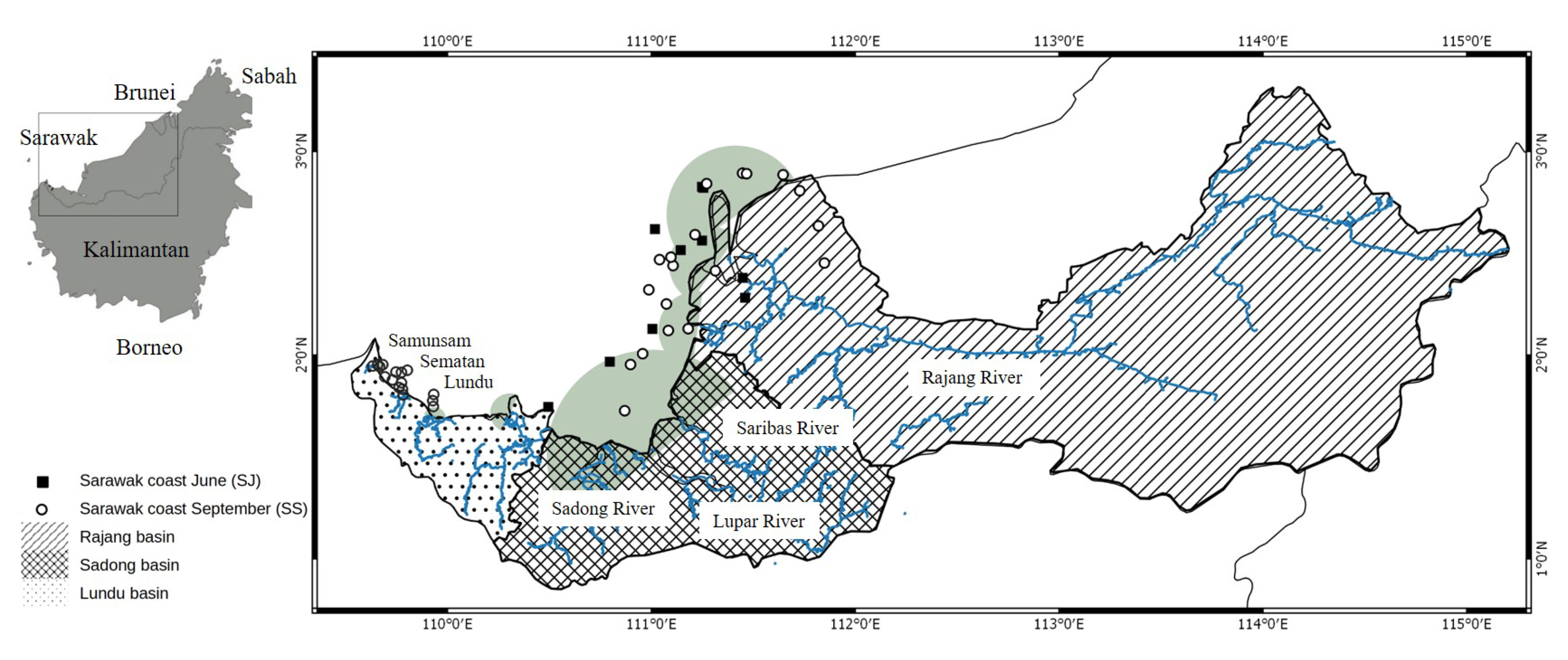
2.1. Study Area

Sarawak is in the northwest of the island of Borneo, and has a tropical rain forest climate. Our study focuses on river basins and coastal areas from the Rajang River (central Sarawak; longest river in Malaysia) to the Samunsam River in southwest Sarawak. Two field expeditions were undertaken in June 2017 (south-west monsoon, lower precipitation) and September 2017 (before the beginning of the north-east monsoon, end of drier season), covering 45 stations in total. The expedition in June 2017 focused on the coastal area from Kuching to the Rajang River. Ten coastal stations were covered during this expedition, including two stations in the Rajang River mouth. The expedition in September 2017 again covered the coastal area from Kuching to the Rajang River, but also the coastal area in southwest Sarawak (Samunsam, Sematan and Lundu). An overview of the sampling stations is shown in Figure 2. At each station, in-situ optical measurements were conducted and water samples collected for dissolved organic carbon (DOC) analyses (described in detail in Martin et al. [27].

2.2. Water Sampling

Analyses and discussion of DOC data are presented in [27]. In short, water samples were collected in the upper 1 m using a bucket or hand-held jug, and filtered through 0.2 μ m pore-size Anodisc filters (47 mm diameter). The samples (30 mL) were immediately acidified with 100 μ L of 50% H 2 S O 4 to pH <2.0, and stored in amber borosilicate EPA vials at 4 C until analysis. DOC was analyzed as non-purgeable organic carbon on a Shimadzu TOC-L system [27].
The datasets used in this study included measurements from two expeditions in June and September 2017, where a total of 45 stations were sampled. These two field expeditions represent environmental conditions associated with south-west monsoon (June 2017) and early stages of the north-east monsoon (September 2017). Table 1 shows the variability in physical and biogeochemical parameters in the surface waters during both expeditions. Because the sampling locations ranged from inside rivers to out in the open sea, a wide range was observed for parameters, such as depth, salinity, and total suspended solids (TSS) along the river, estuary, and open ocean continuum. DOC concentrations were the highest in the rivers (freshwater), reaching 1799 μ M in the Samunsam River, and gradually decreased to about 80 μ M in the open ocean (higher salinity).

2.3. In-Situ Optical Measurements

Water reflectance measurements were carried out using RAMSES (TriOS) sensors to measure downwelling irradiance ( E d ), sky irradiance ( E s k y ), and upwelling radiance ( L u ). E s k y and L u were used to calculate above-surface water-leaving radiance ( L w ). L w and average E d were used to compute remote sensing reflectance ( R r s = L w / E d ). Hyperspectral R r s data from RAMSES were used to simulate the R r s ( λ ) signals that would be recorded by the Landsat-8 sensor at each channels centered at wavelength λ . Weighted averages of each R r s spectrum were calculated by using the spectral band responses of OLI [41]. Landsat-8 OLI images provide four visible bands that can be used for coastal water remote sensing: B1 (433–453 nm), B2 (450–515 nm), B3 (525–600 nm), and B4 (630–680 nm).

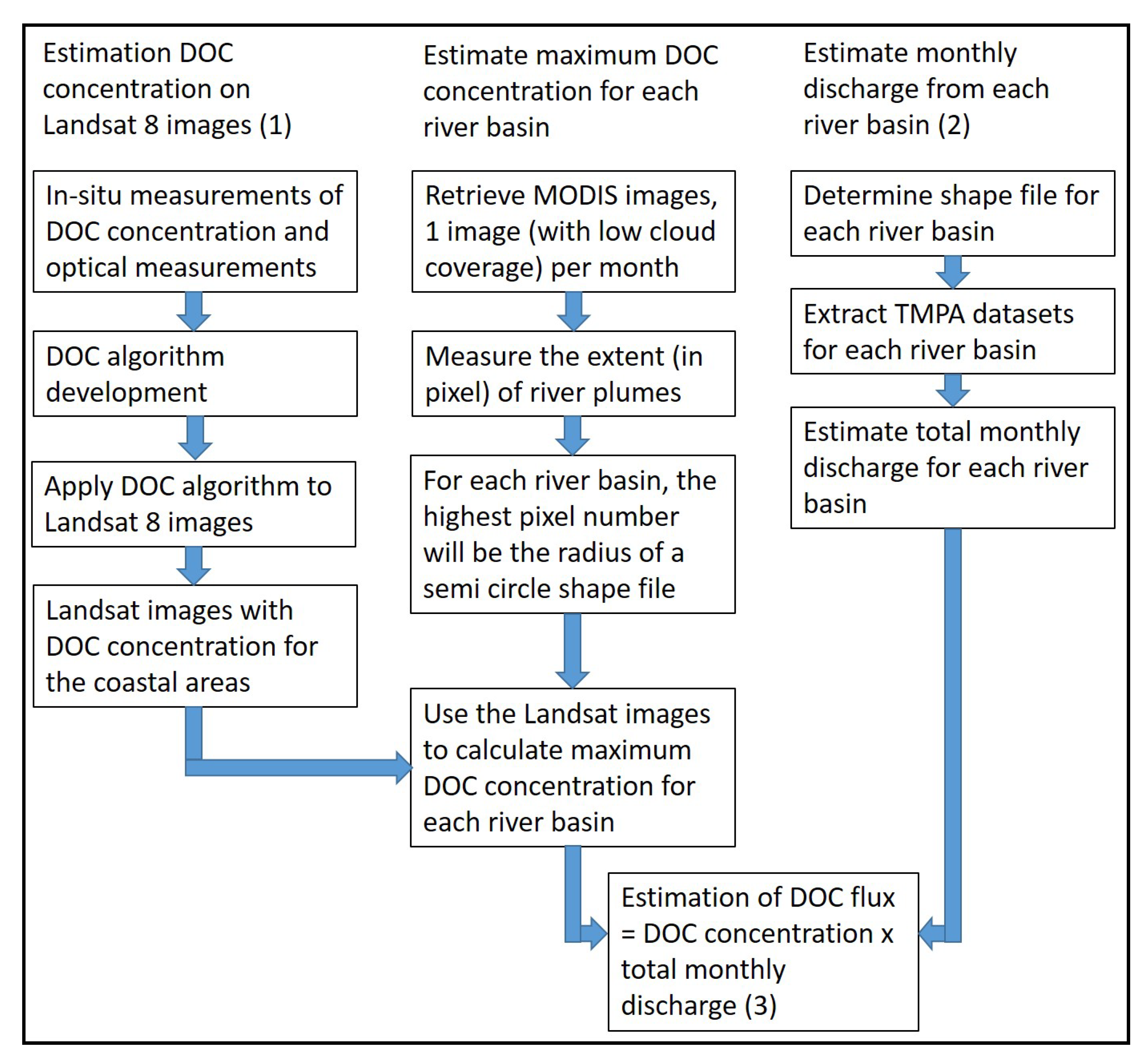
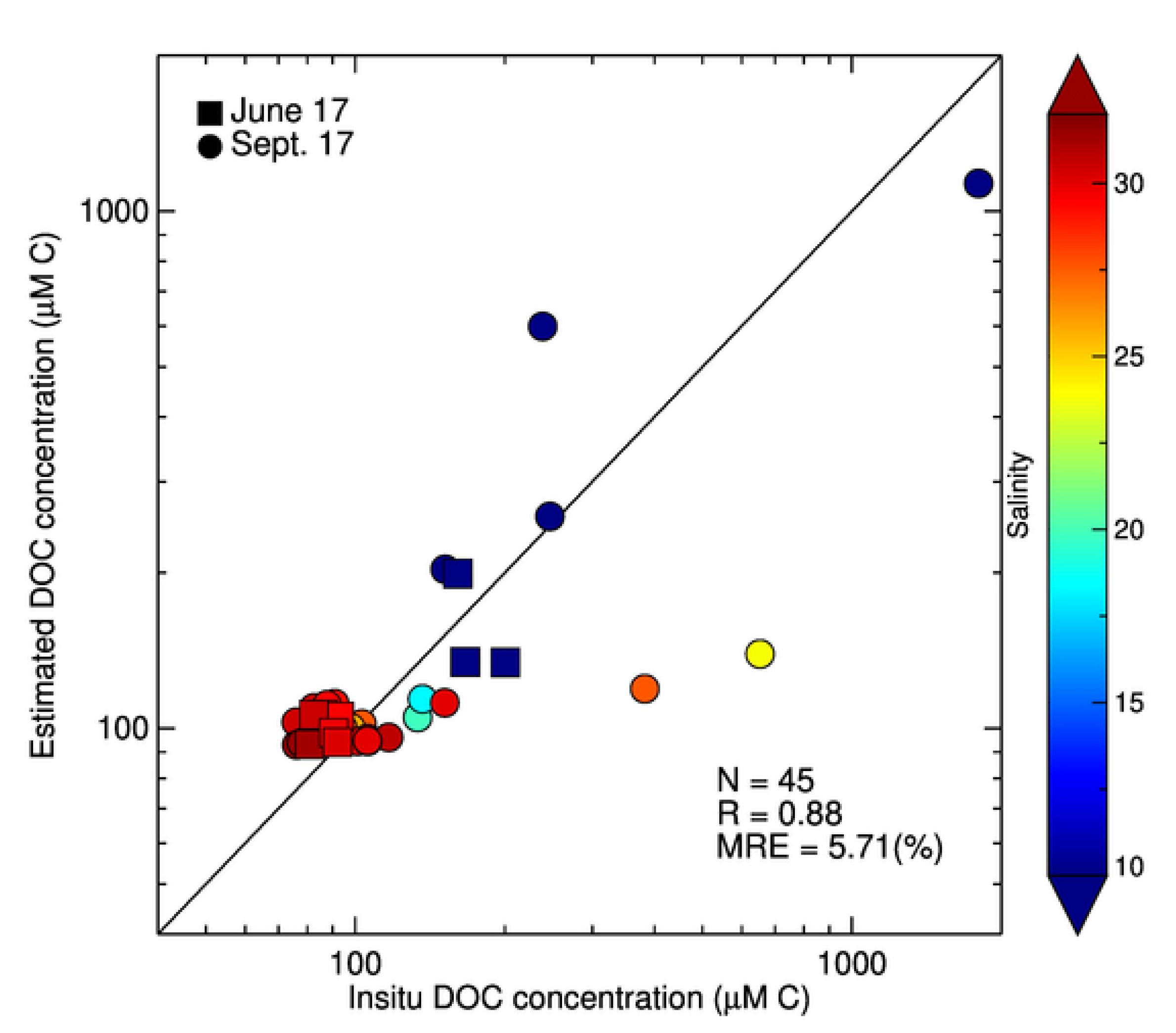
2.4. Algorithm Development, Validation, and Accuracy Assessment

DOC algorithm development for this study was based on CDOM studies using Landsat-8 images [16,20,22,42].To estimate the DOC concentration from Landsat-8 simulated R r s ( λ ) (equivalent to Landsat-8 bands), combinations of band ratios were adopted and regressed against in-situ DOC concentrations. Based on Chen et al. [16], we decided to focus on linear, power, exponential, and logarithmic models, images from Landsat-8 and band-ratio combinations of B2/B3, B3/B2, B2/B4, B4/B2, B3/B4, and B4/B3.
Three validation methods are performed in order to validate the algorithms. The first method is a simple grouping method, we group the 45 stations into three groups. In this method, one or two groups is/are used for algorithm calibration, the remaining group(s) used to test the algorithm. The second validation method is K-fold analysis from caret package in R [43]. In this analysis, the 45 stations are group into 9 groups. For each analysis, eight groups are used for calibration, the remaining group is used to test the algorithm. The third method is bootstrap method, We used resampling and bootstrap from R packages; rsample and nls [44]. For each model, we calculated accuracy for bootstrap-derived algorithms.
The accuracy of each algorithm was assessed based on correlation coefficient (R), coefficient of determination ( R 2 ), root mean squared error (RMSE) [45], and mean relative error, MRE (mean of 100*[model − measurement]/measurement).
Lastly, we used another set of independent data set of 63 stations (a table is available in the Supplementary Materials), to match Landsat-8 images with derived (from the selected exponential algorithm) DOC concentration.

2.5. Landsat-8 Image Acquisition and Estimation of DOC Concentration of Coastal Water

Level 1TP Landsat-8 OLI images were downloaded from the USGS website (http://glovis.usgs.gov/) and atmospheric correction was carried out using Acolite (Version 20190326; [46]. We used SNAP (Version 7.0; SNAP-ESA Sentinel Application Platform, http://step.esa.int) in order to apply the DOC algorithm to Landsat-8 images.

2.6. Estimate Maximum DOC Concentration for Each River Basin

Overall, we aimed to estimate DOC fluxes from the most likely riverine freshwater DOC concentration detected within the river plume areas. We developed an algorithm to estimate DOC concentration with in-situ remote sensing reflectance values in order to estimate DOC concentration within the river plume areas.
We used daily MODIS Aqua imagery for this purpose because of the high (daily) revisit frequency in order to quantify the spatial extent of river plumes beyond the center of each river mouth. One MODIS image (most cloud free) per month from year 2013 to 2018 was used for the measurements. We retrieved a total of 72 MODIS daily images with low cloud coverage. For each image, the measurements of the distance between the extent of river plumes and center of river mouths were recorded in the pixel unit. For each river basin, the river plume was approximated as a semi-circle centered on the river mouth, with a radius corresponding to the maximum river plume extent. Shape files of each river plume were produced using QGIS (Open Source Geospatial Foundation Project, http://qgis.osgeo.org). We combined several smaller river basins into the Sadong and Lundu basins because discharge from these smaller rivers mixes with the larger rivers. Hence, they were combined, and we partitioned the study area into three river basins. The biggest river basin is the Rajang basin (the longest river in Malaysia), followed by the Sadong basin and the Lundu basin. We then used the SNAP program to apply these shape files to the Landsat-8 images (with derived DOC concentration) to acquire the maximum DOC concentration for each river plume (Figure 2; land-masked pixels are ignored). In this study, we chose to use the maximum DOC concentration for the DOC flux estimation, as it represents the freshwater discharged DOC in a strong tidal mixing zone.

2.7. TMPA Data Acquisition and Estimation of Water Discharge

The precipitation over each river catchment was extracted from the TRMM Multisatellite Precipitation Analysis (TMPA). Satellite-derived precipitation products overcome the spatial coverage limitation of point-based ground observations [36]. Monthly precipitation data (TMPA version 3B43) were downloaded from the NASA Goddard Earth Sciences Data and Information Services Center (GES-DISC) website (GIOVANNI tool; https://giovanni.gsfc.nasa.gov/giovanni/). The precipitation data were multiplied by their respective basin size in order to estimate total precipitation for the basin. Total precipitation was then multiplied by surface runoff to estimate discharge for the whole basin. The estimated surface runoff for Sarawak is 60% of total precipitation, as detailed in [47].

2.8. DOC Flux Demonstration

We demonstrated the calculation of DOC flux from river basins into coastal waters using Landsat-8 images (to estimate riverine DOC concentrations) and TMPA data (to calculate monthly discharge for each basin). DOC flux was calculated as a product of both the maximum DOC concentration and water discharge, as summarized in Figure 1. We demonstrate the new method using data from the beginning of the Landsat-8 mission (April 2013) to the end of 2018.

3. Results

3.1. Determination of the Best DOC Algorithm for Landsat-8 in Sarawak Waters

In total, 24 models were tested (see Table 2). The results from the validation methods of grouping and K-fold analysis are similar, therefore only results from K-fold analysis are available in Table 2. The exponential model y = e 0.27 · ( B 4 / B 3 ) , where y is predicted DOC concentration and x is band ratio) with band ratio B4/B3 was selected based on its performance in validation analysis, R, R 2 , RMSE, and MRE. This exponential model performed better than the boot-strapping model with better MRE (+5.71%). Our in-situ DOC concentration was linearly related to the estimated DOC concentration (Figure 3).
Table 3 is the results for Landsat-8 derived DOC match up with independent data set from March 2017. 5 stations matched to a Landsat-8 image (2017-03-06-121058), and all of these stations are located in the cloud mask areas of the image. This is due to the long revisiting period of Landsat-8 (16 days) and high cloud coverage in the tropical climate. However, three stations are able to match to nearby pixels. MRE between the Landsat-8 image derived DOC concentration and measured DOC concentration range from −20.0% to −26.5%. This range is much higher than the MRE for the algorithm (+5.71%). Two factors contributed to this. The first factor is the satellite overpass time is at 10:00, whereas the sampling time for the five stations was conducted from 9:46 to 18:24. The second factor is the standard deviation for the DOC concentration measured at the stations is 29.7 μ M, this show high vulnerability of the DOC concentration in the water.

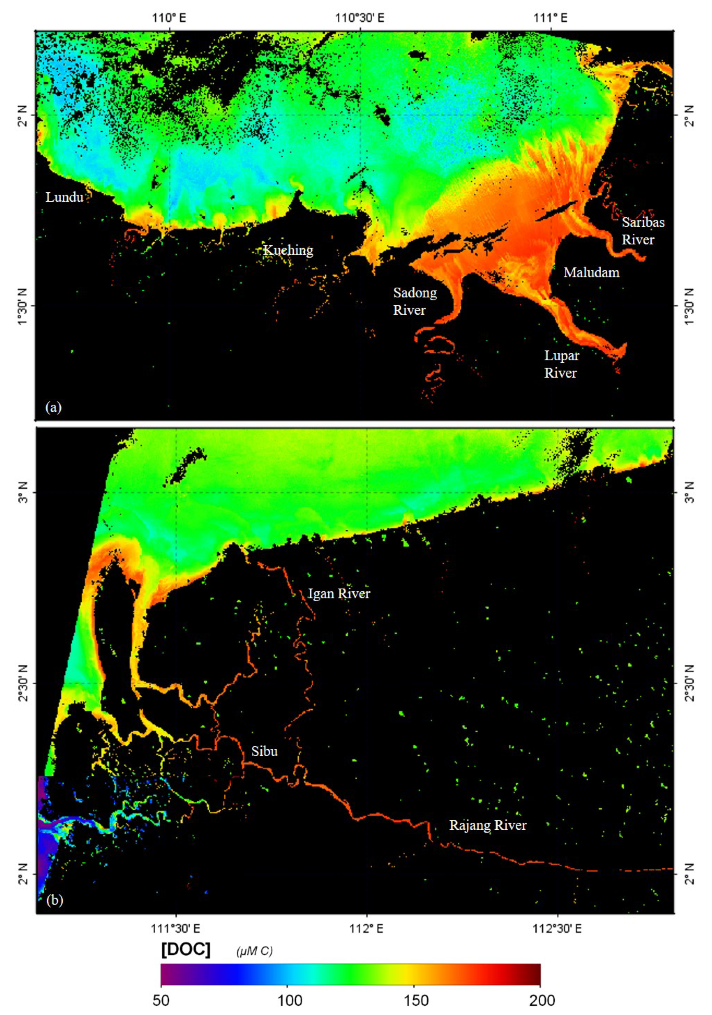
3.2. Applying the Algorithm to Landsat-8 Imagery

We applied the exponential model to Landsat-8 imagery from April 2013 to December 2018. We used four scenes of Landsat-8 images to capture the DOC concentrations for the three coastal areas (Rajang, Sadong and Lundu). Figure 4 shows a representative image with calculated DOC concentrations in the estuary and ocean. Estimated averaged maximum DOC concentration from April 2013 to December 2018 for the river plume areas are 121 (±2.6) μ M C (Lundu), 126 (±2.6) μ M C (Sadong), and 125 (±2.3) μ M C (Rajang). These DOC concentrations are within the range of DOC concentrations reported for lower estuary (salinity > 25 psu) Lupar River and Saribas River, 142 μ M C and 244 μ M C, respectively [48].

3.3. Calculation of Precipitation and Discharge from TMPA Dataset

The monthly precipitation (mm/month) TMPA version 3B43 was used to calculate average quarterly precipitation from April 2013 to December 2018. The TMPA product showed high correlation coefficient of 0.9 with the gauged data for Yangtze River delta [49]. For this study, the average estimated discharge from April 2013 to December 2018 is 3574 m 3 s 1 for Rajang, 1068.8 m 3 s 1 for Sadong, and 328 m 3 s 1 for Lundu. These values are in agreement with reported discharge data for Rajang, averaged 30 years of ground data of 3600 m 3 s 1 [50], TMPA data from 1998 to 2011 of 3450 m 3 s 1 [38] and ground data from 1992 to 2016 of 3322 m 3 s 1 [51].

4. Discussions

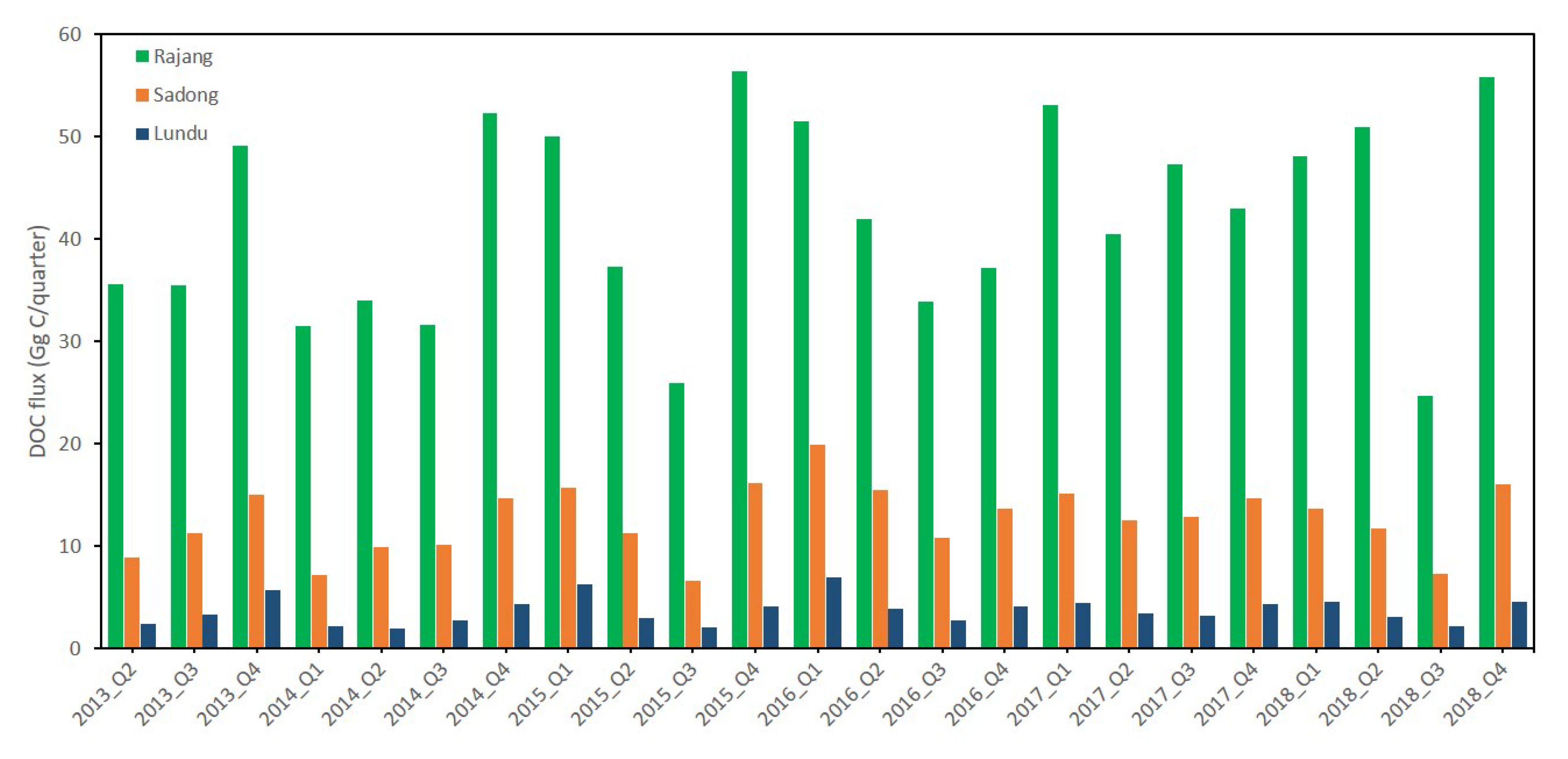
4.1. DOC Flux Variability in Sarawak Coastal Waters

Figure 5 summarises DOC fluxes (in Gg C per quarter) calculated using our newly developed method. Our study area experiences frequent cloud cover, which caused data gaps. Because of these gaps and the long revisit time of 16 days for Landsat-8, we summarise the data quarterly, and calculate average DOC fluxes for the three coastal areas from April 2013 to December 2018. The coastal waters off the Rajang basin receive the highest DOC flux (average 168 Gg C per year). This is due to the larger size of the Rajang basin compared to the Sadong and Lundu basins. The Rajang alone constitutes 72.5% of the total DOC flux from all three basins, revealing its importance for future management action. Time series analysis revealed strong seasonal variability, with the DOC fluxes highest in the monsoon season (from October to March, Q4 and Q1). The DOC flux is at times almost doubled in these quarters as compared to Q2 and Q3, highligthing the value of the high temporal resolution of our new method. Overall, the total annual DOC flux from the three basins (calculated using our new method) is, on average, 0.23 Tg C y r 1 . While this only represents about 0.1% of the global annual estuarine DOC flux [17], it is important to remember that the rivers studied cover only 0.05% [52] of the global river/estuarine area. Their contribution to global estuarine DOC fluxes is hence significant and our newly developed Landsat-8 remote sensing method allows for us to decipher their spatial and temporal patterns.

4.2. Uncertainties and Limitations

Uncertainty in DOC flux products generated in this study would be less than ±10%. Uncertainty in the final product will be contributions from the DOC algorithm fitting error (MRE +5.71%), which represents in-situ instrument and measurement errors. For the monthly discharge of each river basin, the uncertainties are from TMPA precipitation datasets and the estimation of river basin surface runoff. The nearest available comparison between TMPA datasets and rain gauge data is from a study conducted in Singapore [36]. Based on the study by Tan & Duan, [36], the TMPA dataset had underestimated the precipitation with MRE of −10.25%. In addition to the above, vicarious radiometric calibration of the Landsat-8 Operational Land Imager (OLI) sensor showed the uncertainty of the reflectance products to be ±3% [53]. Overall, we assume that all of the above uncertainties would contribute to a total uncertainty of less than ±10% in the DOC flux product generated and used here. There may be some spatial limitations in the use of DOC remote sensing algorithms developed in this study. This approach is most suitable for application in the study area, that is from the Rajang River to the Samunsam River in southwest Sarawak. Temporally, this method is expected to perform well as long as the environmental conditions in the applied images are similar to that of the calibration dataset.

5. Conclusions

This is the first study to estimate DOC fluxes in the tropical coastal waters off Sarawak, Borneo whileusing satellite observations. DOC flux was calculated from the product of remotely sensed DOC concentrations and river discharge. A new remote sensing DOC concentration algorithm for Landsat-8 was developed for complex coastal waters off Sarawak. Validation of the exponential algorithm showed that it performed well (R = 0.88 and MRE = +5.71%) in the study area. This algorithm was applied to Landsat-8 images from April 2013 to December 2018. We used the TMPA data to derive river discharges for the same period. With these two datasets, we have demonstrated the method to estimate DOC fluxes into Sarawak coastal waters. Time series data generated from this method provide a good description DOC flux variability into coastal waters of the peatland-rich Sarawak region. The results from this study suggest that estimation of DOC fluxes in coastal waters off Sarawak, Borneo from remote sensing observations is feasible.

Supplementary Materials

The following are available online at https://www.mdpi.com/2072-4292/12/20/3380/s1.

Author Contributions

Conceptualization, M.M. and A.M.; methodology, M.M., P.M. and N.C.; software, S.C.; validation, N.S., T.R., J.N. and T.W.; formal analysis, S.C. and N.S.; investigation, S.C., M.M. and N.C.; resources, P.M., N.C., M.M. and A.M.; data curation, M.M. and S.C.; writing—original draft preparation, S.C.; writing—review and editing, M.M., P.M. and N.C.; supervision, M.M., A.M. and N.C.; project administration, M.M., A.M. and N.C.; funding acquisition, M.M., A.M. and N.C. All authors have read and agreed to the published version of the manuscript.

Funding

This research was funded by Newton-Ungku Omar Fund grant number GL/F07/NUOF/01/2017, the Sarawak Multimedia Authority under the Sarawak Digital Centre of Excellence and the CSIRO Oceans and Atmosphere and the Regional Collaborations Programme (Australian Academy of Sciences).The APC was funded by the Sarawak Multimedia Authority.

Acknowledgments

We are grateful to the Sarawak Forestry Department and Sarawak Biodiversity Centre for permission to conduct collaborative research in Sarawak under permit numbers NPW.907.4.4(Jld.14)-161, SBC-RA-0097-MM, and Park Permit WL83/2017. We also thank the editors, two anonymous reviewers and CSIRO internal reviewer (Dr J Croswell) for providing useful comments that improved this manuscript.

Conflicts of Interest

The authors declare no conflict of interest. The funders had no role in the design of the study; in the collection, analyses, or interpretation of data; in the writing of the manuscript, or in the decision to publish the results.

References

  1. Hansell, D.A.; Carlson, C.A. Deep-ocean gradients in the concentration of dissolved organic carbon. Nature 1998, 395, 263–266. [Google Scholar] [CrossRef]
  2. Dai, M.; Yin, Z.; Meng, F.; Liu, Q.; Cai, W.J. Spatial distribution of riverine DOC inputs to the ocean: An updated global synthesis. Curr. Opin. Environ. Sustain. 2012, 4, 170–178. [Google Scholar] [CrossRef]
  3. Huang, T.H.; Chen, C.T.A.A.; Tseng, H.C.; Lou, J.Y.; Wang, S.L.; Yang, L.; Kandasamy, S.; Gao, X.; Wang, J.T.; Aldrian, E.; et al. Riverine carbon fluxes to the South China Sea. J. Geophys. Res. Biogeosci. 2017, 122, 1239–1259. [Google Scholar] [CrossRef]
  4. Page, S.E.; Rieley, J.O.; Banks, C.J. Global and regional importance of the tropical peatland carbon pool. Glob. Chang. Biol. 2011, 17, 798–818. [Google Scholar] [CrossRef] [Green Version]
  5. Wit, F.; Müller, D.; Baum, A.; Warneke, T.; Pranowo, W.S.; Müller, M.; Rixen, T. The impact of disturbed peatlands on river outgassing in Southeast Asia. Nat. Commun. 2015, 6, 1–9. [Google Scholar] [CrossRef] [Green Version]
  6. Moore, S.; Gauci, V.; Evans, C.D.; Page, S.E. Fluvial organic carbon losses from a Bornean blackwater river. Biogeosciences 2011, 8, 901–909. [Google Scholar] [CrossRef] [Green Version]
  7. Ward, N.D.; Bianchi, T.S.; Medeiros, P.M.; Seidel, M.; Richey, J.E.; Keil, R.G.; Sawakuchi, H.O. Where Carbon Goes When Water Flows: Carbon Cycling across the Aquatic Continuum. Front. Mar. Sci. 2017, 4, 1–27. [Google Scholar] [CrossRef] [Green Version]
  8. Petihakis, G.; Perivoliotis, L.; Korres, G.; Ballas, D.; Frangoulis, C.; Pagonis, P.; Ntoumas, M.; Pettas, M.; Chalkiopoulos, A.; Sotiropoulou, M.; et al. An integrated open-coastal biogeochemistry, ecosystem and biodiversity observatory of the eastern Mediterranean—The Cretan Sea component of the POSEIDON system. Ocean Sci. 2018, 14, 1223–1245. [Google Scholar] [CrossRef] [Green Version]
  9. Palmer, S.C.J.; Kutser, T.; Hunter, P.D. Remote sensing of inland waters: Challenges, progress and future directions. Remote Sens. Environ. 2015, 157. [Google Scholar] [CrossRef] [Green Version]
  10. Cardille, J.A.; Leguet, J.B.; Giorgio, P.D. Remote sensing of lake CDOM using noncontemporaneous field data. Can. J. Remote Sens. 2013, 39, 118–126. [Google Scholar] [CrossRef]
  11. Zhu, W.; Yu, Q. Inversion of chromophoric dissolved organic matter from EO-1 Hyperion imagery for turbid estuarine and coastal waters. IEEE Trans. Geosci. Remote Sens. 2013, 51, 3286–3298. [Google Scholar] [CrossRef]
  12. Cao, F.; Miller, W.L. A new algorithm to retrieve chromophoric dissolved organic matter (CDOM) absorption spectra in the UV from ocean color. J. Geophys. Res. Oceans 2014, 120, 496–516. [Google Scholar] [CrossRef]
  13. Brezonik, P.L.; Olmanson, L.G.; Finlay, J.C.; Bauer, M.E. Factors affecting the measuement of CDOM by remote sensing of optically complex inland waters. Remote Sens. Environ. 2014, 157, 199–215. [Google Scholar] [CrossRef]
  14. Joshi, I.; D’Sa, J. Seasonal variation of colored dissolved organic matter in Baratarian Bay, Louisiana, using combined Landsat and field data. Remote Sens. 2015, 7, 12478–12502. [Google Scholar] [CrossRef] [Green Version]
  15. Cao, F.; Tzortziou, M.; Hu, C.; Mannino, A.; Fichot, C.G.; Del Vecchio, R.; Najjar, R.G.; Novak, M. Remote sensing retrievals of colored dissolved organic matter and dissolved organic carbon dynamics in North American estuaries and their margins. Remote Sens. Environ. 2018, 205, 151–165. [Google Scholar] [CrossRef]
  16. Chen, J.; Zhu, W.N.; Tian, Y.Q.; Yu, Q. Estimation of Colored Dissolved Organic Matter from Landsat-8 Imagery for Complex Inland Water: Case Study of Lake Huron. IEEE Trans. Geosci. Remote Sens. 2017, 55, 2201–2212. [Google Scholar] [CrossRef]
  17. Li, M.; Peng, C.; Zhou, X.; Yang, Y.; Guo, Y.; Shi, G.; Zhu, Q. Modeling Global Riverine DOC Flux Dynamics From 1951 to 2015. J. Adv. Model. Earth Syst. 2019, 11, 514–530. [Google Scholar] [CrossRef] [Green Version]
  18. Xu, J.; Fang, C.; Gao, D.; Zhang, H.; Gao, H.; Xu, Z.; Wang, Y. Optical models for remote sensing of chromophoric dissolved organic matter (CDOM) absorption in Poyang Lake. ISPRS J. Photogramm. Remote Sens. 2018, 142, 124–136. [Google Scholar] [CrossRef]
  19. Cherukuru, N.; Ford, P.W.; Matear, R.J.; Oubelkheir, K.; Clementson, L.A.; Suber, K.; Steven, A.D.L. Estimating dissolved organic carbon concentration in turbid coastal waters using optical remote sensing observations. Int. J. Appl. Earth Observ. Geoinf. 2016, 52, 149–154. [Google Scholar] [CrossRef]
  20. Alcântara, E.; Bernardo, N.; Watanabe, F.; Rodrigues, T.; Rotta, L.; Carmo, A.; Shimabukuro, M.; Gonçalves, S.; Imai, N. Estimating the CDOM absorption coefficient in tropical inland waters using OLI/Landsat-8 images. Remote Sens. Lett. 2016, 7, 661–670. [Google Scholar] [CrossRef]
  21. Olmanson, L.G.; Brezonic, P.L.; Finlay, J.C.; Bauer, M.E. Comparison of Landsat 8 and Landsat 7 for regional measurements of CDOM and water clarity in lakes. Remote Sens. Environ. 2016, 185, 119–128. [Google Scholar] [CrossRef]
  22. Slonecker, E.T.; Jones, D.K.; Pellerin, B.A. The new Landsat 8 potential for remote sensing of colored dissolved organic matter (CDOM). Mar. Pollut. Bull. 2016, 107, 518–527. [Google Scholar] [CrossRef] [PubMed]
  23. Toming, K.; Kutser, T.; Laas, A.; Sepp, M.; Paavel, B.; Noges, T. First experiences in mapping lake water quality parameters with Sentinel-2 MSI Imagery. Remote Sens. 2016, 8, 640. [Google Scholar] [CrossRef] [Green Version]
  24. Coelho, C.; Heim, B.; Foerster, S.; Brosinsky, A.; Arauho, J.C. In situ and satellite observation of CDOM and chlorophyll-a dynamics in small water surface reservoir in the Brazillian semiaric region. Water 2017, 9, 913. [Google Scholar] [CrossRef] [Green Version]
  25. Griffin, C.G.; McClelland, J.W.; Frey, K.E.; Fiske, G.; Holmes, R.M. Quantifying CDOM and DOC in major Arctic rivers during ice-free conditions using Landsat TM and ETM+ data. Remote Sens. Environ. 2018, 209, 395–409. [Google Scholar] [CrossRef]
  26. Herrault, P.A.; Gandois, L.; Gascoin, S.; Tanavaev, N.; Dantec, T.L.; Teisserenc, R. Using high spatio-temporal optical remote sensing to monitor dissolved organic carbon in the Arctic. Remote Sens. 2016, 8, 803. [Google Scholar] [CrossRef] [Green Version]
  27. Martin, P.; Cherukuru, N.; Tan, A.S.Y.; Sanwlani, N.; Mujahid, A.; Müller, M. Distribution and cycling of terrigenous dissolved organic carbon in peatland-draining rivers and coastal waters of Sarawak, Borneo. Biogeosciences 2018, 15, 6847–6865. [Google Scholar] [CrossRef] [Green Version]
  28. Tehrani, N.C.; D’Sa, E.J.; Osburn, C.L.; Bianchi, T.S.; Schaeffer, B.A. Chromophoric dissolved organic matter and dissolved organic carbon from Sea-Viewing Wide Field-of-View Sensor (SeaWiFS), Moderate Resolution Imaging Spectroradiometer (MODIS) and MERIS Sensors: Case study for the northern Gulf of Mexico. Remote Sens. 2013, 5, 1439–1464. [Google Scholar] [CrossRef] [Green Version]
  29. Vantrepotte, V.; Danhiez, F.-P.; Loisel, H.; Ouillon, S.; Mériaux, X.; Cauvin, A.; Dessailly, D. CDOM-DOC relationship in contrasted coastal waters: Implication for DOC retrieval from ocean color remote sensing observation. Opt. Express 2015, 23, 33. [Google Scholar] [CrossRef]
  30. Meng, J.; Li, L.; Hao, Z.; Wang, J. Suitability of TRMM satellite rainfall in driving a distributed hydrological model in the source region of Yellow River. J. Hydrol. 2014, 509, 320–332. [Google Scholar] [CrossRef]
  31. Worqlul, A.W.; Yen, H.; Collick, A.S.; Tilahun, S.A.; Langan, S.; Steenhuis, T.S. Evaluation of CFSR, TMPA 3B42 and ground-based rainfall data as input for hydrological models-scarce region: The upper Blue Nile. Catena 2017, 152, 242–251. [Google Scholar] [CrossRef]
  32. Zhao, Y.; Xie, Q.; Lu, Y.; Hu, B. Hydrologic evaluation of TRMM multisatellite precipitation analysis for Nanliu River basin in humid southwestern China. Sci. Rep. 2017, 7, 2470. [Google Scholar] [CrossRef] [PubMed] [Green Version]
  33. Kummerow, C.; Barnes, W.; Kozu, T.; Shiue, J.; Simpson, J. The Tropical Rainfall Measuring Mission (TRMM) sensor package. J. Atmos. Ocean. Technol. 1998, 15, 809–817. [Google Scholar] [CrossRef]
  34. Jiang, S.; Zhang, Z.; Huang, Y.; Chen, X.; Chen, S. Evaluating the TRMM Multisatellite Precipitation Analysis for Extreme Precipitation and Streamflow in Ganjiang River Basin, China. Adv. Meteorol. 2017. [Google Scholar] [CrossRef]
  35. Mahmud, M.R.; Numata, S.; Matsuyama, H.; Hosaka, T.; Hashim, M. Assessment of effective seasonal downscaling of TRMM precipitation data in Peninsular Malaysia. Remote Sens. 2015, 7, 4092–4111. [Google Scholar] [CrossRef] [Green Version]
  36. Tan, M.L.; Duan, Z. Assessment of GPM and TRMM precipitation products over Singapore. Remote Sens. 2017, 9, 720. [Google Scholar] [CrossRef] [Green Version]
  37. Takahashi, A.; Kumagai, T.; Kanamori, H.; Fujinami, H.; Hiyama, T.; Hara, M.; Science, E. Impact of tropical deforestation and forest degradation on precipitation over Borneo Island. J. Hydrometeorol. 2017, 18, 2907–2922. [Google Scholar] [CrossRef]
  38. Sun, C. Riverine influence on ocean color in the equatorial South China Sea. Cont. Shelf Res. 2017, 143, 151–158. [Google Scholar] [CrossRef]
  39. As-syakur, A.R.; Adnyana, I.W.; Mahendra, M.S.; Arthana, I.W.; Merit, I.N.; Kasa, I.W.; Ekayanti, N.W.; Nuarsa, I.W.; Sunarta, I.N. Observation of spatial patterns on the rainfall response to ENSO and IOD over Indonesia using TRMM multisatellite Precipitation Analysis (TMPA). Int. J. Climatol. 2014, 34, 3825–3839. [Google Scholar] [CrossRef]
  40. Hidayat, H.; Teuling, A.J.; Vermeulen, B.; Taufik, M.; Kastner, K.; Geertsema, T.J.; Bol, D.C.C.; Hoekman, D.H.; Haryani, G.S.; Van Lanen, H.A.J.; et al. Hydrology of inland tropical lowland: The kapuas and Mahakam wetlands. Hydrol. Earth Syst. Sci. 2017, 21, 2579–2594. [Google Scholar] [CrossRef] [Green Version]
  41. Barsi, J.A.; Lee, K.; Kvaran, G.; Markham, B.L.; Pedelty, J.A.; Imager, L.; Barsi, J.A.; Lee, K.; Kvaran, G.; Markham, B.L.; et al. The spectral response of the Landsat-8 operational land imager. Remote Sens. 2014, 6, 10232–10251. [Google Scholar] [CrossRef] [Green Version]
  42. Kutser, T.; Casal Pascual, G.; Barbosa, C.; Paavel, B.; Ferreira, R.; Carvalho, L.; Toming, K. Mapping inland water carbon content with Landsat 8 data. Int. J. Remote Sens. 2016, 37, 2950–2961. [Google Scholar] [CrossRef]
  43. Kuhn, M. Building predictive models in R using the caret package. J. Stat. Softw. 2008, 28, 1–26. [Google Scholar] [CrossRef] [Green Version]
  44. Bates, D.M.; Chamber, J.M. Statistical Model in S (Nonlinear Models); Chapman and Hall: London, UK, 1992. [Google Scholar]
  45. Seegers, B.N.; Stumpf, R.P.; Schaeffer, B.A.; Loftin, K.A.; Werdell, P.J. Performance metrics for the assessment of satellite data products: An ocean color case study. Opt. Express 2018, 26, 7404. [Google Scholar] [CrossRef] [Green Version]
  46. Vanhellemont, Q. Adaptation of the dark spectrum fitting atmospheric correction for aquatic applications of the Landsat and Sentinel-2 archives. Remote Sens. Environ. 2019, 225, 175–192. [Google Scholar] [CrossRef]
  47. Whitmore, T. Tropical Rain Forests of the Far East, 2nd ed.; Oxford University Press: Oxford, UK, 1984. [Google Scholar] [CrossRef]
  48. Müller, D.; Warneke, T.; Rixen, T.; Müller, M.; Mujahid, A.; Bange, H.W.; Notholt, J. Fate of terrestrial organic carbon and associated CO2 and CO emissions from two Southeast Asian estuaries. Biogeosciences 2016, 13, 691–705. [Google Scholar] [CrossRef] [Green Version]
  49. Cao, Y.; Zhang, W.; Wang, W. Evaluation of TRMM 3B43 data over the Yangtze River Delta of China. Sci. Rep. 2018, 8, 1–12. [Google Scholar] [CrossRef] [PubMed] [Green Version]
  50. Staub, J.R.; Among, H.L.; Gastaldo, R.A. Seasonal sediment transport and deposition in the Rajang River delta, Sarawak, East Malaysia. Sediment. Geol. 2000, 133, 249–264. [Google Scholar] [CrossRef] [Green Version]
  51. Müller-Dum, D.; Warneke, T.; Rixen, T.; Müller, M.; Baum, A.; Christodoulou, A.; Oakes, J.; Eyre, B.D.; Notholt, J. Impact of peatlands on carbon dioxide emissions from the Rajang River and Estuary, Malaysia. Biogeosciences 2019, 16, 17–32. [Google Scholar] [CrossRef] [Green Version]
  52. Bange, H.; Hock, S.C.; Bastian, D.; Kallert, J.; Kock, A.; Mujahid, A.; Müller, M. Nitrous oxide (N2O) and methane (CH4) in rivers and estuaries of northwestern borneo. Biogeosciences 2019, 16, 4321–4335. [Google Scholar] [CrossRef] [Green Version]
  53. Czapla-Myers, J.; McCorkel, J.; Anderson, N.; Thome, K.; Biggar, S.; Helder, D.; Aaron, D.; Leigh, L.; Mishra, N. The ground-based absolute radiometric calibration of Landsat 8 OLI. Remote Sens. 2015, 7, 600–626. [Google Scholar] [CrossRef] [Green Version]
Figure 1. Flowchart summarizing method to estimate DOC concentration on Landsat-8 images, maximum DOC concentration, and monthly discharge. Lastly, maximum DOC concentration and total monthly discharge are used to calculate DOC flux from estuaries into the coastal waters. The three major steps for the method are indicated with brackets. Step (1) is to estimate DOC concentration from Landsat 8 images, step (2) is to estimate monthly discharge from each river basin and the last step (3) is to estimate DOC flux.
Remotesensing 12 03380 g001
Figure 2. The map on the left shows Borneo Island, with the rectangle indicating the expanded map shown on the right. The map on the right shows the stations sampled in June and September 2017, with the Rajang, Sadong and Lundu basins indicated by different patterns. The grey semi-circles represent shape files used to retrieve maximum dissolved organic carbon (DOC) concentration from the river plume areas (excluding land area). Major rivers and tributaries for the respective basins are indicated with blue lines.
Remotesensing 12 03380 g002
Figure 3. Scatter plot of log scale estimated [DOC] as a function of the direct relationship of log scale in situ [DOC] (N = 45; RMSE = 143.54; MRE = +5.71%). The solid line represents 1:1 direct relationship.
Remotesensing 12 03380 g003
Figure 4. Processed Landsat-8 images from 22nd November 2013 and 27th August 2013, showing DOC concentrations for the Sadong and Lundu basins (a) and part of Rajang basin (b). Black pixels represent land or cloud cover.
Remotesensing 12 03380 g004
Figure 5. Quaterly DOC fluxes calculated using our new method between 2013 to 2018 for coastal waters off the three basins Rajang, Sadong and Lundu.
Remotesensing 12 03380 g005
Table 1. Overview of physical and biogeochemical parameters in surface waters during June and September 2017 field campaigns, these data are reproduce from Martin et al. [27]. Minimum, maximum, and mean (±standard deviation) are indicated.
ParameterSJ (June 2017)SS (September 2017)
Stations, n1035
Depth (m)1.0–31.7 (12.4 ± 11.6)3.0–34.3 (13.5 ± 9.3)
Temperature ( C)27.2–31.2 (29.5 ± 1.1)26.5–31.4 (29.5 ± 1.2)
Salinity (psu)0.1–32.1 (22.0 ± 13.9)0.0–32.6 (26.3 ± 10.2)
TSS (mg/L)1.1–72.4 (21.0 ± 24.0)0.5–335.6 (28.9 ± 72.3)
DOC (±M)81–200 (115 ± 43)76–1799 (179.0 ± 306.8)
Table 2. The results for algorithm development and K-fold analysis with linear, power, exponential (exp.) and logarithm (log.) models and six band ratio combinations. Exponential function with band ratio B4/B3 was selected based on highest R 2 and low MRE. The last row is the bootstrapping results for the selected exponential algorithm (B4/B3).
ModelFunctionxR R 2 RMSEMRE%K-Fold Validation
Lineary = (−278.47) · x + 327.13B2/B30.400.16243.14+30.17y = (−278.50) · x + 327.10
Lineary = 4.80 · x + 129.78B3/B20.330.11250.12+41.19y = 4.80 · x + 129.78
Lineary = (−39.00) · x + 287.52B3/B40.340.12248.91+37.37y = (−39.00) · x + 287.50
Lineary = 117.79 · x + 45.96B4/B30.780.60166.80+9.58y = 117.79 · x + 45.96
Lineary = (-23.02) · x + 225.79B2/B40.260.066255.87−43.64y = (−23.02) · x + 225.80
Lineary = 0.83 · x + 137.71B4/B20.400.16243.13−40.59y = 0.83 · x + 137.70
Powery = 81.29 · x ( 0.40 ) B2/B30.490.24236.39+6.24 y = 81.29 · x ( 0.40 )
Powery = 81.29 · x ( 0.40 ) B3/B20.490.24236.39+6.24 y = 81.29 · x ( 0.40 )
Powery = 160.08 · x ( 0.42 ) B3/B40.670.45224.18+6.90 y = 160.08 · x ( 0.42 )
Powery = 160.08 · x ( 0.42 ) B4/B30.670.45224.18+6.90 y = 160.08 · x ( 0.42 )
Powery = 113.13 · x ( 0.21 ) B2/B40.580.34228.77−6.33 y = 113.13 · x ( 0.20 )
Powery = 113.13 · x ( 0.21 ) B4/B20.580.34228.77−6.33 y = 113.13 · x ( 0.20 )
Exp.y = 215.42 · e ( 1.03 ) x B2/B30.460.22249.67+7.83 y = 215.51 · e ( 1.03 ) x
Exp.y = 105.15 · e 0.016 x B3/B20.180.033265.68+10.13 y = 105.15 · e 0.016 x
Exp.y = 184.55 · e ( 0.14 ) x B3/B40.390.15255.97+9.65 y = 184.55 · e ( 0.14 ) x
Exp.y = 89.86 · e 0.27 x B4/B30.880.77143.54+5.71 y = 89.86 · e 0.27 x
Exp.y = 150.69 · e ( 0.091 ) x B2/B40.290.084261.59+10.32 y = 150.69 · e ( 0.091 ) x
Exp.y = 109.94 · e 0.0022 x B4/B20.240.056260.75+10.64 y = 109.94 · e 0.0022 x
Log.y = ( 119.90 ) · L n ( x ) + 51.80 B2/B30.520.27225.66+18.37 y = ( 119.90 ) · L n ( x ) + 51.80
Log.y = 119.90 · L n ( x ) + 51.80 B3/B20.520.27225.66+18.37 y = 119.90 · L n ( x ) + 51.80
Log.y = ( 138.55 ) · L n ( x ) + 265.87 B3/B40.560.32218.80+18.26 y = ( 138.50 ) · L n ( x ) + 265.90
Log.y = 138.55 · L n ( x ) + 265.87 B4/B30.560.32218.80+18.26 y = 138.50 · L n ( x ) + 265.90
Log.y = ( 66.00 ) · L n ( x ) + 150.75 B2/B40.550.30221.26+17.30 y = ( 66.00 ) · L n ( x ) + 150.70
Log.y = 66.00 · L n ( x ) + 150.75 B4/B20.550.30221.26+17.30 y = 66.00 · L n ( x ) + 150.70
Boot.y = 90.02 · e 0.28 x B4/B30.880.77140.11+6.35
Table 3. This table shows the match up between DOC derived Landsat-8 image 2017-03-06-121058 and an independent DOC data set from March 2017. (D is distance between station and nearby available point, DOC* is derived DOC concentration).
March 2017 Data SetMatch Up with Landsat-8
RiverStaLatLongTimeDOC μ MLatLongD, kmDOC* μ MMRE %
Rajang72.3425111.36629:46162.92.3367111.38271.94119.8−26.5
Rajang82.3525111.353610:43155.0
Rajang112.4335111.281812:50152.52.4357111.28340.30119.2−21.9
Rajang122.4576111.244213:49139.62.4287111.24133.23111.7−20.0
Rajang132.4792111.131115:3096.2
Rajang142.1546111.402118:2494.6

