Article

Triple Collocation Analysis for Two Error-Correlated Datasets: Application to L-Band Brightness Temperatures over Land

by
Verónica González-Gambau
1,*,
Antonio Turiel
1,
Cristina González-Haro
1,
Justino Martínez
1,
Estrella Olmedo
1,
Roger Oliva
2 and
Manuel Martín-Neira
3
1
Department of Physical Oceanography, Institute of Marine Sciences, CSIC and Barcelona Expert Center, Passeig Maritim de la Barceloneta, 37-49, 08003 Barcelona, Spain
2
Zenithal Blue Technologies S.L.U. for the European Space Agency, 08023 Barcelona, Spain
3
European Space Research and Technology Centre, European Space Agency, 2200 AG Noordwijk, The Netherlands
*
Author to whom correspondence should be addressed.
Remote Sens. 2020, 12(20), 3381; https://doi.org/10.3390/rs12203381
Submission received: 2 September 2020 / Revised: 5 October 2020 / Accepted: 9 October 2020 / Published: 16 October 2020

Abstract

:
The error characterization of satellite observations is crucial for blending observations from multiple platforms into a unique dataset and for assimilating them into numerical weather prediction models. In the last years, the triple collocation (TC) technique has been widely used to assess the quality of many geophysical variables acquired with different instruments and at different scales. This paper presents a new formulation of the triple collocation (Correlated Triple Collocation (CTC)) for the case of three datasets that resolve similar spatial scales, with two of them being error-correlated datasets. Besides, the formulation is designed to ensure fast convergence of the error estimators. This approach is of special interest in cases such that finding more than three datasets with uncorrelated errors is not possible and the amount of data is limited. First, a synthetic experiment has been carried out to assess the performance of CTC formulation. As an example of application, the error characterization of three collocated L-band brightness temperature (TB) measurements over land has been performed. Two of the datasets come from ESA (European Space Agency) SMOS (Soil Moisture and Ocean Salinity) mission: one is the reconstructed TB from the operational L1B v620 product, and the other is the reconstructed TB from the operational L1B v620 product resulting from application of an RFI (Radio Frequency Interference) mitigation technique, the nodal sampling (NS). The third is an independent dataset, the TB acquired by a NASA (National Aeronautics and Space Administration) SMAP (Soil Moisture Active Passive) radiometer. Our analysis shows that the application of NS leads to TB error reduction with respect to the current version of SMOS TB in 80% of the points in the global map, with an average reduction of approximately 1 K over RFI-free regions and approximately 1.45 K over strongly RFI-contaminated areas.

Graphical Abstract

1. Introduction

Triple collocation (TC) analysis has been widely used for the quality assessment of many remotely sensed geophysical variables, such as ocean winds [1,2], soil moisture [3,4,5,6], and sea surface salinity [7,8]. The error characterization of satellite observations is crucial for blending observations from multiple platforms and for assimilating them into numerical weather prediction models.
Triple collocation is a powerful tool first introduced by [1] to estimate the standard deviations of the random errors of three spatiotemporally collocated measurements of the same target parameter. These estimations referred to the dynamic range of the system chosen as a reference. Major assumptions of TC are that errors must be uncorrelated with the target variable and that the errors of the different datasets must be uncorrelated between them. The latter is the major drawback of TC in its original conception. Pierddica et al. proposed a quadruple collocation assuming uncorrelated errors between all four datasets, which leads to a more robust estimation of unknown error standard deviations and addresses the problem of having a common reference [4].
An extended collocation (EC) for a number of datasets greater than 3 was derived to estimate also the error cross-variance between two systems that need to be known a priori [5]. More recently, an extended quadruple collocation (E-QC) was developed to estimate the error standard deviation of four measurement systems taking into account the presence of cross-correlated errors between two of them (automatically detected, the unique requirement is to know a priori the independent system) [6].
The formulation of the triple collocation derived in the present paper is focused on the case of three collocated datasets, from which two of them present correlated errors with unknown error covariance that will be also derived from the data. A crucial hypothesis is that the three datasets resolve similar spatial scales in order to neglect the representativeness error. Some approaches to TC assume that the measurement systems are completely independent but gather data at three different spatial scales (for instance, in situ measurements, models, and satellite data). Therefore, when considering variance of the measurement, we have an extra term, the representativeness error, which corresponds to the variability of the signal associated to the smaller scales but not to the larger ones. Hence, the main effort must be focused on trying to characterize this error, which is even more crucial in terrestrial applications due to the difficulties in potentially separating the representativeness error from other error contributions [9]. On the contrary, our methodology is intended for datasets defined at the same spatial scale, typically data from remote sensing platforms, but for which the independence of the acquisition process cannot be granted. This is a real problem when only remote sensing data is used, since there are not that many independent platforms and, quite frequently, the ancillary data used in the retrieval is the same. The combination of this new TC formulation (hereafter, Correlated Triple Collocation (CTC)) and remote sensing maps allows the generation of global maps of errors. Hence, the spatial structure of errors can be analysed (contrary to standard TC, in which one of the series is typically formed by in situ data at certain locations and then the errors can only be estimated at those locations). Besides, the formulas have been worked out to ensure faster convergence, so the estimates are reasonably accurate even for a limited number of samples.
As a proof of concept of the CTC formulation, we have performed an error characterization of three collocated L-band Brightness Temperature (TB) measurements over land. Two of these datasets have been acquired with the same sensor (the MIRAS (Microwave Imaging Radiometer with Aperture Synthesis) instrument on board the SMOS mission), but different image processing algorithms have been used to obtain the TB. Therefore, these two datasets present cross-correlated errors. One of the datasets corresponds to the L1C TB derived from the ESA (European Space Agency) L1B operational product (hereafter, nominal TBs), and the second one has been derived from the same L1B products and obtained by applying the Nodal Sampling (hereafter, NS TBs) to mitigate RFI (Radio Frequency Interference) contamination on TB [10,11]. The third dataset, which is completely independent of the other two, corresponds to the TB measurements acquired by the SMAP (Soil Moisture Active and Passive) radiometer. The derived error maps will allow us to characterize the quality of the different datasets at each location, something very useful because there are not ground data to characterize the errors all over the globe. Besides, comparison of the errors of both SMOS datasets will provide an assessment of NS performance as the RFI mitigation technique to improve the quality of SMOS TB.
This paper is organized as follows. Section 2 details the proposed triple collocation formulation and the classical formulation used for comparison and describes the synthetic data used to assess the performance of the method and the remotely sensed L-band brightness temperature maps used in the example of application. The main results and findings are summarized in Section 3. Conclusions and perspectives from this work are given in Section 4. The complete development of the formulation used in this work can be found in Appendix A.

2. Data and Methods

2.1. Triple Collocation for Two Error-Correlated Measurements

2.1.1. Settings and Notation

We have three series of spatially and temporally collocated measurements x i of the same variable θ :
x i = a i θ + b i + δ i i = 1 , 2 , 3
where a i is the so-called scaling calibration coefficients and b i is the measurement biases. As a matter of fact, if made precise by redefining the signal θ , we can just focus on the evaluation of the intercalibration factors α 12 and α 13 , where α i j = a i / a j .
Each measurement has an unknown error, and we want to estimate the standard deviation of the errors δ i that we denote by σ δ i . As we have an explicit independent term b i to account for any nonzero mean, we consider the errors to be unbiased, so δ i = 0 and the errors are uncorrelated from the physical quantity, θ δ i = 0 . We assume that errors 1 and 2 are correlated, with a covariance ϕ 12 = δ 1 δ 2 , but the errors of these two variables are completely uncorrelated from the error of measurement 3 ( δ 1 δ 3 = 0 and δ 2 δ 3 = 0 ). The three datasets are assumed to resolve similar spatial scales, so the representativeness error is neglected. We also assume that all the variances and covariances are finite.
Calibration coefficients a i can be estimated by independent methods previously used for triple collocation, for example, by using an iterative linear least-squares approximation [12]. Some studies have been devoted to examining various methodologies for estimating the calibration coefficients and to assessing their performances in land applications [13,14].
In this work, measurements are assumed to have intercalibration factors equal to 1. Given that the intercalibration factor α 12 = a 1 a 2 can be computed directly from the covariances of x 1 and x 2 with x 3 ( α 12 = s 13 s 23 ), we can use it to recalibrate the variable x 2 , and therefore, we can assume without loss of generality that a 1 = a 2 . We also assume that a 1 = a 3 , so α 13 = 1 (see Appendix A)).
We denote by s i ( i = 1 , 2 , 3 ) the variances of the measurements:
s i = x i 2 x i 2 = 1 N n = 1 N x i n 2 1 N n = 1 N x i n 2 .
We also denote by s i j , i < j the covariances between the measurements i and j:
s i j = x i x j x i x j = 1 N n = 1 N x i n x j n 1 N n = 1 N x i n 1 N n = 1 N x j n

2.1.2. Least Squared Error Triple Collocation (LSETC)

The classical approach to estimate error variances is to use the Least Squared Error Triple Collocation (LSETC) [5], as discussed in the Appendix A. We can write a very simple linear system relating the 6 order-2 moments of the measurements with 5 unknowns ( σ θ 2 , σ δ 1 2 , σ δ 2 2 , σ δ 3 2 , and ϕ 12 ), in the following way:
s 1 = σ θ 2 + σ δ 1 2 s 2 = σ θ 2 + σ δ 2 2 s 3 = σ θ 2 + σ δ 3 2 s 12 = σ θ 2 + ϕ 12 s 13 = σ θ 2 s 23 = σ θ 2
The LSETC formulation for our case is very simple: the variance of the signal is estimated as σ ^ θ 2 = 1 2 ( s 13 + s 23 ) . This is just one of the possible solutions of the overdetermined system of equations posed in Equation (A5). In fact, the LSE equation is the solution of the determined system obtained by averaging the last two equations of Equation (A5). The variances of the errors are simply given by the following:
σ δ 1 2 = s 1 σ ^ θ 2 σ δ 2 2 = s 2 σ ^ θ 2 σ δ 3 2 = s 3 σ ^ θ 2 ϕ 12 = s 12 σ ^ θ 2
Notice that, while, by construction, the LSE solution grants that the average error is minimized, it does not ensure that the convergence with respect to the number of samples is the fastest one.
We have used the classical LSETC for comparison with the performance of the new triple collocation method presented in this work (Section 2.1.3).

2.1.3. Correlated Triple Collocation (CTC)

In this paper, we propose an alternative method for the case of two error-correlated datasets, the Correlated Triple Collocation (CTC). The full theoretical derivation of CTC can be found in the Appendix A. Let us explain here the central idea and the underlying assumptions and summarize the final formulas.
Statistical fluctuations can make the estimates of error variances in TC negative, something that may happen when the amplitude of the statistical fluctuation is larger than the variance of any or all of the errors. A negative estimate for a variance must be interpreted as the value of the variance cannot be estimated at that level of fluctuation. The formulas have been designed precisely to ensure that a maximum number of estimated error variances are positive by construction in order to converge faster to the real values of the error variances. This design makes our method less sensitive to statistical fluctuations and therefore best suited for the analysis of limited samples of data, since we can grant that at least two of the three measurements have positive estimates of their error variances (see Appendix A.4). This allows a reliable estimation of errors with scarce sampling sizes. Our method has a faster convergence with the sampling size to the real values of the error variances than the LSETC (see the synthetic results in Section 2.2).
We have looked for a linear transformation of x 1 and x 2 into two new variables x 1 and x 2 with errors δ 1 and δ 2 that are uncorrelated. We define the auxiliary scaling parameters u and v as follows:
u = s 2 s 12 s 1 + s 2 2 s 12 ; v = s 1 s 12 s 1 + s 2 2 s 12
and the order-2 moments of the uncorrelated-error variables x 1 and x 2 as:
s 1 = s 1 + s 2 2 s 12 s 2 = u 2 s 1 + v 2 s 2 + 2 u v s 12 s 23 = u s 12 + v s 23
Then, we can compute the values of the error variances of the original variables by applying the rule of transformation for covariance matrices. The estimates for the error variances and the error covariance using CTC are given by the following expressions:
σ δ 1 2 = v 2 s 1 + s 2 s 23 σ δ 2 2 = u 2 s 1 + s 2 s 23 σ δ 3 2 = s 3 s 23 ϕ 12 = u v s 1 + s 2 s 23

2.2. Generation of Synthetic Data

Synthetic data has been generated in order to assess the performance of the proposed CTC formulation as a function of the following:
i
The sampling size of the series of triplets, N.
ii
The correlation ρ 12 between the errors of the measurements x 1 and x 2 .
iii
The differences in the standard deviations of the three error measurements σ δ 1 , σ δ 2 , and σ δ 3 :
Therefore, we have generated ensembles of simulated data according to these five parameters, N, ρ 12 , σ δ 1 , σ δ 2 , and σ δ 3 . We have defined three test cases or groups of datasets depending on the values of the error standard deviations:
-
Case 1 (“small uncorrelated”): The measurement with uncorrelated error has an error standard deviation significantly lower than the other two measurements ( σ δ 1 = 0.5 , σ δ 2 = 0.25 , and σ δ 3 = 0.1 ).
-
Case 2 (“equal”): All errors are considered equal ( σ δ 1 = σ δ 2 = σ δ 3 = 0.5 ).
-
Case 3 (“large uncorrelated”): The measurement with uncorrelated error has an error standard deviation significantly higher than the other two measurements ( σ δ 1 = 0.1 , σ δ 2 = 0.25 , and σ δ 3 = 0.5 ).
Regarding the other two parameters, for each test case, we consider four different sampling sizes: N = 50 (scarce sampling), N = 100 (moderate sampling), N = 500 (good sampling), and N = 1000 (excellent sampling). For each of the sampling sizes, we also consider different values of the correlation coefficient between errors δ 1 and δ 2 , ρ 12 = ϕ 12 / ( σ δ 1 σ δ 2 ) , varying ρ 12 between 0 and 1 in intervals of 0.01.
The values of the signal θ have been randomly generated following a Gaussian distribution with a standard deviation of 1 and fixed mean (taken as 0, but it is irrelevant for the calculations). The measurement errors δ 1 , δ 2 , and δ 3 are also Gaussian with standard deviations according to each one of the test cases, and δ 1 and δ 2 are correlated with a prescribed covariance obtained from ϕ 12 . Notice that, in all cases, the standard deviations of the errors have been set to be smaller than those of the signal. Each synthetic dataset consists of 100,000 series of triple observations. This allows us to compute the average estimators of the error standard deviations δ i and the uncertainty of each one of those estimators (calculated as the standard deviation of the estimators over the ensemble of 100,000 realizations).

2.3. Analysis on the Intercalibration Factors

In this paper, we have assumed that α 12 = α 13 = 1 . The first condition is not really restrictive for the type of measurements considered here (as explained in the Appendix A, we can estimate α 12 as α 12 = s 13 s 23 and use this estimate to renormalize the measurements x 2 . However, having an intercalibration factor α 13 1 would lead to poor estimates of all the errors.
Some studies have reported calibration factors with 1–5 % deviations [8,15], although some others have reported even larger values [4].
The statistical fluctuations in the estimation of the intercalibration factors can lead to erroneous impression of having nontrivial intercalibrations. We have performed a synthetic experiment to show the impact of statistical fluctuations on the estimations of the intercalibration factors. For that, we have generated triples of measurements with no biases and trivial calibration factors ( a i = 1 , b i = 0 i ). The errors have been generated as completely uncorrelated Gaussians and with the same error standard deviations defined in Section 2.2 (case 1: σ δ 1 = 0.5 , σ δ 2 = 0.25 , and σ δ 3 = 0.1 ; case 2: σ δ 1 = 0.5 , σ δ 2 = 0.5 , and σ δ 3 = 0.5 ; and case 3: σ δ 1 = 0.1 , σ δ 2 = 0.25 , and σ δ 3 = 0.5 ), and in all cases, we consider the signal as a Gaussian with standard deviation σ θ = 1 ). For each sampling size from N = 50 to N = 1000 , we have generated 100,000 series of triplets, and for each series, we estimate the intercalibration factors α 12 and α 13 , as explained in the Appendix A.1:
α 12 = s 13 s 23 ; α 13 = s 12 s 23

2.4. L-Band Brightness Temperatures over Land

As an example of application, we have applied CTC to maps of L-band brightness temperatures acquired by two satellites.

2.4.1. Nodal Sampling: Reduction of RFI Contamination in SMOS Images

Contamination by RFIs is still an important source of error in SMOS TB [16,17]. The application of NS technique to TB images aims to mitigate the degradation produced by RFIs [10,11]. NS has been thoroughly tested and validated over oceans, both at brightness temperature and Sea Surface Salinity (SSS) levels [11,18]. In terms of TBs, NS performance has been assessed by comparing measured ocean TBs with the modeled TBs derived by evaluating the geophysical model function presented in [19] with some geophysical priors (SSS provided by World Ocean Atlas 2009 climatology and sea surface temperature and wind speed provided by ECMWF (European Centre for Medium-Range Weather Forecasts)) [18].
At the SSS level, global comparisons (60°S–60°N) with in situ data provided by Argo floats show a significant improvement in NS SSS wit a Root Mean Square (RMS) equal to 0.81 with respect to the SSS from the current operational TBs (RMS = 1.09). Global comparisons to data from ship tracks show also a slight improvement in terms of RMS when applying NS (RMS = 1.82 and a correlation coefficient of 0.61) with respect to the SSS from the current operational TBs (RMS = 1.87 and correlation coefficient R = 0.55). It must be pointed out that the spatial coverage of SSS retrievals from the corrected NS TBs increases by 20% on average with respect to the SSS from the current operational TBs, particularly over semi-enclosed seas and strongly RFI-contaminated regions [20].
The application of NS could be of special relevance over land, since most of the RFI sources are located there and their impact is more noticeable in soil moisture retrievals. The comparison of measured TB to a forward model over land is not as straightforward as in the case of the ocean since footprints over land are much more heterogeneous and the model depends on many parameters [21,22]. Therefore, we propose to apply TC analysis to evaluate the impact of applying NS to reduce TB errors over land. In this work, we use three collocated TB datasets: SMOS nominal TB (reconstructed from the operational L1B product v620), SMOS NS TBs (reconstructed also from L1B product v620 and applying NS), and TBs measured by a SMAP radiometer. CTC formulation is required, since we are analyzing two datasets from SMOS acquisitions, and therefore, their errors are correlated.

2.4.2. SMOS Brightness Temperatures

The operational SMOS L1B product (v620) has been used in this analysis [23,24]. A similar procedure as the one used in the operational SMOS Level 1C processing has been applied to obtain the brightness temperatures in the antenna reference frame from the L1B product [25]. The difference is that the operational processor uses an hexagonal grid of 128 × 128 points instead of the grid of 64 × 64 points that is used in this processing to reduce the computational cost without loss of information. In fact, the lowest resolution to transform visibilities into brightness temperatures is set by the MIRAS instrument characteristics and given by (NT × NT), with N T = 3 · N E L + 1 , where N E L = 21 is the number of elements per arms. Using an hexagonal grid of 64 × 64 points ensures the maximum independence among measurements of the same snapshot [26].
In the case of applying NS, the algorithm starts also from the L1B v620 product and the output is directly the reconstructed TBs in the antenna reference frame [10]. RFI flags provided in the L1B products [24] have not been applied, since we are interested in assessing the impact of NS, particularly over RFI-contaminated regions.
TBs have been transformed from antenna frame to surface reference frame, which includes a geometrical rotation due to rotation of the polarization basis and a Faraday rotation due to the presence of the ionosphere [27]. Attenuation of the atmosphere has been corrected to obtain brightness temperatures at the Bottom of the Atmosphere (BOA), that is, at land surface. A Lambert Azimuthal equal area projection [28] is used for generation of the georeferenced TBs.
Notice that SMOS observations are multi-angular (0–65°), while SMAP measures at a constant incidence angle (40°). Therefore, the error characterization by TC can be done only for a reduced range of incidence angles taken from SMOS to fit that of SMAP. Therefore, TB measurements acquired under the incidence angle range between 37.5° and 42.5° and, in the alias-free region of SMOS field-of-view, have been used to generate SMOS TB maps. Since we are not exploiting the multi-angular capability of SMOS, we expect higher errors in SMOS TB than SMAP TB (due to the worse radiometric sensitivity of SMOS at that incidence angle range).
Several studies have been carried out to compare SMOS and SMAP TB measurements in RFI-free regions, showing comparable performances [29,30]. However, it is expected that SMOS TB errors increase in RFI-contaminated areas since SMOS does not have RFI mitigation on board. SMAP is much less affected by this contamination thanks to its on-board RFI mitigation back end [31,32].

2.4.3. SMAP Brightness Temperatures

The L1B Radiometer Half-Orbit Time-Ordered Brightness Temperatures, Version 3 product (Composite Release Identifier R13080) [33] has been used for generation of the SMAP TB maps. The horizontally and vertically polarized brightness temperatures at the surface of the Earth after on-board RFI filtering are used in this analysis, averaging the fore- and aft-look samples [34]. No additional filter has been applied to SMAP TBs, that is, all measurements have been considered (also if the on-board software was unable to correct the brightness temperature when an RFI is detected).

2.4.4. Spatiotemporally Collocated TB Maps

Global 3-day maps have been generated every day by interpolating the SMOS and SMAP TB data to the nearest neighbour in a 0.25° regular longitude-latitude grid. The temporal resolution of the maps (3 days) has been selected as a trade-off between achieving global spatial coverage and having enough long time-series for triple collocation analysis. SMOS and SMAP data from ascending and descending overpasses have been used in generation of the maps. The time period considered ranges from January 2016 to September 2017, so 628 time-overlapping (i.e., 210 independent) 3-day maps are available for triple collocation analysis.
It is assumed that the spatiotemporal averages of the SMOS and SMAP data as well as the averages in a range of incidence angles in SMOS that fit the SMAP incidence angle are representative of the same geophysical quantity (the “typical” or average brightness temperature in the given 0.25° × 0.25° pixel and for the given 3-day period). There could be a significant difference between the resulting 3-day SMOS and SMAP TB maps because of the specific sampling time of each instrument and the geophysical variability itself. Such differences do not affect our analysis, as they are simply accounted for as part of the associated error measurement.

2.4.5. Effective Spatial Resolutions of SMOS and SMAP TB Maps

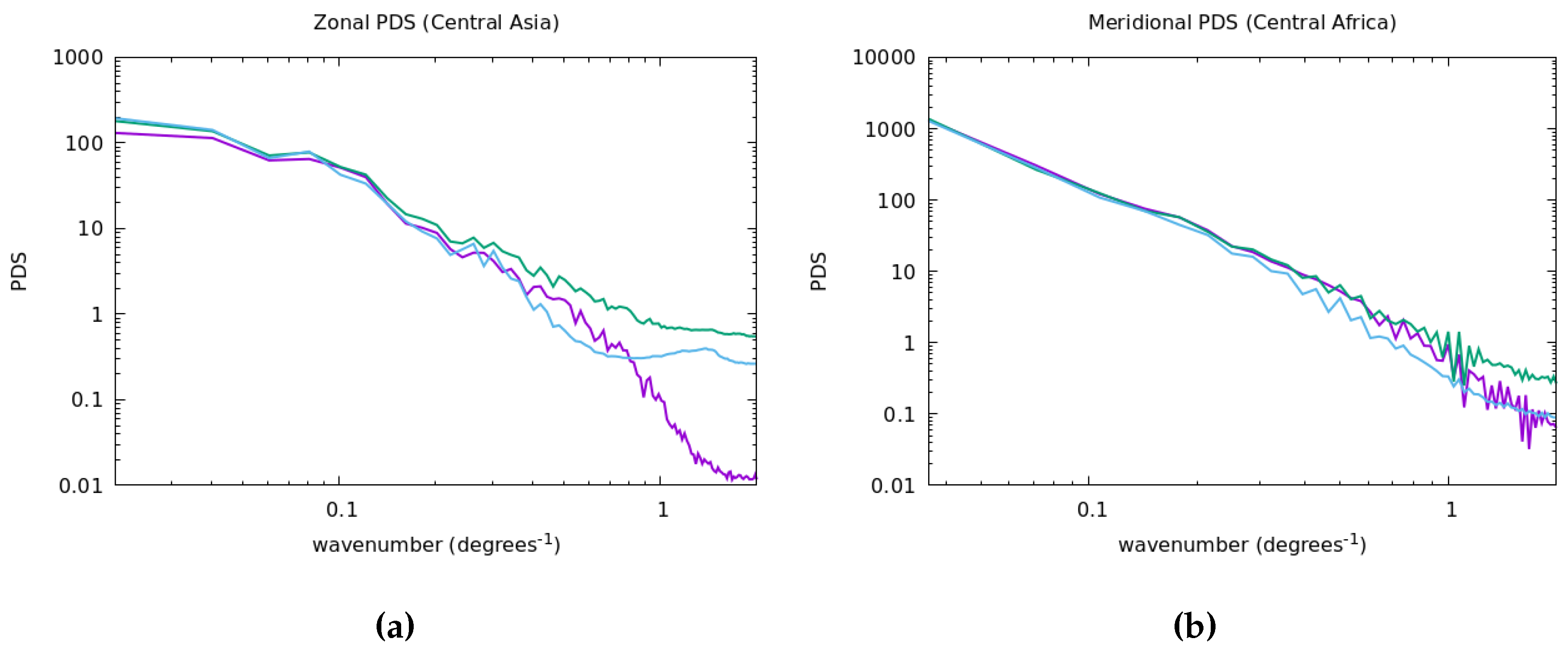
One of the required conditions to apply CTC is that the three measurements being compared must be defined over similar spatial scales. We have assessed the scales of the three TB datasets (SMAP, SMOS nominal, and SMOS NS) by analyzing their Power Density Spectra (PDS) [35]. We have computed their PDS for two large regions, differently orientated (zonal or meridional). The first kind of PDSs (labelled “Central Asia”) is defined by the zonal transects extending from 45° to 110°W; the PDS of those transects are averaged over a range of latitudes going from 40° to 60°N and over the full time extension of the maps. The second kind of PDS (labelled “Central Africa”) is defined by the meridional transects extending from 30°S to 30°N; the PDS of those transects are averaged over a range of longitudes going from 15° to 30°W and over the full time extension of the maps.
The obtained PDSs, S ( k ) , are expected to behave as a power law of the wavenumber, k. Therefore, we expect S ( k ) k β , where the value of the scaling exponent β is expected to be between 1 and 2. This means that, when representing the PDS vs. k in a log-log plot, we should observed a straight line with a slope exactly equal to β .
The behaviour of the PDS is expected to deviate from the pure power law in the presence of resolution-limiting effects. It may happen that the measurements have a certain level of white noise, so the actual behavior of the PDS would then be S ( k ) k β + η , where η is the amplitude level of the white noise, which is a constant, independent of the wavenumber k. Therefore, for wavenumbers large enough, the power-law term becomes negligible and we would then have S ( k ) η . We can determine a threshold wavenumber k 0 such that, for k < k 0 , we have with a good approximation S ( k ) k β (therefore, the physical scales are well resolved) and, for k > k 0 , we have with a good approximation S ( k ) η (therefore, the measurement is dominated by noise and no physical scales are utterly resolved). This threshold k 0 is the resolution wavenumber, which defines the resolution wavelength λ 0 = k 0 1 . Since at a wavelength we can resolve two points (one assigned to the positive part of the sinus, and the other assigned to the negative part), we can define the resolution scale as r 0 = λ 0 / 2 = ( 2 k 0 ) 1 .
Noise is the most common effect limiting the effective resolution of data, but there are others. Low-pass filtering effectively suppresses noise but lower scales as well, and therefore, it also limits the effective resolution of the data. In terms of PDS, the impact of applying a low-pass filter is evidenced by a sudden drop of value for wavelengths k beyond a given threshold value k 0 . Exactly as in the previous case, this threshold wavenumber k 0 serves to determine the effective resolution of the data.

3. Results and Discussion

3.1. Synthetic Experiments on Error-Correlated Triplets

We have defined three metrics to assess the performance of the CTC and LSETC methods:
  • Fraction of valid retrievals is the ratio of the total valid retrievals (that is, nonnegative estimates of the error variances σ δ i 2 ) to the total number of realizations. The closer to 1, the better.
  • Bias is the difference between the average of all valid estimates of the error standard deviations σ δ i and the value used for the generation of the dataset. The closer to 0, the better. It provides the bias in our estimates of σ δ i . Positive bias indicates that the error is overestimated, and negative bias indicates that it is sub-estimated.
  • Uncertainty is the standard deviation of the valid estimates of error standard deviations. The closer to 0, the better. It provides the accuracy in our estimates of σ δ i .
The results of the synthetic experiments are shown in Figure 1, Figure 2 and Figure 3. Each panel corresponds to a given value of the sampling size N (per rows). We show each one of the three metrics per columns. In all panels, the x-axis corresponds to the error correlation ρ 12 . Solid lines are for CTC, while dashed lines correspond to LSETC.
The main findings and conclusions from the analysis with synthetic data (Figure 1, Figure 2 and Figure 3) can be summarized as follows:
  • The fraction of valid points is very large even for scarce samplings ( N = 50 ) for the measurements with the largest error standard deviations. The number of valid retrievals for the “small uncorrelated case” and “large uncorrelated case” is lower for the measurement with the lowest error standard deviation: in the range of 60% for scarce sampling and increasing slowly for larger sampling sizes. CTC has in general a larger number of valid retrievals than LSETC, especially in the “small uncorrelated case” and less in the “large uncorrelated case”. The fractions of valid points for LSETC and CTC are very similar in the “equal case”.
  • Biases are not very large in the “small uncorrelated case” and “equal case”. Even for scarce samplings ( N = 50 ), they are at most about 10% of the largest error standard deviation for the CTC and about 20% for the LSETC. The situation is worse in the “large uncorrelated case”, where it has 30% of the largest error standard deviation (both for CTC and LSETC) for scarce sampling and only attains 10% for good sampling ( N = 500 ) or better. In most cases, the performance in terms of biases of CTC is better than that of LSETC.
  • The measurement with the smallest error standard deviation has always a positive bias in CTC, indicating that its error standard deviation is always overestimated. This bias is reduced rapidly as sampling size N increases. In the “equal case”, biases are negligible for the three measurements even for scarce sampling.
  • Uncertainties are small in the “small uncorrelated case” and moderate in the other two cases. In the two latest cases, we expect uncertainties to be around 10% of the largest error standard deviation even with excellent samplings ( N = 1000 ). CTC outperforms LSETC, especially in the “small uncorrelated case”.
  • From the experiments, we see that the dependence of all metrics on the value of the error correlation ρ 12 is weak in most cases. For the “small uncorrelated case”, the bias and uncertainty decrease at high correlation values for CTC, since the two measurements with larger errors become essentially the same, but in all cases, CTC outperforms LSETC. Hence, CTC is very robust independently of the degree of correlation between those errors.
Based on all previous points, we conclude that CTC is an optimal method for assessing TC errors in the triplets formed by SMOS nominal, SMOS NS, and SMAP TBs. This corresponds to the “small uncorrelated case (since the measurement with uncorrelated error, SMAP, has an error standard deviation significantly lower than the SMOS measurements). In this case, CTC outperforms LSETC in the convergence speed and in terms of bias and standard deviation. Therefore, we will take CTC as our reference triple collocation method for the characterization of radiometric errors in satellite L-band brightness temperatures over land.

3.1.1. Impact of Statistical Fluctuations on the Estimation of Intercalibration Factors

For each sampling size N, we have computed the mean and standard deviation of the intercalibration factors over the ensemble of 100,000 realizations. While the means are very close to 1 (not shown), the standard deviations are not negligible (see the log-log plot in Figure 4) and decay slowly with sampling size 1 / N . This is expected for fluctuations according to the Central Limit Theorem. The (extrapolated) value for N = 1 determines the factor multiplying 1 / N , and this factor determines the vertical positioning of the curves. As shown, those factors depend on the values of the error standard deviations and significantly differ for the different cases. The standard deviation of the intercalibration factors is typically around 0.1 for N = 50 (that is, an error of ≈10% around the right value) and even around 0.02 or 2% for N = 1000 . Notice that those curves have been obtained from simulated data assuming Gaussian distributions for both the errors and the signal. Dispersion in the estimation of the intercalibration factors could be even larger if the distribution of the signal significantly deviates from a Gaussian distribution and if the measurement errors are correlated.
We conclude that statistical fluctuations, even with moderately large sampling size, are important enough to give the false impression that the measurements are poorly intercalibrated.

3.1.2. Sensitivity Analysis of the Estimated Error Variances to Changes in the Intercalibration Factors

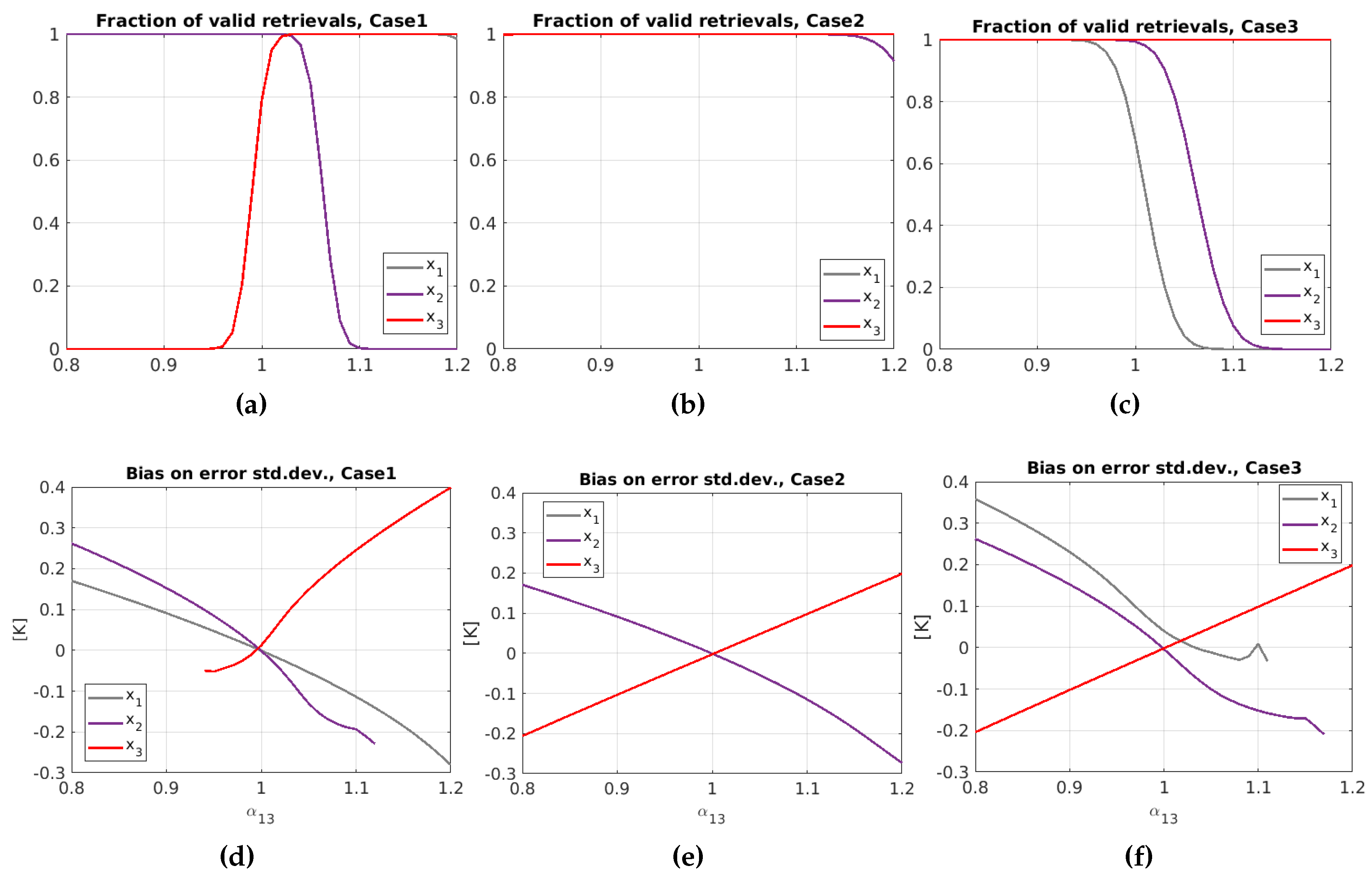
We have carried out an experiment to analyze the impact of errors in the intercalibration factors on the retrievals obtained by the application of CTC. As discussed earlier, the factors a 1 and a 2 can be adjusted to be coincident, so the only factor missing is a 3 (or the intercalibration factor α 13 ).
We have generated a series of synthetic data to assess the impact of having an intercalibration factor α 13 significantly differing from one. For that, we have computed a dataset of series for each value of α 13 between 0.8 (20% lower) and 1.2 (20% larger) in intervals of 0.01. We have generated 100,000 series of synthetic signals, each one with a sampling size of N = 500 , and the correlation coefficient between measurements 1 and 2 ( ρ 12 ) has been kept fixed to 0.5.
To assess the results, we have taken as metrics the fraction of valid retrievals and the biases of the estimates.
As shown in Figure 5, the bias is a decreasing function of α 13 for the error-correlated measurements x 1 and x 2 , while it increases for the uncorrelated measurement x 3 . For x 3 , the relation is almost perfectly linear when σ δ 3 = 0.5 (that is, the “equal” and “large uncorrelated” cases in Section 2.2). Probably, the excess or lack of signal associated to the change in the intercalibration factor is attributed to the error of x 3 measurement, with a similar change in magnitude but of opposite sign for measurements x 1 and x 2 . Therefore, the impact on the estimates of the error standard deviations will be larger when the variance of the signal (here, conventionally fixed at 1) is larger.
As evidenced by the curves of valid retrievals (bottom plots in Figure 5), when the bias induced by the change in α 13 is close to a critical value when σ δ i would go to zero, there is a sudden drop in the fraction of valid retrievals. Therefore, the number of valid retrievals is a good indicator of having problems with the intercalibration factors. The transition points depend on the ratio between the error standard deviation and one of the signal. In our figures, the drops happen at percentages of variation of the intercalibration factor that are equal to the standard deviation of the error of the affected measurement; this is not a coincidence but a consequence of the variance 1 for the signal. A signal with larger variance will have transition points at lower values of the percentage of miscalibration. When working with real signals, as the variance of the errors is typically much smaller than that of the signal, the range of admissible errors in the intercalibration factor is quite narrow in practice.

3.2. Error Characterization of Satellite L-Band Brightness Temperatures over Land

The triple collocation analysis has been performed for TB maps at H-polarization, V-polarization, and for the half of the first Stokes parameter. Only results for the latter are shown, but similar results have been obtained for the H and V polarizations.
In order to assess if the datasets resolve similar spatial scales, we have computed the PDS for the Central Asia and Central Africa regions for the three datasets (Figure 6). The three curves are very close to each other for large scales and are in relatively good agreement with the expected power law. The behaviour of the zonal transect (Central Asia) and of the meridional transect (Central Africa) are slightly different probably due to the RFI contamination over Asia, which is filtered on-board in the case of SMAP and not in SMOS. For Central Asia, the PDSs start to slightly diverge at about k = 0.3 (degrees)−1. Then, close to 1 (degrees)−1, the three curves reach their limit: both SMOS PDSs become essentially horizontal while SMAP experiences a serious drop of value, indicating that it is a smoother product. In the case of Central Africa, the three curves are packed closer together, but again, at about 1 (degrees)−1, both SMOS curves become rather horizontal while SMAP undergoes a drop, although less sharp than in the other case. We conclude that, for the three datasets, the threshold wavenumber is about 1 (degrees)−1, which means that their effective resolution is approximately the same, corresponding to 0.5°. This is consistent with the theoretical spatial resolutions for SMAP (37 km × 49 km) and SMOS (35 to 50 km).
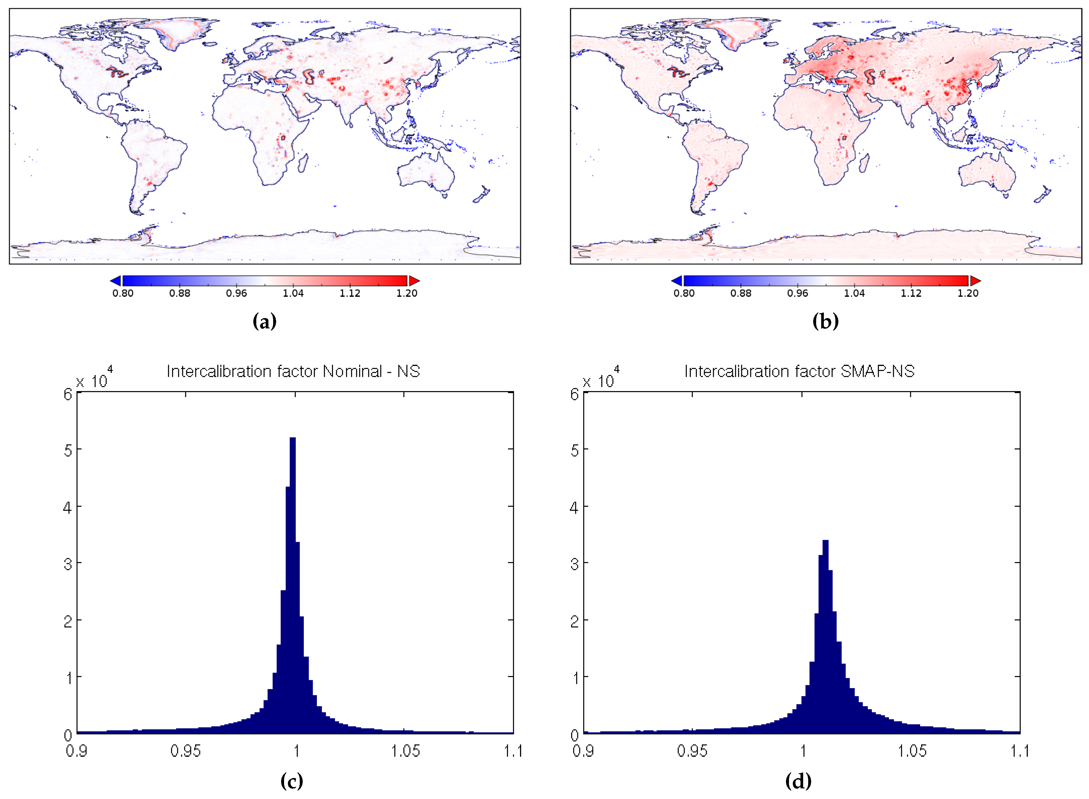
The intercalibration factors have been estimated by the ratio of the average TBs for the time-series between the two corresponding datasets. The intercalibration factor between SMOS nominal and SMOS NS ( α 12 ) is very close to the one for most of the points in the map (see the left column in Figure 7, mean value: 0.997). Differences are mainly concentrated around coastlines and ice edges, where the NS TBs are systematically higher than the nominal ones (due to known residual systematic biases present in NSv2 [36]) and in the location of RFI sources, as reported in [11]. Analyzing the ratio between SMOS NS and SMAP ( α 13 ), differences are more noticiable over Europe and China due to the higher RFI contamination in SMOS TB (see the right column in Figure 7). In any case, the global mean of α 13 is 1.014, indicating a good overall agreement between SMOS NS and SMAP measurements. Notice that the intercalibration factors are close to 1, with deviations in the expected range due to statistical fluctuations (see Section 3.1.1).
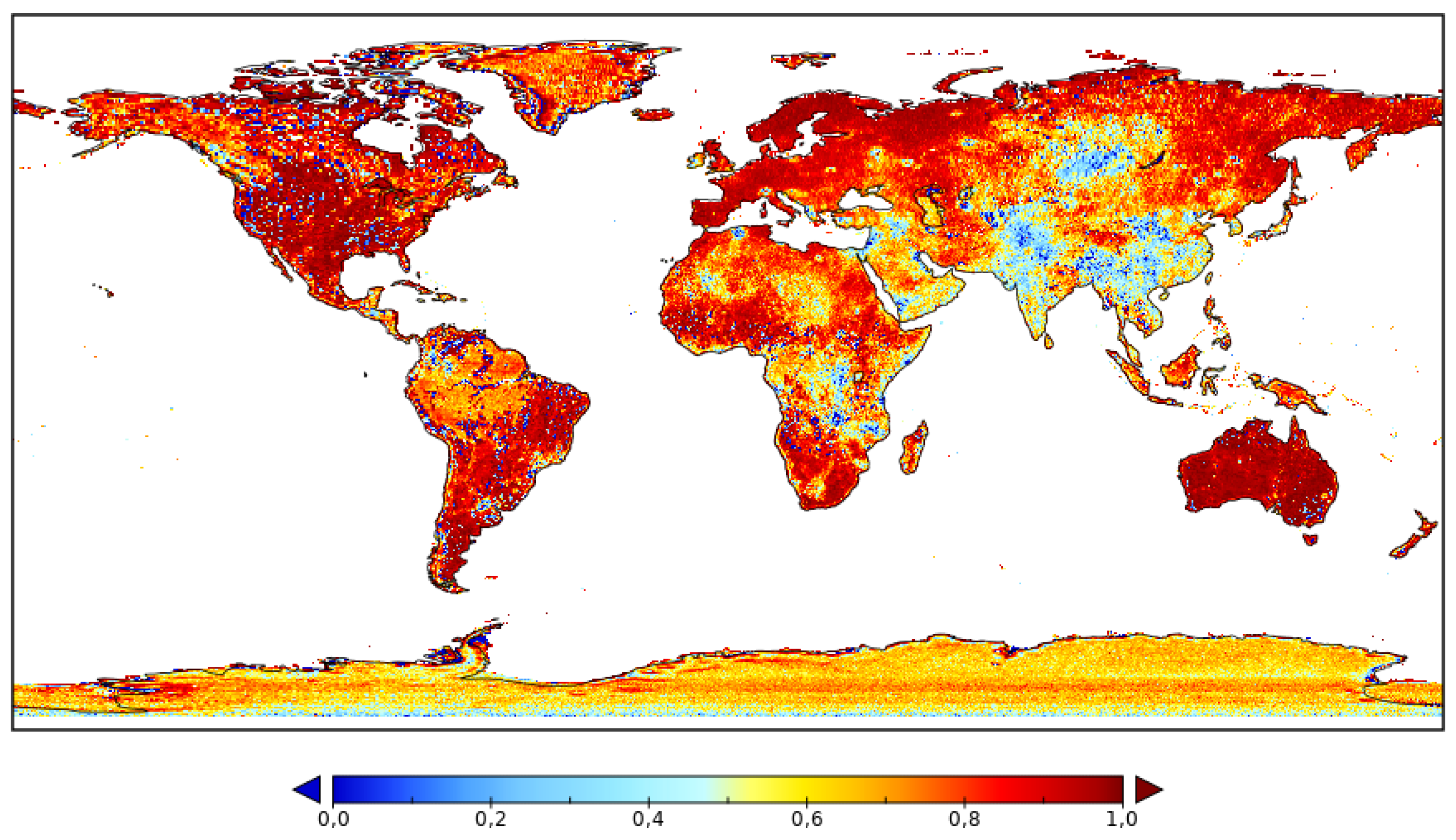
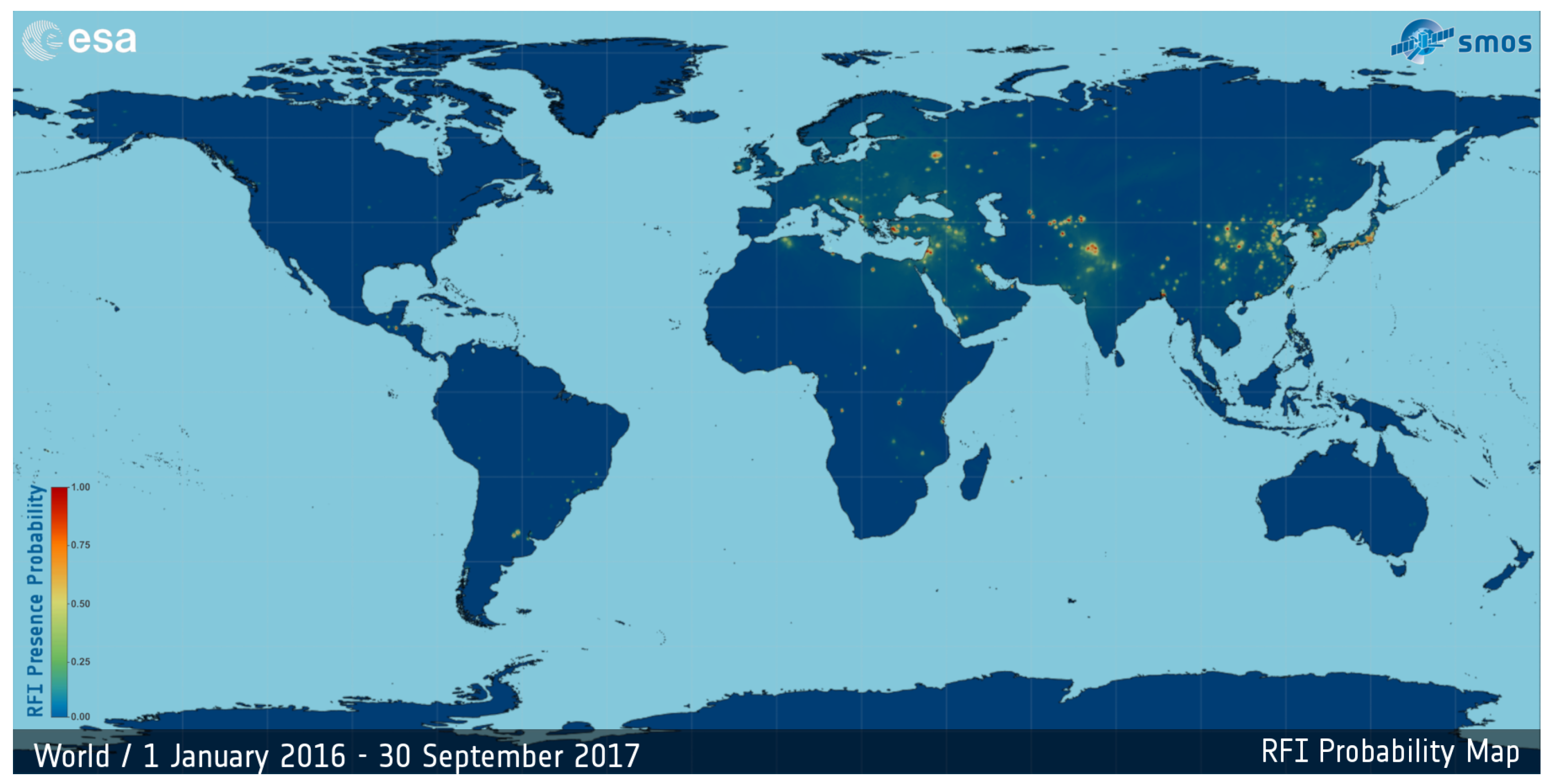
The error correlation parameter ρ 12 between the two SMOS datasets (see Figure 8) has been estimated following the equations summarized in Section 2.1.3. It can be appreciated that errors are highly correlated for most of the points: the mean correlation is 0.71, and over wide areas of the globe, ρ 12 is very close to 1 and, in all cases, positive. Those places where the correlation significantly drops seem to be related to the presence of intense RFIs, which can be corroborated looking at the map of SMOS RFI probability in Figure 9. This RFI probability has been computed following the procedure detailed in [37] for the period January 2016–September 2017.
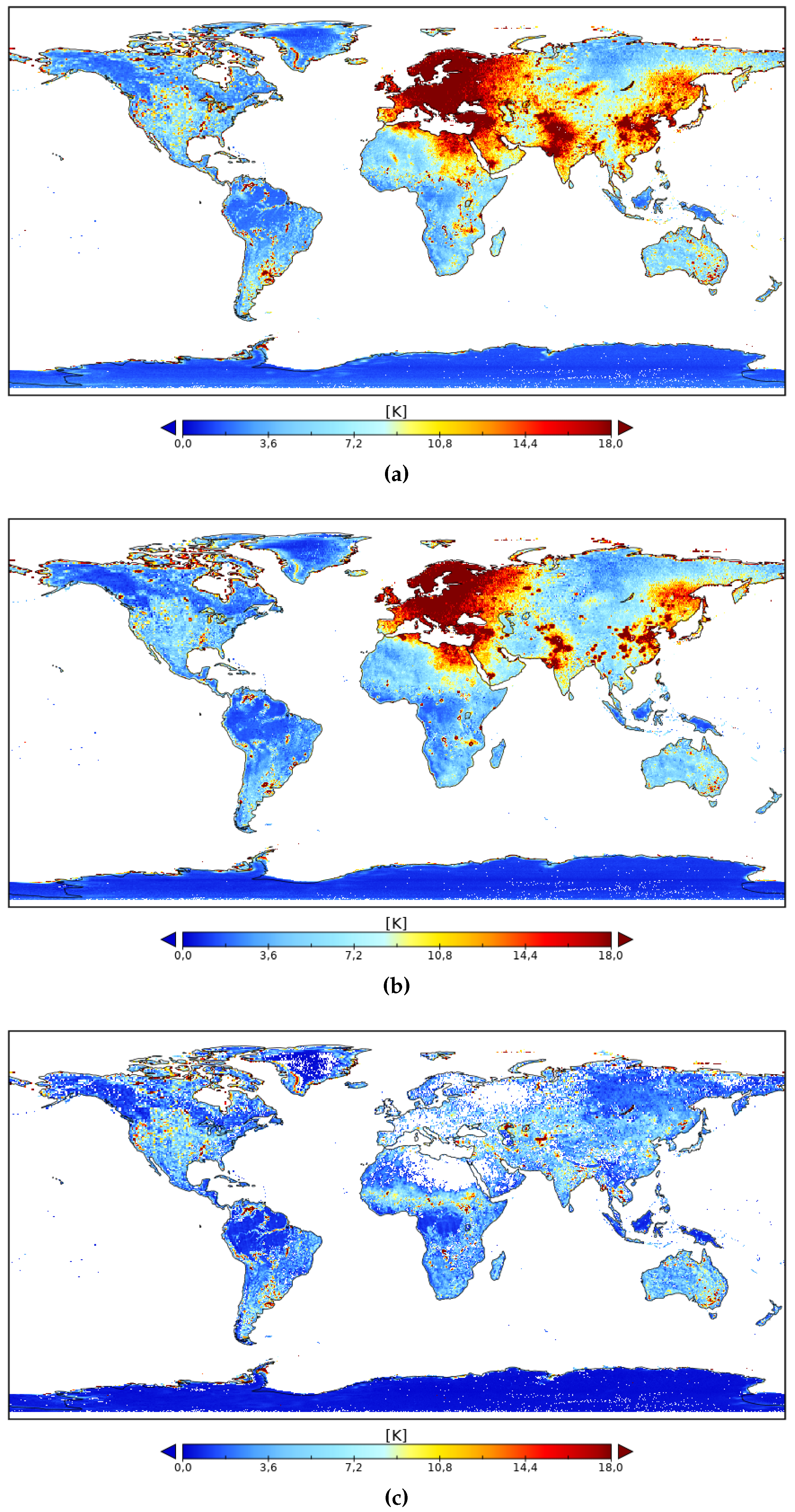
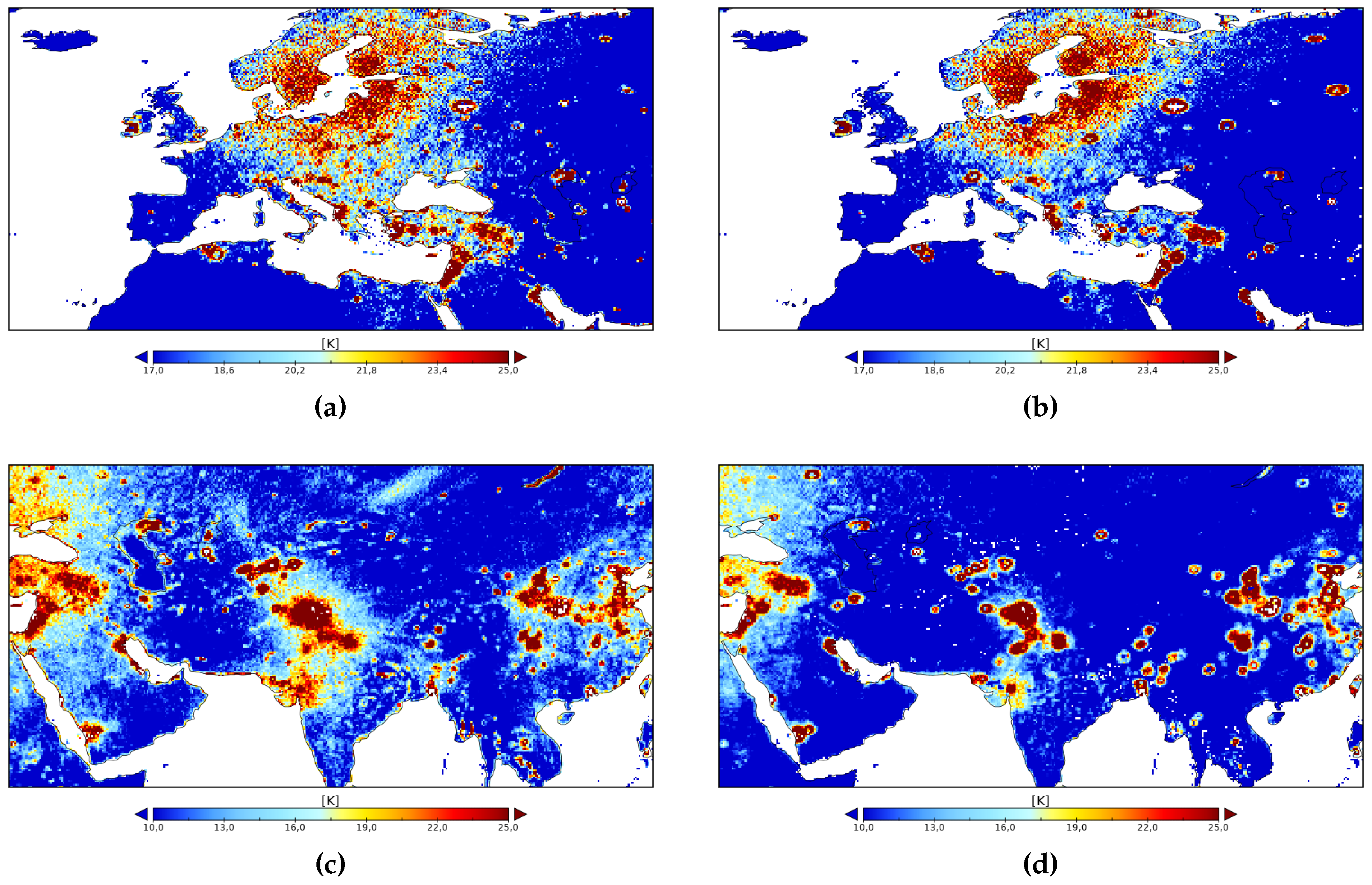
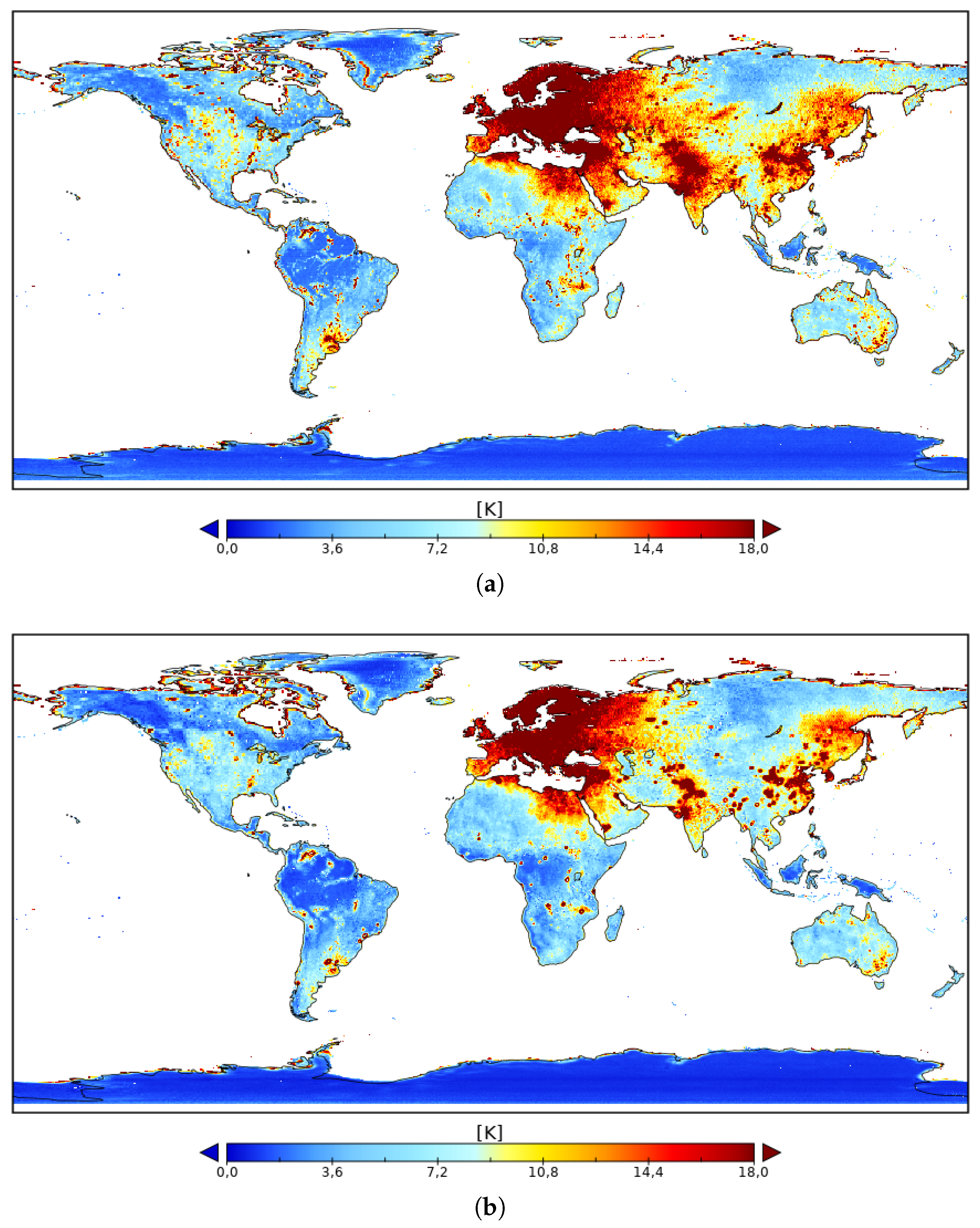
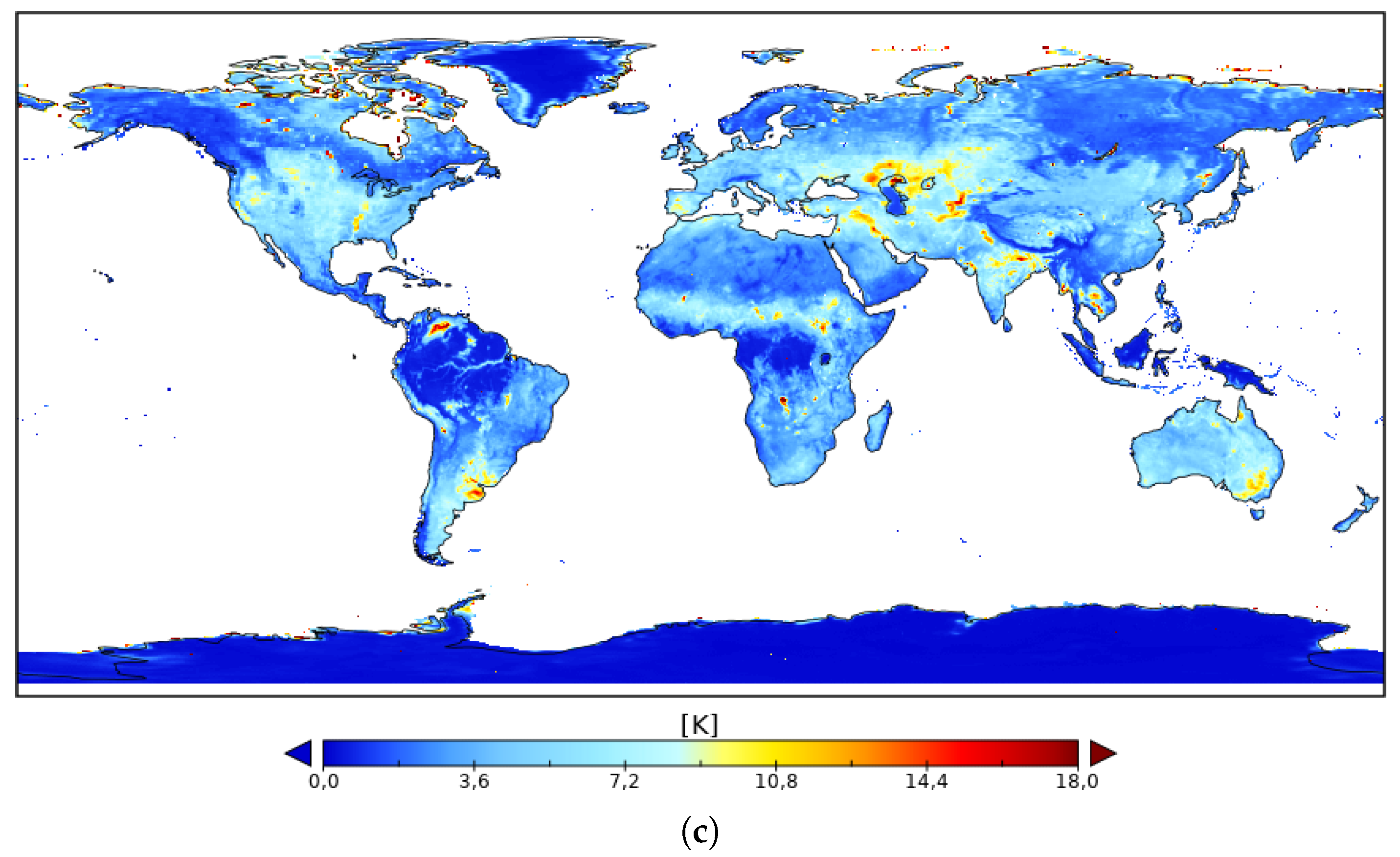
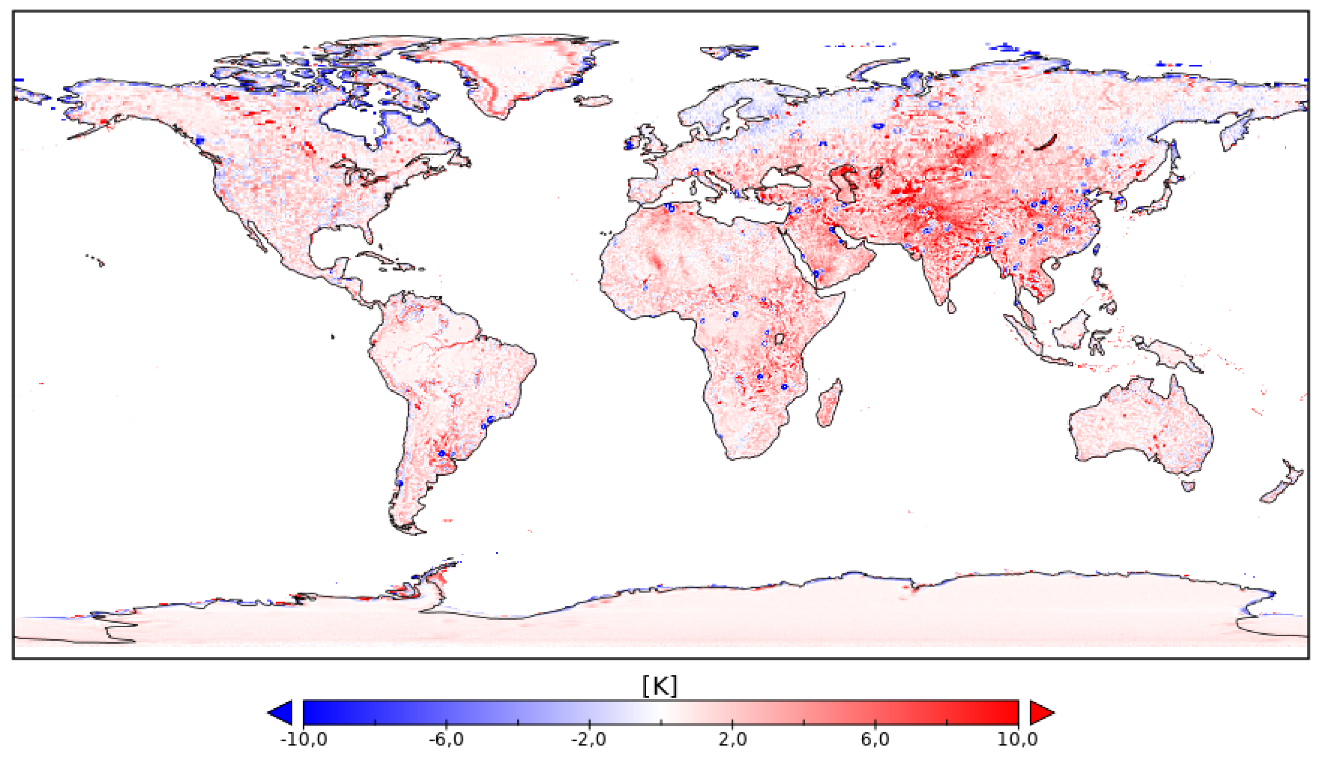
Global maps of the error standard deviation for each one of the three TB datasets are shown in Figure 10. Notice the low estimated errors over Antarctica, which can be explained by the very low temporal and spatial TB variability over that region. The application of NS has led to an overall significant reduction of TB errors with respect to SMOS nominal TB, particularly over strongly RFI-contaminated regions. NS errors are more concentrated around the locations of the RFI sources (see Figure 9). This reduction over Europe, Arabian, India, and China can be more clearly appreciated in the zoom of Figure 11. It is important to point out that the error estimation of SMAP was not valid (negative values; see Appendix A) over 15% of the gridpoints (Figure 10c). In the case of the SMOS nominal and SMOS NS, the number of data gaps (nonvalid estimates) is very low (1.02% and 1.34%, respectively). This is consistent with the findings in our experiment with synthetic data case 1 in Section 2.2. As we show below, SMAP error standard deviation is smaller than that of the other two and the number of valid retrievals is approximately 85 % for 210 samples, which is in between 60% of retrievals for N = 100 samples and approximately 80–90% for N = 500 obtained in the synthetic experiments.
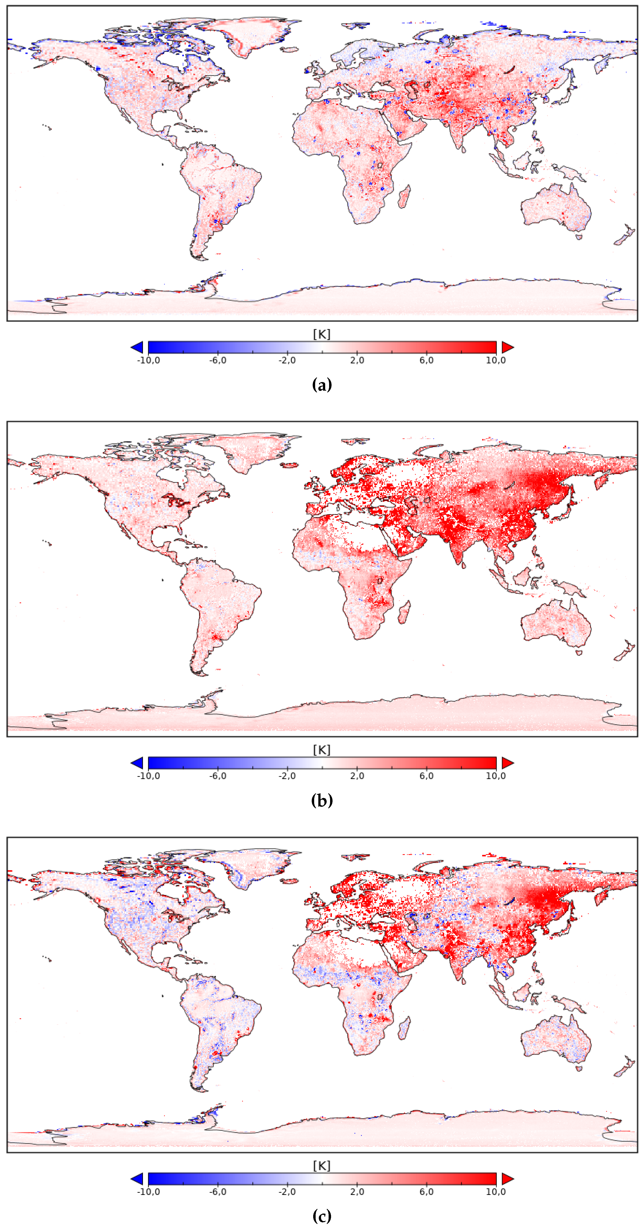
The map of the differences between the error standard deviation of SMOS nominal and SMOS NS (Figure 12a) confirms that the application of NS effectively reduces the RFI contamination over land. The exception is for gridpoints close to the coastlines and those in the locations of RFI sources (see the blue spots and their correspondence to the RFI probability map in Figure 9), which present larger errors in NS TBs. These are known limitations of NSv2, as published in [11,36]. The residual contamination in coastal (and in ice edges) gridpoints is expected to be largely reduced by applying a refined version of the NS algorithm, very recently developed to improve the performances in land/ocean/ice transitions. Looking at the difference between the error standard deviation in SMOS nominal and SMAP (Figure 12b), the highest differences are found over RFI-contaminated regions but are also noticiable over RFI-free areas. These differences are significantly reduced when analyzing the difference between the error standard deviation in SMOS NS and SMAP (Figure 12c). Errors in NS TBs are larger than those of SMAP in RFI-contaminated regions, which is expected since RFI contamination in SMAP is much more moderate thanks to its on-board digital detector back end [31,32]. For some RFI-free regions, NS leads to lower errors than SMAP (see bluish regions in Figure 12c). The smaller error standard deviation of SMAP with respect to SMOS was expected because the radiometric accuracy in the averaged SMOS incidence angle range (37.5–42.5°) is worse than that of SMAP. However, it is important to notice that SMOS final retrieved error is comparable to SMAP when considering the whole incidence angle range. What is actually significant is that, with the application of NS (which is known to lead to an improvement of the effective radiometric accuracy [11]) over certain areas, the SMOS data acquired close to SMAP incidence angle can overcome SMAP accuracy.
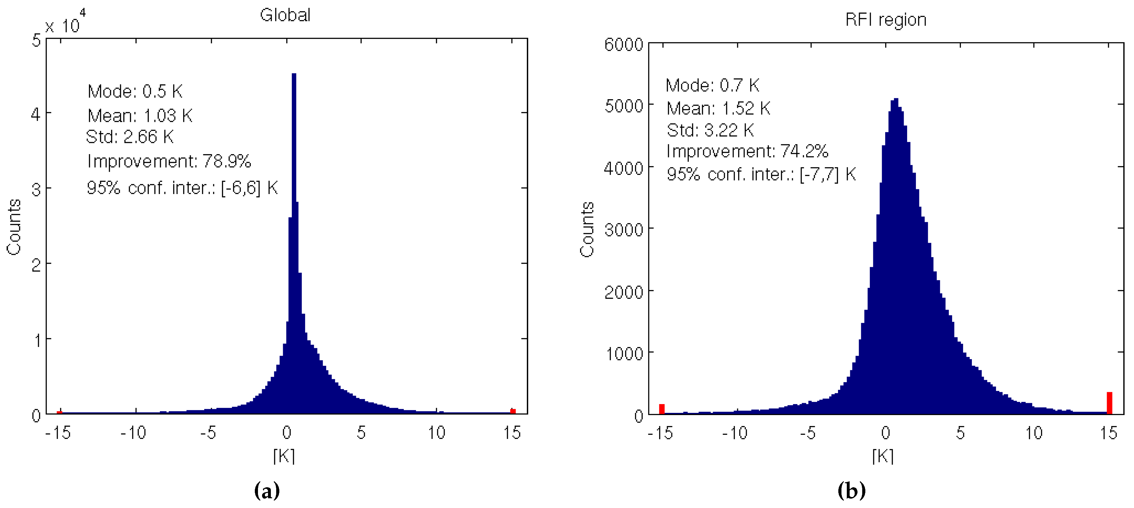
Histograms of the differences between error standard deviations of SMOS nominal and SMOS NS are shown in Figure 13a for the global map and in Figure 13b for the region that is more affected by RFI contamination, covering Europe, Asia, and north Africa (longitude range (20 W, 180 E), latitude range (10 N, 80 N)) (see Figure 9). Statistics show that NS reduces SMOS TB errors over strongly RFI-contaminated regions (mean error reduction approximately 1.5 K ) and generally improves TB quality (approximately 75% of the gridpoints over land present lower errors for NS TBs than for the nominal ones). Similar statistics are obtained when considering the global map, although the mean error reduction is decreased. The impact of NS is lower over RFI-free regions, but it is still beneficial since it reduces overall ripples in TB images.
In the case of SMAP, error estimates for 15% of the gridpoints have not converged to a meaningful value (white shading in Figure 10c). A refinement of the TC analysis is proposed in Section 3.2.1 to obtain error estimates for the global map.

3.2.1. Inferring SMAP Errors Overestimate Gaps

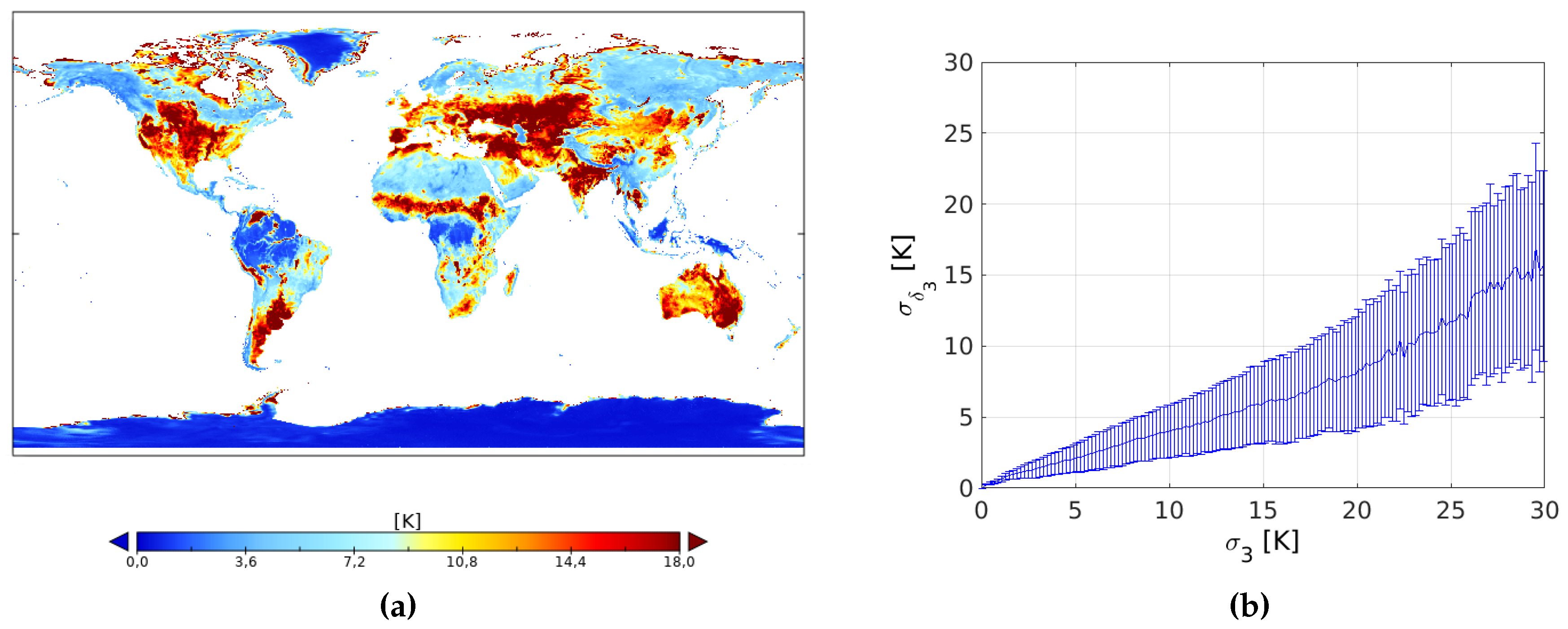
Looking at the maps of the standard deviation of the SMAP TBs (Figure 14a) and their error standard deviation (Figure 10c), it is evident that both variables are related by an increasing function. Over 85% of points have a valid estimate of σ δ 3 ; we computed the histogram of σ δ 3 conditioned by the value of σ 3 = s 3 (taking bins of 0.1 K). From this conditioned histogram, we have computed the conditioned mean and conditioned standard deviation of the relation between those two variables. The result is shown in Figure 14b; the conditioned mean represents the central value, while the conditioned standard deviation is represented as the error bars. Except for very large values of σ 3 (which are not very significant, as there are few values and therefore the relation is poorly inferred), we see a clear linear relation between both variables, although the dispersion (the error bars) is quite significant.
As a strategy to improve the estimation of σ δ 3 over the gaps, we computed the parameters of a linear regression between σ δ 3 and σ 3 . We performed a weighted least square fit, where each value of σ 3 was weighted by the inverse of the conditioned variance. The resulting linear relation is σ δ 3 = a σ 3 , where the empirical value of a is a = 0.42 .
Assuming the linear relation between the error variance and the measurement variance, the variance of the geophysical signal can be estimated as follows:
σ θ 2 = s 3 σ δ 3 2 = ( 1 a 2 ) s 3
Then, the covariance of the combined SMOS and SMAP variables, s 23 , which is in fact an estimate of σ θ 2 , can be substituted in Equation (8) by the value yielded by Equation (10). Error standard deviations for the three measurements have been computed (hereafter, adjusted error standard deviations) with the proposed refinement (Figure 15). Adjusted error estimates are very similar to the error standard deviations estimated in the initial analysis (Section 3.2) but with almost complete spatial coverage. Note that mean adjusted errors have slightly increased with respect to the previous mean error estimates (see the mean values in the captions of Figure 10 and , respectively) and with an improved coverage (less gaps).
NS TBs show an overall decrease of errors both in RFI-contaminated regions and over RFI-free regions (see Figure 16). Statistics in the histograms of Figure 17 confirm that the mean error reduction of SMOS NS with respect to SMOS nominal TBs is very similar to the one obtained in the first iteration of CTC (Section 3.2, Figure 13). NS leads to an improvement of the TB quality in 79% of the gridpoints over land.

4. Conclusions

A new formulation of the triple collocation analysis has been developed for the specific case of three datasets resolving similar spatial scales and presenting correlated errors for two of them. The CTC method has been designed to be as less data demanding as possible, and it has been first assessed using synthetic data. The performance of this method has been compared with the LSETC: CTC attains a higher fraction of valid retrievals and outperforms the classical LSETC in terms of biases and uncertainties of the error estimates, specially for scarce to moderate sampling sizes. In the “equal case” (similar errors in the three measurements) and in the “large uncorrelated case” (the measurement with uncorrelated error has an error standard deviation significantly higher than the other two), both methods perform quite similar, although CTC attains a higher fraction of valid retrievals, specially in scarce samplings.
This methodology can be particularly beneficial for the error characterization of variables for which getting measurement systems with uncorrelated errors is challenging or not feasible. The method is thought to be especially suited for its application to triplets of remote sensing maps that resolve similar spatial scales, where having three collocated, completely independent remote sensing maps is unlikely.
As an example of the application of this method, we have used it for the characterization of radiometric errors in L-band brightness temperatures over land. The triplets formed by SMAP, SMOS nominal, and SMOS NS TBs have been specifically analyzed for evaluating NS performances over land as an RFI mitigation technique. CTC method has been shown to provide spatial maps of errors within a reasonable margin of uncertainty even with a moderate sampling size.
The triple collocation analysis has revealed that TB errors are significantly reduced when NS is applied with respect to SMOS nominal data, attaining a mean error reduction of approximately 1.5 K in strongly RFI-contaminated regions and approximately 1 K globally. The application of NS has been shown to improve the quality of TBs in 79 % of the gridpoints of the map. Most of the gridpoints where nominal TBs present lower errors than NS are in the precise locations of the RFI sources (measurements that in any case will be discarded before geophysical retrieval) and along the coastline. The increase of the systematic biases very close to the coasts and ice edges is a known performance issue with NSv2 [36]. Precisely, a refined version of NS focused on reducing these systematic biases in the coasts has been recently developed, and it is currently under extensive validation.
The extension of the present analysis to global TB maps (including ocean and ice) is ongoing, with the aim to assess the NS impact on TB independently on the target. The same CTC methodology can be applied to the retrieved geophysical parameters (both soil moisture and ocean salinity). We are currently working in the error characterization of different L-band sea surface salinity products (including SMAP, SMOS, and reanalysis data) with promising results [38].
The CTC technique is currently being used by the SMOS Level 1 Expert Support Laboratories as a metric for assessing the performance at TB level of the next versions of the SMOS L1 processor with respect to the current one. The TC presented in this work is a very valuable tool since it can provide insights about the improvements/limitations of the changes proposed at L1 without the need for a forward model or for further retrieval of the geophysical parameters and validation of them. In this context, the performances of a new extrapolating technique of the TB frequencies outside the star coverage of SMOS to mitigate RFI contamination effects are also being evaluated [39].

Author Contributions

Conceptualization: V.G.-G., A.T. and E.O.; methodology: V.G.-G., A.T., C.G.-H., J.M. and E.O.; software: V.G.-G., A.T. and J.M.; validation: V.G.-G., E.O., C.G.-H. and R.O.; formal analysis: V.G.-G., A.Y. and J.M.; interpretation of results: all authors; writing—original draft preparation: V.G.-G. and A.T.; and writing—review and editing: E.O., C.G.-H., R.O. and M.M.-N. All authors have read and agreed to the published version of the manuscript.

Funding

This research was funded by the Spanish Ministry of Economy and Competitiveness, through the National R+D Plan under L-Band Project ESP2017-89463-C3-1-R and by previous grants from the European Space Agency through the contract of SMOS Expert Support Laboratories Level 1 (SMOS-P7-DME-COM-CCN05-E-R) and the CCI+ Sea Surface Salinity project. This work is a contribution to CSIC Thematic Exploitation Platform TELEDETECT.

Acknowledgments

The authors would like to thank Ekhi Uranga and Alvaro Llorente from ESAC (European Space Astronomy Centre)/ESA for providing the SMOS RFI probability data.

Conflicts of Interest

The authors declare no conflict of interest.

Appendix A. Triple Collocation with Two Error-Correlated Datasets: Theoretical Basis

Let us assume that we have a series of three independent linear measurements ( x 1 , x 2 , and x 3 ) of the same quantity θ :
x i = a i θ + b i + δ i i = 1 , 2 , 3
We want to estimate the standard deviation of the errors δ i that we denote by σ δ i , under a given set of assumptions. As we have an explicit independent term b i , we consider the errors to be unbiased, so δ i = 0 . We further assume that the errors are uncorrelated from the physical quantity, θ δ i = 0 . We assume that errors 1 and 2 are correlated, with a covariance ϕ 12 = δ 1 δ 2 , but the errors of these two variables are completely uncorrelated from the error of measurement 3 ( δ 1 δ 3 = 0 and δ 2 δ 3 = 0 ).
It is often assumed that the calibration factors a i are known or can be estimated by independent methods previously to the triple collocation (then, without loss of generality, taken as 1) in order to simplify the problem. In this case, we have five unknowns: the standard deviation of the physical signal, σ θ ; the three standard deviations of the errors, σ δ i (for i = 1, 2, 3); and the covariance of errors 1 and 2, ϕ 12 . To estimate those standard deviations and covariance, we have six equations, given by the six order-2 statistical quantities that we can derive from the measurements: the three measurement variances s i = x i 2 x i 2 and the three measurement covariances s i j = x i x j x i x j . Therefore, our problem would be defined by an overdetermined system: we have one more equation than needed. We must exploit this redundancy in order to ensure rapid convergence of the estimators of the error standard deviations, which would allow us to have reliable estimates even with datasets of limited sampling size.
Let us start by a simplified case, namely when the error covariance of 1 and 2 vanishes, ϕ 12 = 0 .

Appendix A.1. Case of Three Variables with Independent Measurement Errors

In this case, the three variables are equal. From Equation (A1), it trivially follows that
s i = a i 2 σ θ 2 + σ δ i 2 ; s i j = a i a j σ θ 2
A very coarse estimate of the errors could be obtained if we consider that all calibration factors a i are equal to 1 (after a proper normalization) and just estimating the signal variance σ θ 2 from any measurement covariance, for instance, s 12 ; we would therefore have σ δ i 2 = s i s 12 . However, statistical fluctuations due to finite sampling would make this kind of estimator noisy and less reliable. A better estimation of the signal variance could be obtained by averaging all the covariances, σ θ ^ 2 = 1 3 ( s 12 + s 13 + s 23 ) and then by applying σ δ i 2 = s i σ θ ^ 2 . Although this is a better estimate, it is also very affected by the fluctuations associated to finite sampling and particularly by errors in the calibration factors a i .
If we assume that the calibration factors are not known, it is still possible to estimate the error variances, and thus, any possible error in the calibration factors can be neglected. In such a case, we have more unknowns than equations. It is easy to verify that the final expression for the most general case is as follows:
σ δ 1 2 = s 1 s 12 s 13 s 23 σ δ 2 2 = s 2 s 12 s 23 s 13 σ δ 3 2 = s 3 s 13 s 23 s 12
An additional advantage of this expression is that it makes optimal use of the statistics, so the fluctuations due to finite sampling are smaller and the estimates are more accurate.
We can estimate the intercalibration factors α i j = a i / a j by dividing the covariances of both variables with the third one:
α i j = s i k s j k w i t h k i , j

Appendix A.2. Two Measurements with Correlated Errors but Uncorrelated from a Known Third Measurement: Least Squared Error Triple Collocation

One of the approaches that allows us to apply the TC in the case of two measurements with correlated errors but uncorrelated from the error of the third one is the least squares solution, which minimizes the squared error of the estimates [9]. Assuming that all calibration factors a i are equal to 1, we can write a very simple linear system relating the 6 order-2 moments of the measurements with 5 unknowns ( σ θ 2 , σ δ 1 2 , σ δ 2 2 , σ δ 3 2 , and ϕ 12 ) in the following way:
s 1 = σ θ 2 + σ δ 1 2 s 2 = σ θ 2 + σ δ 2 2 s 3 = σ θ 2 + σ δ 3 2 s 12 = σ θ 2 + ϕ 12 s 13 = σ θ 2 s 23 = σ θ 2
Defining the vectors s t = ( s 1 s 2 s 3 s 12 s 13 s 23 ) and Ω t = ( σ θ 2 σ δ 1 2 σ δ 2 2 σ δ 3 2 ϕ 12 ) , the equation above can be written as follows:
s = A Ω
where A is a 6 × 5 matrix given by the following:
A = 1 1 0 0 0 1 0 1 0 0 1 0 0 1 0 1 0 0 0 1 1 0 0 0 0 1 0 0 0 0
Notice that this is an overdetermined system, so only if the order-2 moments of the measurements are perfectly well determined will there be a solution. In general, fluctuations associated with having finite samples of data will lead to an incompatible linear system with no algebraic solution. The least squared error estimate is based on minimizing the error of the estimates [5], and it equates to applying a simple pseudo-inverse to Equation (A6):
Ω = A t A 1 A t s
Applying the least squared error estimate, Equation (A8), to our matrix A , Equation (A7), we have
A t A = 6 1 1 1 1 1 1 0 0 0 1 0 1 0 0 1 0 0 1 0 1 0 0 0 1
and
( A t A ) 1 A t = 0 0 0 0 1 2 1 2 1 0 0 0 1 2 1 2 0 1 0 0 1 2 1 2 0 0 1 0 1 2 1 2 0 0 0 1 1 2 1 2
from where we obtain the least squared error solution, given by
σ θ 2 = 1 2 ( s 13 + s 23 ) σ δ 1 2 = s 1 1 2 ( s 13 + s 23 ) σ δ 2 2 = s 2 1 2 ( s 13 + s 23 ) σ δ 3 2 = s 3 1 2 ( s 13 + s 23 ) ϕ 12 = s 12 1 2 ( s 13 + s 23 )
As a matter of fact, the least squared error solution, Equation (A11), is just one the possible solutions to the system of equations posed in Equation (A5) because it is an overdetermined system in which one of the equations must be eliminated (directly or by a proper combination of all equations); in fact, the LSE equation is just the solution of the determined system obtained by averaging the last two equations of Equation (A5). While, by construction, the LSE solution grants that the average error is minimized, it does not ensure that the convergence with respect to the number of samples is the fastest one. This is because some of the estimated error variances can be negative and must then be discarded, slowing the convergence. A possible way to circumvent this problem is to look for a different solution in which we aim to have as many positive estimates of the error variances as possible. This is precisely the basis of our CTC method.

Appendix A.3. Two Measurements with Correlated Errors but Uncorrelated from a Known Third Measurement: Correlated Triple Collocation

Let us now suppose that ϕ 12 0 . We will apply the expression for estimating the error variances when they are completely uncorrelated, Equation (A3), to obtain a first estimate of the error variances. We will denote those estimates by ω i . Applying Equation (A3), we have the following:
ω 1 = σ δ 1 2 a 1 a 2 ϕ 12 ω 2 = σ δ 2 2 a 2 a 1 ϕ 12 ω 3 = σ δ 3 2 + a 3 2 σ θ 2 a 1 a 2 σ θ 2 + ϕ 12 ϕ 12
Given that the intercalibration factor α 12 = a 1 a 2 can be computed directly from the covariances of x 1 and x 2 with x 3 ( α 12 = s 13 / s 23 ), we can use it to recalibrate the variable x 2 , so that we can assume without loss of generality that a 1 = a 2 and the error estimates are then simpler:
ω 1 = σ δ 1 2 ϕ 12 ω 2 = σ δ 2 2 ϕ 12 ω 3 = σ δ 3 2 + a 3 2 σ θ 2 a 1 2 σ θ 2 + ϕ 12 ϕ 12
We look for a linear transformation of x 1 and x 2 into two new variables x 1 and x 2 with errors δ 1 and δ 2 that are uncorrelated. The linear transformation will be defined by means of a 2 × 2 matrix U ,
U = u 11 u 12 u 21 u 22
The variables x 1 and x 2 are defined as follows:
x 1 = u 11 x 1 + u 12 x 2 x 2 = u 21 x 1 + u 22 x 2
Substituting the expressions of the variables x 1 in functions of θ and δ i , we obtain
x 1 = [ ( u 11 + u 12 ) a 1 ] θ + [ u 11 b 1 + u 12 b 2 ] + [ u 11 δ 1 + u 12 δ 2 ] = a 1 θ + b 1 + δ 1 x 2 = [ ( u 21 + u 22 ) a 1 ] θ + [ u 21 b 1 + u 22 b 2 ] + [ u 21 δ 1 + u 22 δ 2 ] = a 2 θ + b 2 + δ 2
where the square brackets in the center equations stand for the corresponding variables in the rightmost equations. The variables x 1 and x 2 will be error-decorrelated if δ 1 and δ 2 are uncorrelated. Therefore, let us analyze the covariance of δ 1 and δ 2 ; it can be expressed in terms of σ δ 1 , σ δ 2 , and ϕ 12 as follows:
δ 1 δ 2 = u 11 u 21 σ δ 1 2 + u 12 u 22 σ δ 2 2 + ( u 11 u 22 + u 12 u 21 ) ϕ 12
Using the expression for the error variance estimates in Equation (A13), we obtain the following:
δ 1 δ 2 = u 11 u 21 ω 1 + u 12 u 22 ω 2 + ( u 11 u 21 + u 12 u 22 + u 11 u 22 + u 12 u 21 ) ϕ 12
If we impose that
u 11 u 21 + u 12 u 22 + u 11 u 22 + u 12 u 21 = ( u 11 + u 12 ) ( u 21 + u 22 ) = 0
then the covariance of δ 1 and δ 2 depends only on known quantities ( ω 1 and ω 2 ). Therefore, the elements of the matrix U can be tuned to ensure that this error covariance is cancelled.
One possible choice of U is the following one:
U = 1 1 ω 2 ω 1 + ω 2 ω 1 ω 1 + ω 2
which is quite convenient as its determinant is exactly equal to 1, and then, the resulting variables after applying the linear transformation have the same order of magnitude. Besides, with this selection of variables, x 1 = x 1 x 2 (see Equation (A15)) only contains the error terms.
Therefore, the inverse of the U matrix yields the following:
U 1 = ω 1 ω 1 + ω 2 1 ω 2 ω 1 + ω 2 1
If we now define the variables x 1 , x 2 , and x 3 such that the first two are given by Equation (A16) with the particular choice of U given by Equation (A20) and x 3 = x 3 , we will be able to estimate the error variances of those three variables, obtaining the error variances of δ 1 , δ 2 , and δ 3 = δ 3 . If we denote these three variances by σ δ 1 2 , σ δ 2 2 , and σ δ 3 2 , we can compute the values of the error variances of the original variables by applying the rule of transformation for covariance matrices:
σ δ 1 2 ϕ 12 ϕ 12 σ δ 2 2 = U 1 σ δ 1 2 0 0 σ δ 2 2 U 1 t = ω 1 2 ( ω 1 + ω 2 ) 2 σ δ 1 2 + σ δ 2 2 ω 1 ω 2 ( ω 1 + ω 2 ) 2 σ δ 1 2 + σ δ 2 2 ω 1 ω 2 ( ω 1 + ω 2 ) 2 σ δ 1 2 + σ δ 2 2 ω 2 2 ( ω 1 + ω 2 ) 2 σ δ 1 2 + σ δ 2 2
and
σ δ 3 = σ δ 3
Notice that, as far as σ δ 1 2 and σ δ 2 2 are positive, the shape of Equation (A22) ensures that σ δ 1 2 and σ δ 2 2 are also positive. As a bonus, we obtain an estimate of ϕ 12 , the error covariance of variables x 1 and x 2 .
In order to compute the error variances of x i , we cannot directly apply Equation (A3) because our choice of matrix U verified that u 11 + u 12 = 0 and, thus, according to Equation (A16), we have that a 1 = 0 , that is, x 1 does not depend on θ . This makes s 13 = s 23 = 0 , which means some fractions in Equation (A3) are ill-defined. Looking at the second-order moments of the variables x i , we have that they can be related to the prime error variances:
s 1 = σ δ 1 2 s 2 = a 2 2 σ θ 2 + σ δ 2 2 s 3 = a 3 2 σ θ 2 + σ δ 3 2 s 12 = 0 s 13 = 0 s 23 = a 2 a 3 σ θ 2
Notice that, for our choice of U , we have that u 21 + u 22 = 1 and this implies, reading Equation (A16), that a 2 = a 2 = a 1 (the last equality assumed at the beginning of this section, although as we explained, a 2 can be adjusted to verify this condition). Therefore, we can estimate the prime error variances from the prime moments:
σ δ 1 2 = s 1 σ δ 2 2 = s 2 α 23 s 23 σ δ 3 2 = s 3 1 α 23 s 23
where we have used a 3 = a 3 and α 23 = a 2 / a 3 . We can only solve for σ δ 2 and σ δ 3 if we assume that a 1 = a 2 = a 2 = a 3 = a 3 . Therefore, the problem of two correlated error variances can be solved if we assume that the three variables have the same scale calibration. Notice also that, by construction, the three estimates of error variances given in Equation (A24) must be positive.
Hence, once the prime moments are known, we can compute the prime error variances using Equation (A24) and we can finally compute the original error variances and the covariance between errors 1 and 2 using Equations (A22) and (A23). Therefore, to proceed, we need to express the moments of the prime variables in terms of those of the original variables by looking at the definition of Equation (A16):
s 1 = u 11 2 s 1 + u 12 2 s 2 + 2 u 11 u 12 s 12 s 2 = u 21 2 s 1 + u 22 2 s 2 + 2 u 21 u 22 s 12 s 3 = s 3 s 12 = u 11 u 21 s 1 + u 12 u 22 s 2 + ( u 11 u 22 + u 12 u 21 ) s 12 s 13 = u 11 s 13 + u 12 s 23 s 23 = u 21 s 13 + u 22 s 23
For our particular choice of the matrix U, Equation (A20), we have
s 1 = s 1 + s 2 2 s 12 s 2 = ω 2 2 ( ω 1 + ω 2 ) 2 s 1 + ω 1 2 ( ω 1 + ω 2 ) 2 s 2 + 2 ω 1 ω 2 ( ω 1 + ω 2 ) 2 s 12 s 3 = s 3 s 12 = ω 2 ω 1 + ω 2 s 1 ω 1 ω 1 + ω 2 s 2 + ω 1 ω 2 ω 1 + ω 2 s 12 s 13 = s 13 s 23 s 23 = ω 2 ω 1 + ω 2 s 13 + ω 1 ω 1 + ω 2 s 23
The notation can be simplified to ease the use of collocated triple collocation; we can work out Equations (A22)–(A25) to a more usable form, expressing them in terms of the variances of the measurements s i and their covariances s i j . Let us define the variables u and v (that correspond to the previous u 21 and u 22 ):
u = s 2 s 12 s 1 + s 2 2 s 12 ; v = s 1 s 12 s 1 + s 2 2 s 12
which is the result of substituting the actual values of ω 1 and ω 2 . Then, we have
s 1 = s 1 + s 2 2 s 12 s 2 = u 2 s 1 + v 2 s 2 + 2 u v s 12 s 23 = u s 12 + v s 23
and the estimates of the error variances are given by
σ δ 1 2 = v 2 s 1 + s 2 s 23 σ δ 2 2 = u 2 s 1 + s 2 s 23 σ δ 3 2 = s 3 s 23 ϕ 12 = u v s 1 + s 2 s 23

Appendix A.4. Discussion on the Quality of the Error Estimates Using Correlated Triple Collocation

When data is scarce, we can have significant statistical fluctuations depending on the distribution of the error and of the signal itself. A statistical fluctuation is a large deviation from the mean value of a variable. From a statistical point of view, a statistical fluctuation can be viewed as a random variable caused by the particular sample of the data we are taking. Fluctuations tend to be smaller as we average larger and larger amounts of data, with the typical amplitude of a fluctuation as the inverse of the square root of the amount of averaged data.
Statistical fluctuations can make the estimates of error variances in TC negative, something that may happen when the amplitude of the statistical fluctuation is larger than the variance of any or all of the errors. A negative estimate for a variance must be interpreted as that value of the variance not being estimated at that level of fluctuation. This makes the estimation of the error variance harder when this error variance is much smaller than the variance of the signal itself or the variances of the other errors. In extreme cases, due to the coupling among all moments appearing in TC equations, the estimate of all error variances can be impossible.
The equations introduced in Appendix A.3 have been designed precisely to ensure that a maximum number of estimated error variances are positive by construction. This design makes our method less sensitive to statistical fluctuations and therefore best suited for the analysis of limited samples of data. Otherwise said, our method has fast convergence with the sampling size to the real values of the error variances (see the synthetic results in Section 2.2). As we will show in the following, we can grant that at least two of the three prime variables have positive estimates of their error variances.
First of all, it is worth noting that the estimators of the original error variances will always be positive as far as the estimated prime error variances are positive, disregarding the actual values of ω 1 and ω 2 . This is a consequence of Equations (A22) and (A23).
By construction, the estimate of σ δ 1 2 will always be a positive value, as it is equal to the second-order moment of the prime variable 1, s 1 . However, Equation (A24) may yield negative values for the estimates of σ δ 2 2 or σ δ 3 2 . This may happen because the determination of the second-order moments of the variables are computed with finite samples of data, and as the variance of the error is typically much smaller than that of the signal, a small finite-size fluctuation can lead to a slightly negative value. In the case of σ δ 2 2 and σ δ 3 2 , it happens that, sometimes, s 23 is slightly greater than s 2 or s 3 , making one of the estimators of prime error variances negative. While this problem decreases as the sampling size grows, it would be convenient to filter out invalid points. In the case of α 23 = 1 (that we will assume hereafter), σ δ 2 2 + σ δ 3 2 = s 2 + s 3 2 s 23 = σ x 2 x 3 2 > 0 , so at least one of the two last estimators of the prime error variances will be positive. This means that, out of the three prime error variance estimators, at most, one can be negative. In practice, this reduces the number of cases in which no estimate is found and makes our estimates more robust.
As a filtering strategy, when presenting a map of error variances, we will discard those points for which the estimate of the error variance (not the prime error variance) is negative. Therefore, the points in the error variance maps may be different. Typically the variable with the lower error variance is more affected by this problem than the others.

References

  1. Stoffelen, A. Toward the true near-surface wind speed: Error modeling and calibration using triple collocation. J. Geophys. Res. 1998, 103, 7755–7766. [Google Scholar] [CrossRef]
  2. Lin, W.; Portabella, M.; Stoffelen, A.; Vogelzang, J.; Verhoef, A. On mesoscale analysis and ASCAT ambiguity removal. Q. J. R. Meteorol. Soc. 2016, 142, 1745–1756. [Google Scholar] [CrossRef] [Green Version]
  3. Dorigo, W.A.; Scipal, K.; Parinussa, R.M.; Liu, Y.Y.; Wagner, W.; de Jeu, R.A.M.; Naeimi, V. Error characterisation of global active and passive microwave soilmoisture datasets. Hydrol. Earth Syst. Sci. 2010, 14, 2605–2616. [Google Scholar] [CrossRef] [Green Version]
  4. Pierdicca, N.; Fascetti, F.; Pulvirenti, L.; Crapolicchio, R.; Muñoz-Sabater, J. Quadruple Collocation Analysis for Soil Moisture Product Assessment. IEEE Geosci. Remote Sens. Lett. 2015, 12, 1595–1599. [Google Scholar] [CrossRef]
  5. Gruber, A.; Su, C.H.; Crow, W.T.; Zwieback, S.; Dorigo, W.A.; Wagner, W. Estimating error cross-correlations in soil moisture data sets using extended collocation analysis. J. Geophys. Res. Atmos. 2016, 121, 1208–1219. [Google Scholar] [CrossRef] [Green Version]
  6. Pierdicca, N.; Fascetti, F.; Pulvirenti, L.; Crapolicchio, R. Error Characterization of Soil Moisture Satellite Products: Retrieving Error Cross-Correlation Through Extended Quadruple Collocation. IEEE J. Sel. Top. Appl. Earth Obs. Remote Sens. 2017, 10, 4522–4530. [Google Scholar] [CrossRef]
  7. Ratheesh, S.; Mankad, B.; Basu, S.; Kumar, R.; Sharma, R. Assessment of Satellite-Derived Sea Surface Salinity in the Indian Ocean. IEEE Geosci. Remote Sens. Lett. 2013, 10, 428–431. [Google Scholar] [CrossRef]
  8. Hoareau, N.; Portabella, M.; Lin, W.; Ballabrera-Poy, J.; Turiel, A. Error Characterization of Sea Surface Salinity Products Using Triple Collocation Analysis. IEEE Trans. Geosci. Remote Sens. 2018, 56, 5160–5168. [Google Scholar] [CrossRef]
  9. Gruber, A.; De Lannoy, G.; Albergel, C.; Al-Yaari, A.; Brocca, L.; Calvet, J.C.; Colliander, A.; Cosh, M.; Crow, W.; Dorigo, W.; et al. Validation practices for satellite soil moisture retrievals: What are (the) errors? Remote Sens. Environ. 2020, 244, 111806. [Google Scholar] [CrossRef]
  10. González-Gambau, V.; Turiel, A.; Olmedo, E.; Martínez, J.; Corbella, I.; Camps, A. Nodal Sampling: A New Image Reconstruction Algorithm for SMOS. IEEE Trans. Geosci. Remote Sens. 2016, 54, 2314–2328. [Google Scholar] [CrossRef] [Green Version]
  11. González-Gambau, V.; Olmedo, E.; Turiel, A.; Martínez, J.; Ballabrera-Poy, J.; Portabella, M.; Piles, M. Enhancing SMOS brightness temperatures over the ocean using the nodal sampling image reconstruction technique. Remote Sens. Environ. 2016, 180, 205–220. [Google Scholar] [CrossRef]
  12. Scipal, K.; Holmes, T.; de Jeu, R.; Naeimi, V.; Wagner, W. A Possible Solution for the Problem of Estimating the Error Structure of Global Soil Moisture Data Sets. Geophys. Res. Lett. 2008, 35. [Google Scholar] [CrossRef] [Green Version]
  13. Su, C.H.; Ryu, D.; Crow, W.T.; Western, A.W. Beyond Triple Collocation: Applications to Soil Moisture Monitoring. J. Geophys. Res. Atmos. 2014, 119, 6419–6439. [Google Scholar] [CrossRef]
  14. Yilmaz, M.T.; Crow, W.T. The Optimality of Potential Rescaling Approaches in Land Data Assimilation. J. Hydrometeorol. 2013, 14, 650–660. [Google Scholar] [CrossRef]
  15. Vogelzang, J.; Stoffelen, A.; Verhoef, A.; Figa-Saldaña, J. On The Quality of High-Resolution Scatterometer Winds. J. Geophys. Res. Ocean. 2011, 116. [Google Scholar] [CrossRef] [Green Version]
  16. Martín-Neira, M.; Oliva, R.; Corbella, I.; Torres, F.; Duffo, N.; Durán, I.; Kainulainen, J.; Closa, J.; Zurita, A.; Cabot, F.; et al. SMOS instrument performance and calibration after six years in orbit. Remote Sens. Environ. 2016, 180, 19–39. [Google Scholar] [CrossRef]
  17. Oliva, R.; Daganzo, E.; Richaume, P.; Kerr, Y.; Cabot, F.; Soldo, Y.; Anterrieu, E.; Reul, N.; Gutierrez, A.; Barbosa, J.; et al. Status of Radio Frequency Interference (RFI) in the 1400-1427 MHz passive band based on six years of SMOS mission. Remote Sens. Environ. 2016, 180, 64–75. [Google Scholar] [CrossRef]
  18. González-Gambau, V.; Olmedo, E.; Martínez, J.; Turiel, A.; Durán, I. Improvements on Calibration and Image Reconstruction of SMOS for Salinity Retrievals in Coastal Regions. IEEE J. Sel. Top. Appl. Earth Obs. Remote Sens. 2017, 10, 3064–3078. [Google Scholar] [CrossRef]
  19. Zine, S.; Boutin, J.; Font, J.; Reul, N.; Waldteufel, P.; Gabarró, C.; Tenerelli, J.; Petitcolin, F.; Vergely, J.; Talone, M.; et al. Overview of the SMOS Sea Surface Salinity Prototype Processor. IEEE Trans. Geosci. Remote Sens. 2008, 46, 621–645. [Google Scholar] [CrossRef]
  20. Olmedo, E.; González-Gambau, V.; Turiel, A.; Guimbard, S.; González-Haro, C.; Martínez, J.; Gabarró, C.; Portabella, M.; Arias, M.; Sabia, R.; et al. Towards an enhanced SMOS Level 2 Ocean Salinity product. IEEE J. Sel. Top. Appl. Earth Obs. Remote. Sens. 2020. in review. [Google Scholar]
  21. Kerr, Y.H.; Waldteufel, P.; Richaume, P.; Wigneron, J.P.; Ferrazzoli, P.; Mahmoodi, A.; Al Bitar, A.; Cabot, F.; Gruhier, C.; Juglea, S.E.; et al. The SMOS Soil Moisture Retrieval Algorithm. IEEE Trans. Geosci. Remote Sens. 2012, 50, 1384–1403. [Google Scholar] [CrossRef]
  22. Wigneron, J.P.; Jackson, T.; O’Neill, P.; Lannoy, G.D.; de Rosnay, P.; Walker, J.; Ferrazzoli, P.; Mironov, V.; Bircher, S.; Grant, J.; et al. Modelling the passive microwave signature from land surfaces: A review of recent results and application to the L-band SMOS & SMAP soil moisture retrieval algorithms. Remote Sens. Environ. 2017, 192, 238–262. [Google Scholar] [CrossRef]
  23. SMOS ESL Level 1. Read-Me-First Note for the Release of the SMOS Level 1 Data Products; Technical Report; European Space Agency: Paris, France, 2015. [Google Scholar]
  24. SMOS DPGS. SMOS Level 1 and Auxiliary Data Products Specifications, SO-TN-IDR-GS-0005, v5/31; Technical Report; Indra Sistemas, S.A.: Alcobendas, Spain, 2014. [Google Scholar]
  25. Gutiérrez, A.; Castro, R.; Vieira, P.; Barbosa, J. SMOS L1 Processor L1C Data Processing Model, SO-DS-DME-L1OP-0009, Issue 2.14; Technical Report; Deimos Engenharia: Lisbon, Portugal, 2014. [Google Scholar]
  26. Talone, M.; Portabella, M.; Martínez, J.; González-Gambau, V. About the Optimal Grid for SMOS Level 1C and Level 2 Products. IEEE Geosci. Remote Sens. Lett. 2015, 12, 1630–1634. [Google Scholar] [CrossRef]
  27. Martin-Neira, M.; Ribo, S.; Martin-Polegre, A.J. Polarimetric mode of MIRAS. IEEE Trans. Geosci. Remote Sens. 2002, 40, 1755–1768. [Google Scholar] [CrossRef]
  28. Snyder, J. Map Projections—A Working Manual. U.S. Geological Survey Professional Paper 1395; Technical Report; U.S. Government Printing Office: Washington, DC, USA, 1987.
  29. Bindlish, R.; Jackson, T.J.; Chan, S.; Colliander, A.; Kerr, Y. Integration of SMAP and SMOS L-band observations. In Proceedings of the 2017 IEEE International Geoscience and Remote Sensing Symposium (IGARSS), Fort Worth, TX, USA, 23–28 July 2017; pp. 2546–2549. [Google Scholar] [CrossRef] [Green Version]
  30. De Lannoy, G.J.M.; Reichle, R.H.; Peng, J.; Kerr, Y.; Castro, R.; Kim, E.J.; Liu, Q. Converting Between SMOS and SMAP Level-1 Brightness Temperature Observations Over Nonfrozen Land. IEEE Geosci. Remote Sens. Lett. 2015, 12, 1908–1912. [Google Scholar] [CrossRef]
  31. Piepmeier, J.R.; Johnson, J.T.; Mohammed, P.N.; Bradley, D.; Ruf, C.; Aksoy, M.; Garcia, R.; Hudson, D.; Miles, L.; Wong, M. Radio-Frequency Interference Mitigation for the Soil Moisture Active Passive Microwave Radiometer. IEEE Trans. Geosci. Remote Sens. 2014, 52, 761–775. [Google Scholar] [CrossRef]
  32. Mohammed, P.N.; Aksoy, M.; Piepmeier, J.R.; Johnson, J.T.; Bringer, A. SMAP L-Band Microwave Radiometer: RFI Mitigation Prelaunch Analysis and First Year On-Orbit Observations. IEEE Trans. Geosci. Remote Sens. 2016, 54, 6035–6047. [Google Scholar] [CrossRef]
  33. Piepmeier, J.R.; Mohammed, P.; Peng, J.; Kim, E.J.; Amici, G.D.; Ruf, C. SMAP L1B Radiometer Half-Orbit Time-Ordered Brightness Temperatures, Version 3; Technical Report; NASA National Snow and Ice Data Center Distributed Active Archive Center: Boulder, CO, USA, 2016. [CrossRef]
  34. Piepmeier, J.R.; Mohammed, P.; Amici, G.D.; Kim, E.J.; Peng, J.; Ruf, C. Algorithm Theoretical Basis Document; Technical Report; NASA/GSFC: Washington, DC, USA, 2016.
  35. Hoareau, N.; Turiel, A.; Portabella, M.; Ballabrera-Poy, J.; Vogelzang, J. Singularity Power Spectra: A Method to Assess Geophysical Consistency of Gridded Products 2014 Application to Sea-Surface Salinity Remote Sensing Maps. IEEE Trans. Geosci. Remote Sens. 2018, 56, 5525–5536. [Google Scholar] [CrossRef] [Green Version]
  36. González-Gambau, V.; Olmedo, E.; Martínez, J.; Turiel, A.; Corbella, I.; Oliva, R.; Martín-Neira, M. Benefits of Applying Nodal Sampling to SMOS Data Over Semi-Enclosed Seas and Strongly RFI-Contaminated Regions. In Proceedings of the IGARSS 2018-2018 IEEE International Geoscience and Remote Sensing Symposium, Valencia, Spain, 22–27 July 2018; pp. 305–308. [Google Scholar] [CrossRef]
  37. Castillo, M.; Uranga, E. ESAC RFI survey in the SMOS 1400-1427 MHz passive band. In Proceedings of the ESA Living Planet Symposium, Prague, Czech Republic, 9–13 May 2016. [Google Scholar]
  38. Olmedo, E.; González-Haro, C.; Hoareau, N.; Umbert, M.; González-Gambau, V.; Martínez, J.; Gabarró, C.; Turiel, A. Nine Years of SMOS Sea Surface Salinity Global Maps at the Barcelona Expert Center. Earth System Science Data, in Discussion. 2020. Available online: https://essd.copernicus.org/preprints/essd-2020-232/ (accessed on 14 September 2020).
  39. Oliva, R.; González-Gambau, V.; Turiel, A. Assessment of SMOS RFI mitigation by means of a triple collocation technique. In Proceedings of the IGARSS 2019–2019 IEEE International Geoscience and Remote Sensing Symposium, Yokohama, Japan, 28 July 28–2 August 2019; pp. 4543–4546. [Google Scholar]
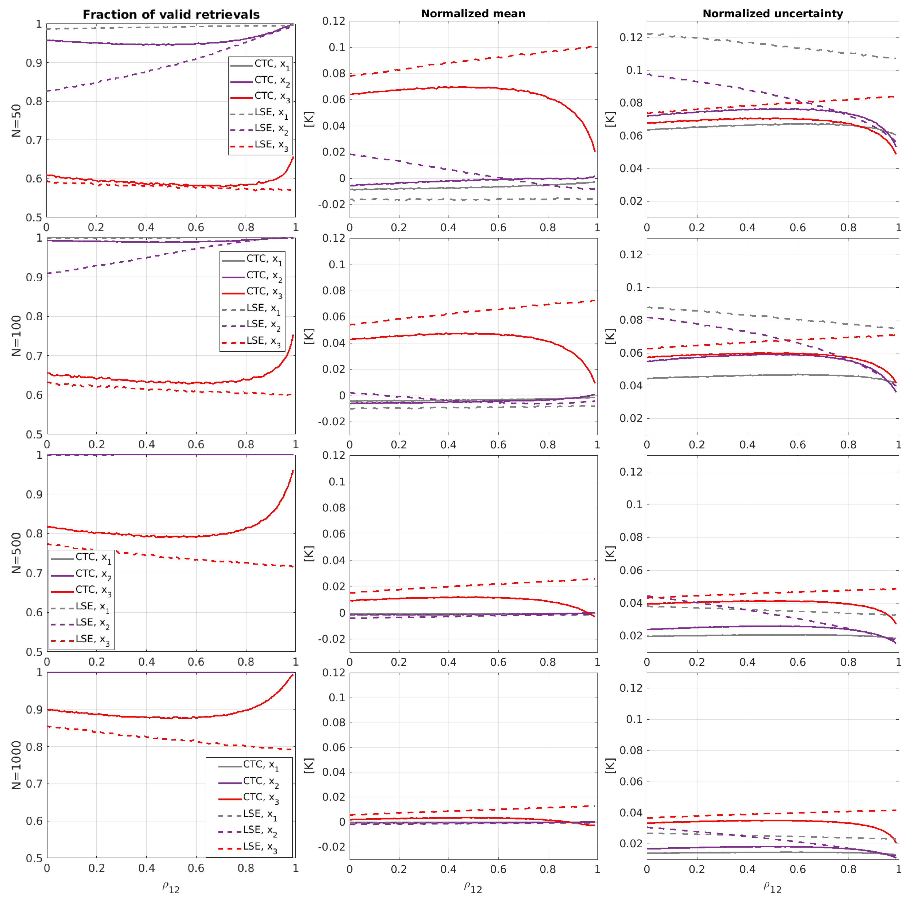
Figure 1. Quality assessment for test case 1 (“small uncorrelated”) ( σ δ 1 = 0.5 , σ δ 2 = 0.25 , and σ δ 3 = 0.1 ): the results are shown as a function of the correlation parameter ρ 12 . From left to right: Fraction of valid retrievals, normalized mean, and normalized uncertainty. From top to bottom: Results for N = 50 , N = 100 , N = 500 , and N = 1000 . Grey color corresponds to the measurement x 1 , purple is for measurement x 2 , and red is for measurement x 3 . Solid lines are the results for correlated triple collocation, while dashed lines are for least squared error triple collocation.
Remotesensing 12 03381 g001
Figure 2. Quality assessment for test case 2 (“equal”) ( σ δ 1 = 0.5 , σ δ 2 = 0.5 , and σ δ 3 = 0.5 ): the results are shown as a function of the correlation parameter ρ 12 . From left to right: Fraction of valid retrievals, normalized mean, and normalized uncertainty. From top to bottom: Results for N = 50 , N = 100 , N = 500 , and N = 1000 . Grey color corresponds to the measurement x 1 , purple is for measurement x 2 , and red is for measurement x 3 . Solid lines are the results for correlated triple collocation, while dashed lines are for least squared error triple collocation.
Remotesensing 12 03381 g002
Figure 3. Quality assessment for test case 3 (“large uncorrelated”) ( σ δ 1 = 0.1 , σ δ 2 = 0.25 , and σ δ 3 = 0.5 ): the results are shown as a function of the correlation parameter ρ 12 . From left to right: Fraction of valid retrievals, normalized mean, and normalized uncertainty. From top to bottom: Results for N = 50 , N = 100 , N = 500 , and N = 1000 . Grey color corresponds to the measurement x 1 , purple is for measurement x 2 , and red is for measurement x 3 . Solid lines are the results for correlated triple collocation, while dashed lines are for least squared error triple collocation.
Remotesensing 12 03381 g003
Figure 4. Log-log plot of the standard deviation of the intercalibration factors as a function of the sampling size N: purple represents the standard deviation of α 12 , and green represents the standard deviation of α 13 . (a) The results for case 1, (b) the results for case 2, and (c) the results for case 3.
Remotesensing 12 03381 g004
Figure 5. Assessment of the impact of varying the intercalibration factor α 13 on the estimates provided by Correlated Triple Collocation (CTC). Top: Number of valid retrievals per measurement as a function of the α 13 value (measurements 1, 2, and 3 are attributed to the colors grey, purple, and red, respectively). Bottom: Biases on the retrieved error standard deviations as a function of α 13 . The columns from left to right are for the “small uncorrelated”, “equal”, and "large uncorrelated" cases defined in Section 2.2.
Remotesensing 12 03381 g005
Figure 6. Log-log plots of the Power Density Spectra (PDS) of the three datasets: green represents Soil Moisture and Ocean Salinity (SMOS) nominal, blue represents SMOS nodal sampling (NS), and purple represents Soil Moisture Active Passive (SMAP). (a) Central Asia and (b) Central Africa.
Remotesensing 12 03381 g006
Figure 7. (a) Map of the intercalibration factor between SMOS nominal and SMOS NS ( α 12 ), (b) map of the intercalibration factor between SMOS NS and SMAP ( α 13 ), (c) histogram of α 12 , and (d) histogram of α 13 .
Remotesensing 12 03381 g007
Figure 8. Map of the error correlation ( ρ 12 ) between SMOS nominal and SMOS NS (mean correlation: 0.71 and data gaps: 5.23 % ).
Remotesensing 12 03381 g008
Figure 9. SMOS Radio Frequency Interference (RFI) probability map in the period 1 January 2016 and 30 June 2017 computed following the procedure detailed in [37].
Remotesensing 12 03381 g009
Figure 10. Maps of the error standard deviation of brightness temperature (TB) ( σ δ i ): (a) SMOS nominal (mean error std: 7.23 K and gaps: 1.02%), (b) SMOS NS (mean error std: 6.2 K and gaps: 1.34%), and (c) SMAP (mean error std: 3.18 K and gaps: 14.88%).
Remotesensing 12 03381 g010
Figure 11. Zoom in of the error standard deviation maps shown in Figure 10: (a,c) SMOS nominal and (b,d) SMOS NS. Note the change of scale with respect to the one used in Figure 10.
Remotesensing 12 03381 g011
Figure 12. Maps of the difference between the error standard deviation of TB (a) SMOS nominal-SMOS NS (mean difference: 1.03 K), (b) SMOS nominal-SMAP (mean difference: 3.41 K), and (c) SMOS NS-SMAP (mean difference: 2.28 K).
Remotesensing 12 03381 g012
Figure 13. Histograms of the difference between the error standard deviation of SMOS nominal and SMOS NS: (a) global map and (b) RFI-contaminated region. Those points with error standard deviations higher than 15 K in absolute value are accounted for in the red bars.
Remotesensing 12 03381 g013
Figure 14. (a) Standard deviation of the SMAP measurements ( σ 3 ) for the analyzed period (June 2016–September 2017) NS (b) SMAP error standard deviation conditioned to SMAP TB standard deviation.
Remotesensing 12 03381 g014
Figure 15. Maps of the adjusted error standard deviation of TB ( σ δ i ) over land: (a) SMOS nominal (mean error std: 7.62 K and gaps: 0.05%,), (b) SMOS NS (mean error std: 6.62 K and gaps: 0.29%), and (c) SMAP (mean error std: 3.2 K and no gaps per construction).
Remotesensing 12 03381 g015aRemotesensing 12 03381 g015b
Figure 16. Map of the difference between the error standard deviation of SMOS nominal and SMOS NS TBs (mean reduction of the error standard deviation led by NS: 0.99 K).
Remotesensing 12 03381 g016
Figure 17. Histogram of the difference between error standard deviation of nominal TB and error standard deviation of NS TB after the adjustment detailed in this section (mean error std: 1 K): those points with error standard deviations higher than 15 K in absolute value are accounted for in the red bars (excess bars). (a) Global; (b) RFI region.
Remotesensing 12 03381 g017
Publisher’s Note: MDPI stays neutral with regard to jurisdictional claims in published maps and institutional affiliations.