We carry out a series of experiments on simulated and real data and compare our proposed method with the Lee filter, Goldstein filter, and InSAR-BM3D filter under the same experimental conditions in order to verify the effectiveness and robustness of the proposed method. For a clear comparison, qualitative and quantitative indexes are used for performance evaluation. All of the experiments were implemented on a PC with an i9-9900k CPU and an NVIDIA GeForce GTX 2080Ti GPU, and our proposed method is implemented on TensorFlow platform based on Python 3.6.6.
4.1. Experiments on Simulated Data
The data set was generated while using the simulated method that is described in
Section 3.1. The size of the initial Gaussian distributed random matrix, the range of the unwrapped phase and the level of added noise are set to
, 0–20 rad and −1.49 dB, respectively. The training set contains 10,000 pairs of real part images and 10,000 pairs of imaginary part images, and the testing set contains additional 2500 pairs of real part images and 2500 imaginary part images. We use Adam optimizer with a mini-batch size of 10 [
41] and Glorot’s method [
50] to initialized all trainable variables. The learning rate is exponentially decayed from an initial value of 1
to 0 with a power of 0.3. Early Stopping [
51,
52] is used to choose when to stop iteration, and 120,000 iterations are enough for convergence in our experiment that takes about six hours. In each iteration, the input training samples are randomly selected. After training, the trained PFNet was tested by the testing samples. We first randomly select a testing sample in order to visually analyze the filtering performance and then calculate the average evaluation indexes of all testing samples for quantitative analysis.
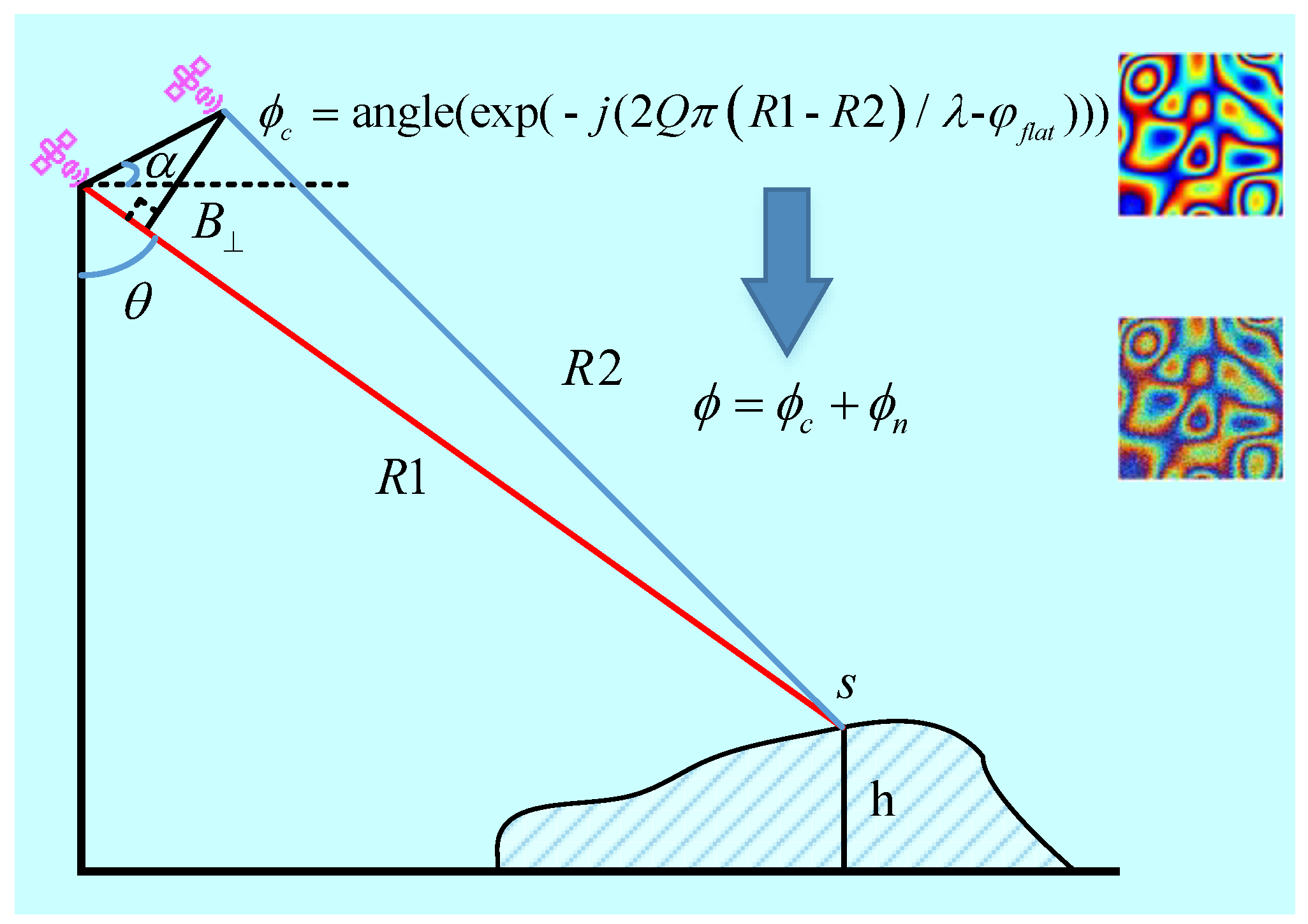
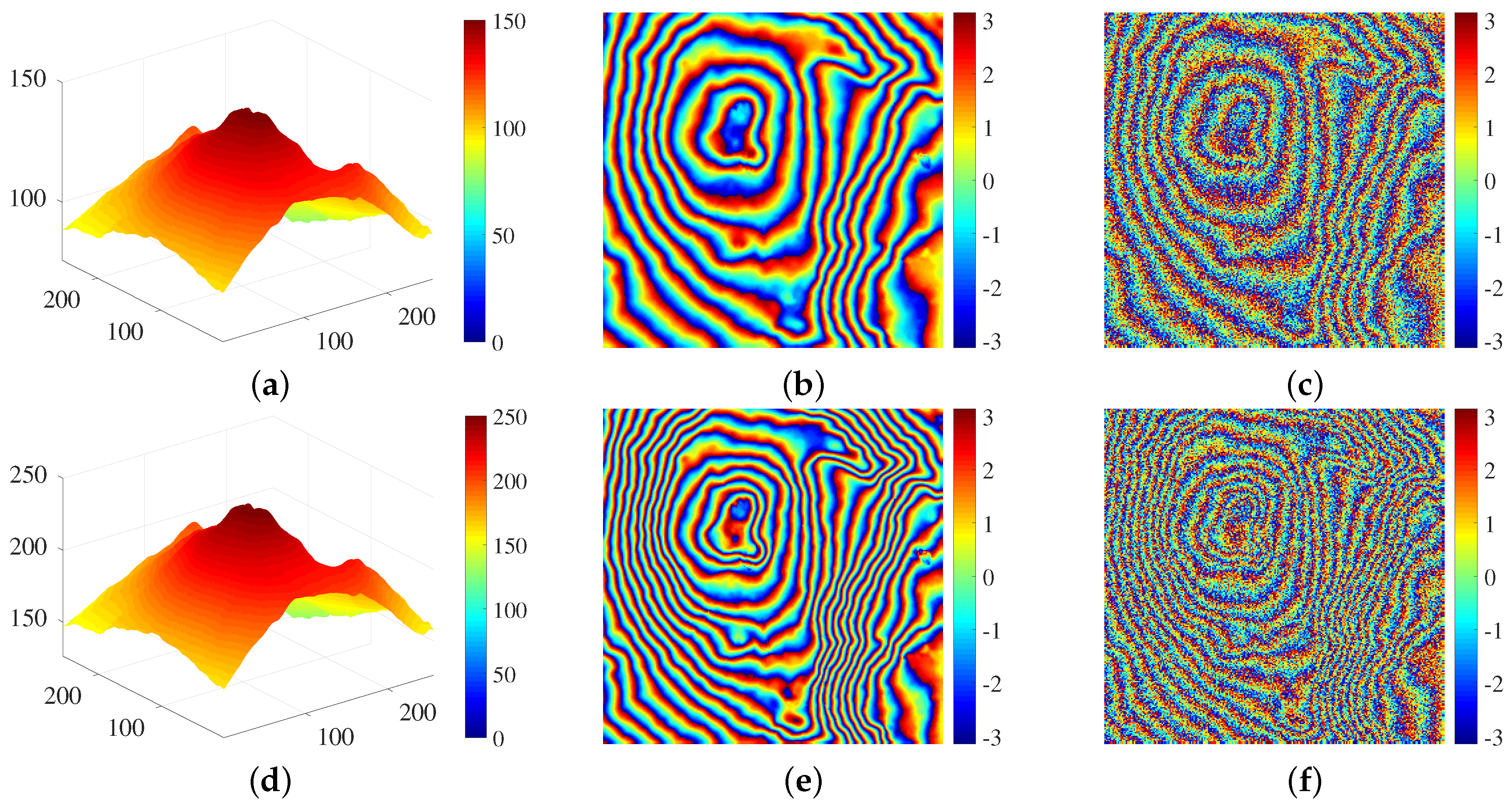
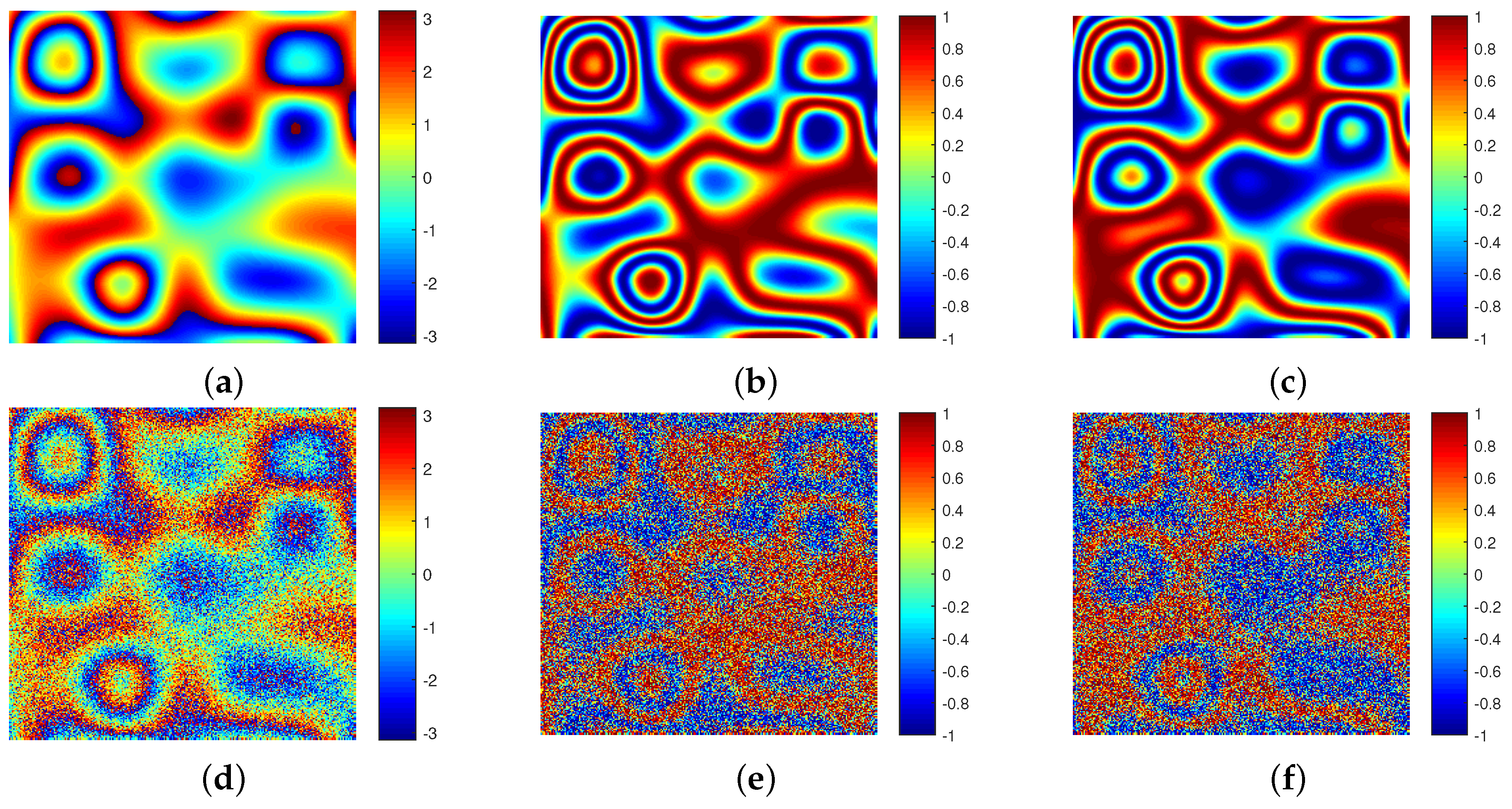
A clean interferometric phase image and its real part and imaginary part images are shown in
Figure 9a–c, respectively. After noise is added, the corresponding noisy interferometric phase image and its real part and imaginary part images are shown in
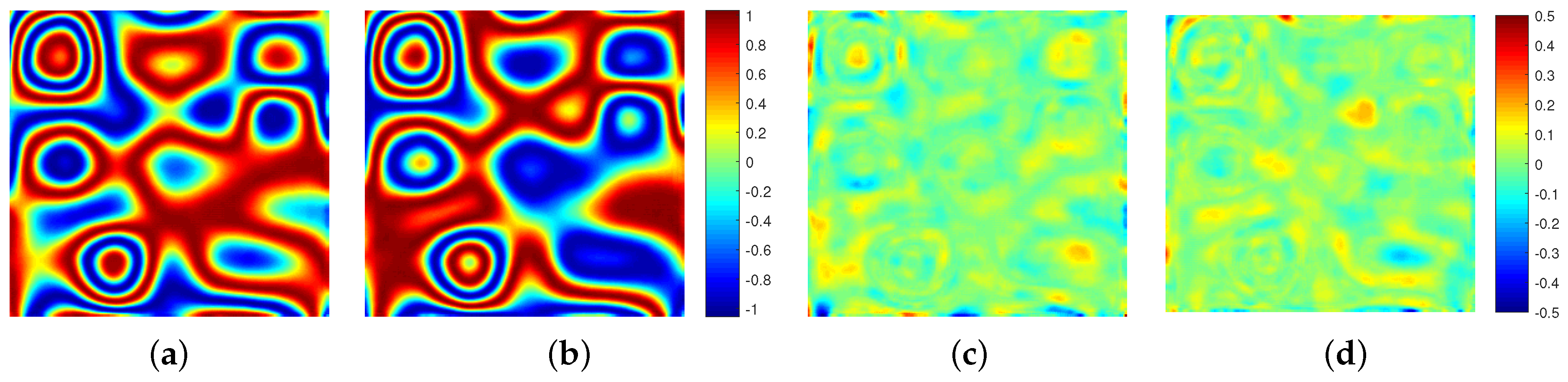
Figure 9d–f, respectively. The noisy real part and imaginary part images are filtered using the trained PFNet, and the filtered versions and the phase differences between the filtered version and the clean version are shown in
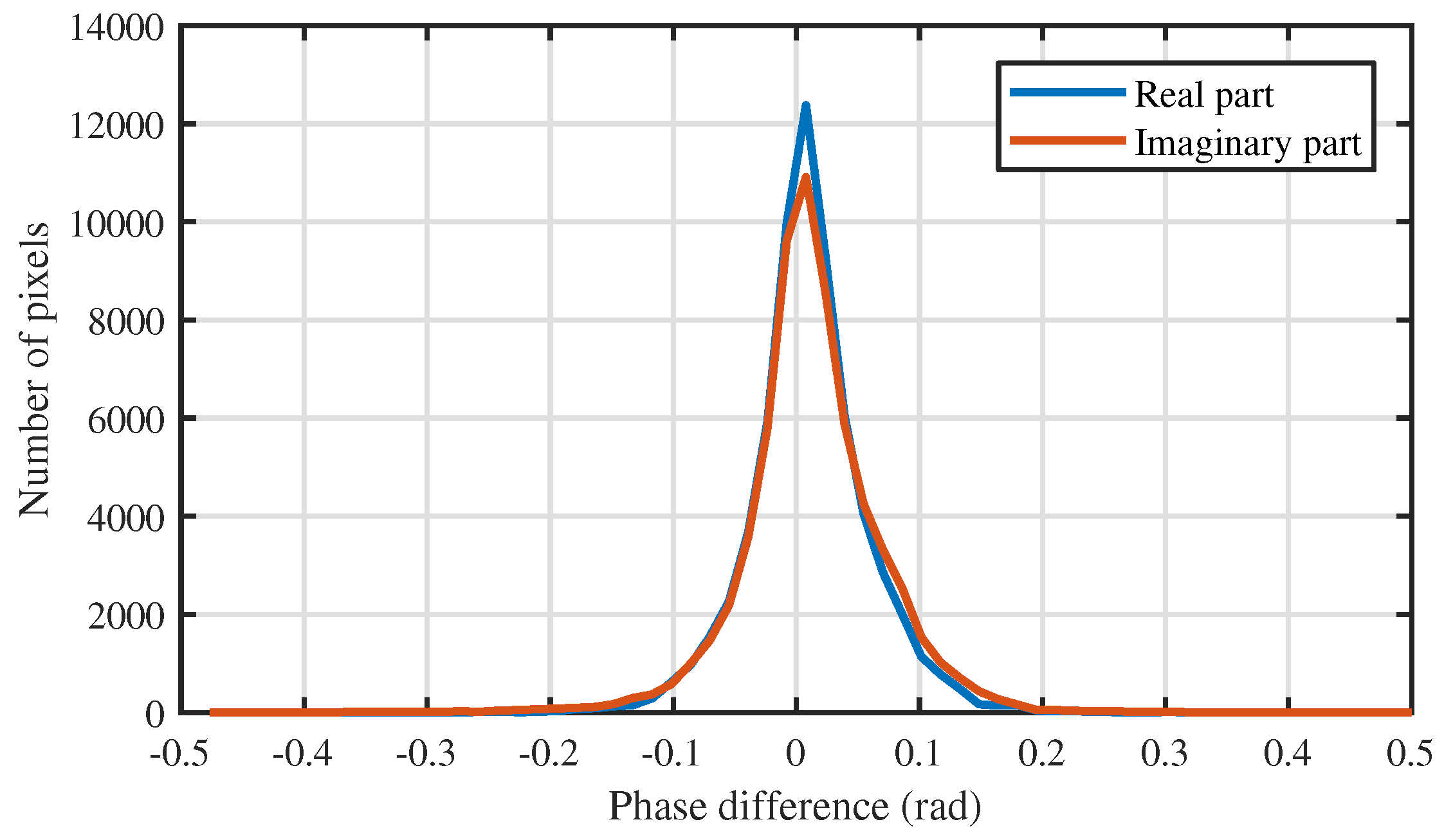
Figure 10. We can observe that the filtered real part and imaginary part images are very close to the corresponding clean real part and imaginary part images, because most of the pixels of the phase difference images are close to zero. In order to more intuitively and clearly show this phase difference, the fitted histogram curves of the phase differences are shown in
Figure 11. The histogram curve is plotted according to the value of the phase difference histogram, which reflects the distribution density of the phase difference. The vertical axis is the number of pixels and the horizontal axis is the value of the phase difference. From
Figure 11, it can be seen that the two curves are sharp near zero, which indicates that the differences are small and concentrated near zero, that is, the noise is well suppressed in the real and imaginary parts of the noisy interferometric phase. According to the filtered real and imaginary parts, the filtered interferometric phase can be obtained using Equation (
6).
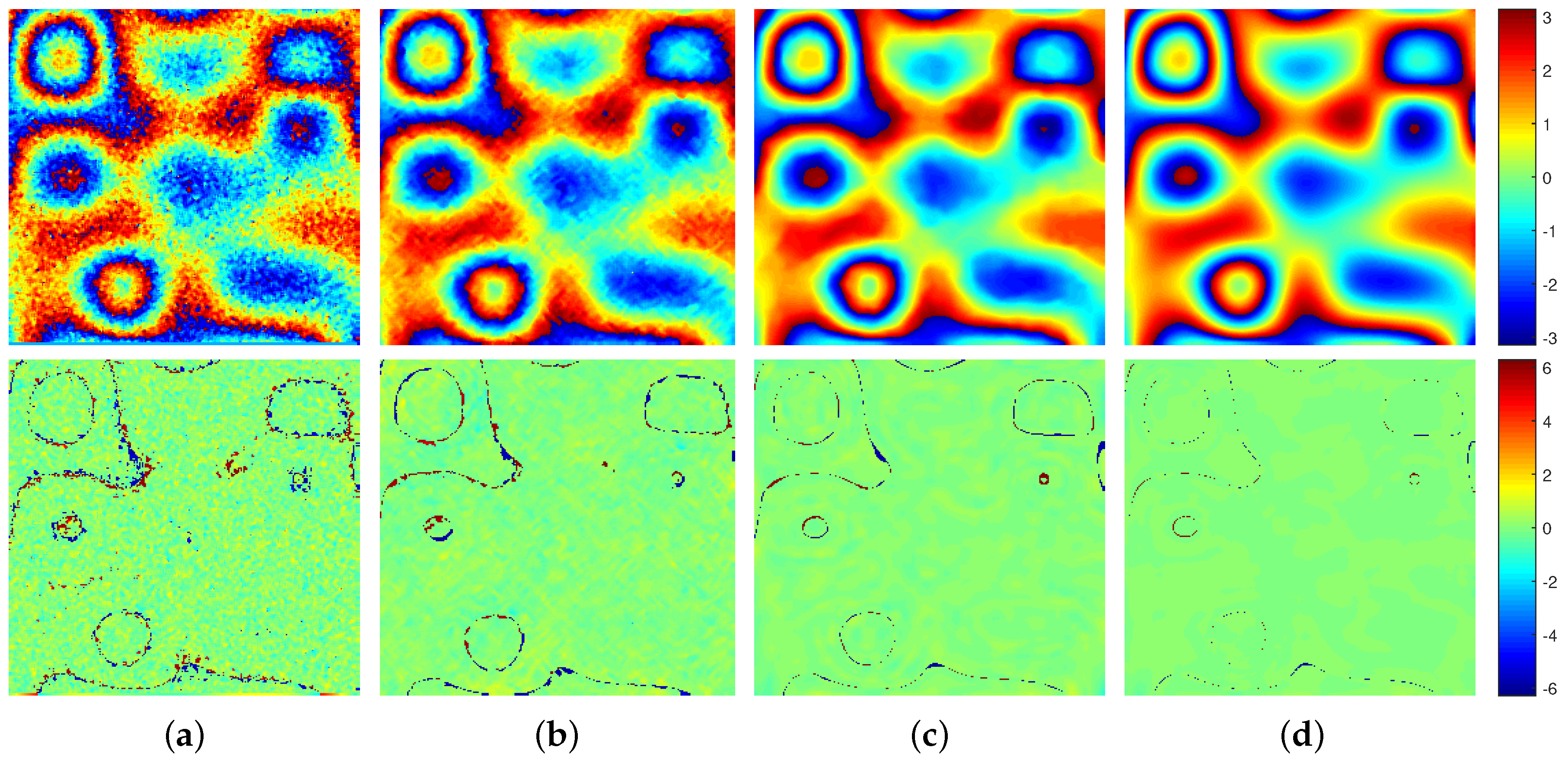
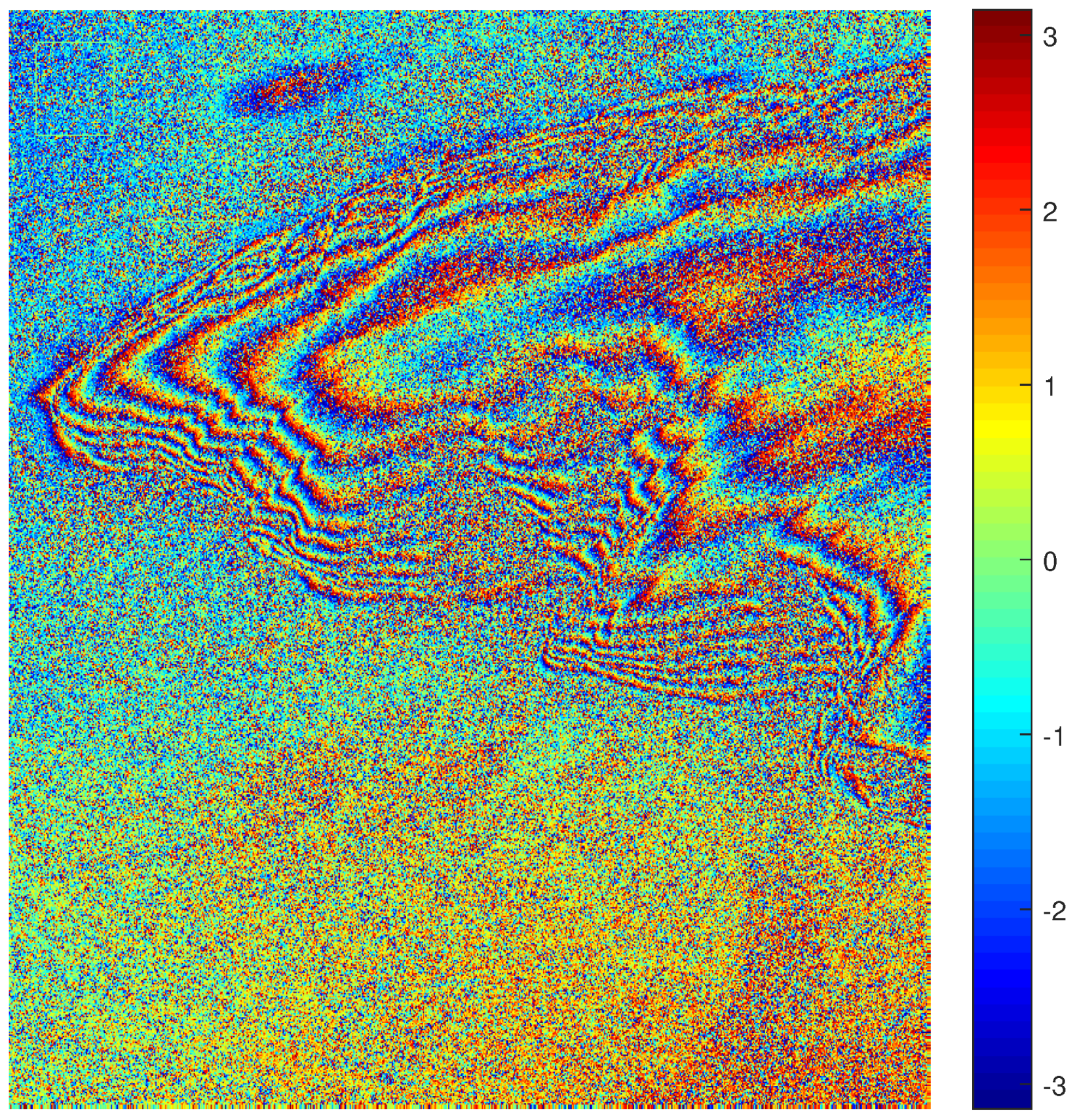
We compare our proposed method with three widely-used methods in order to further analyze the performance of the proposed method: the Lee filter, Goldstein filter, and InSAR-BM3D filter.
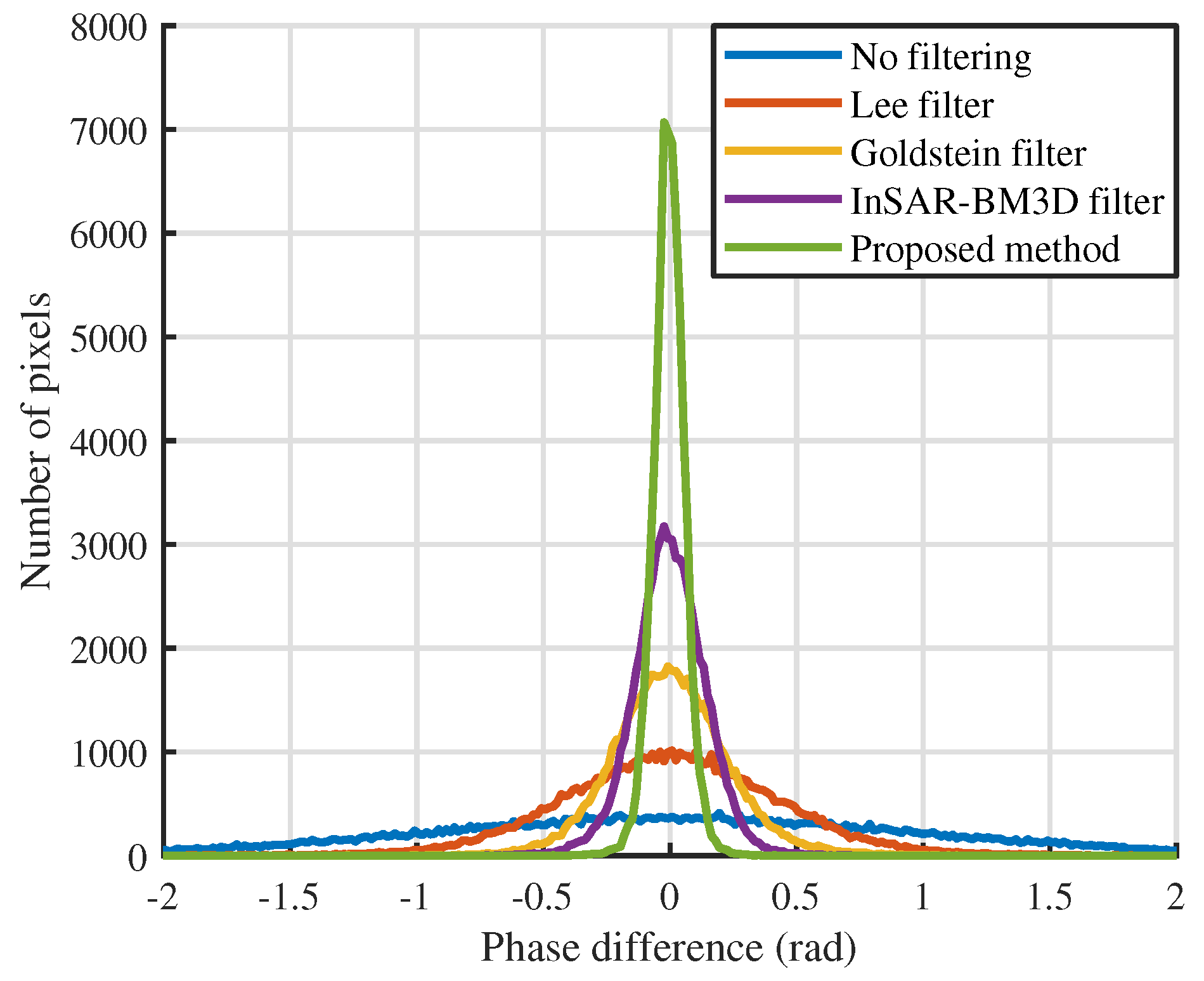
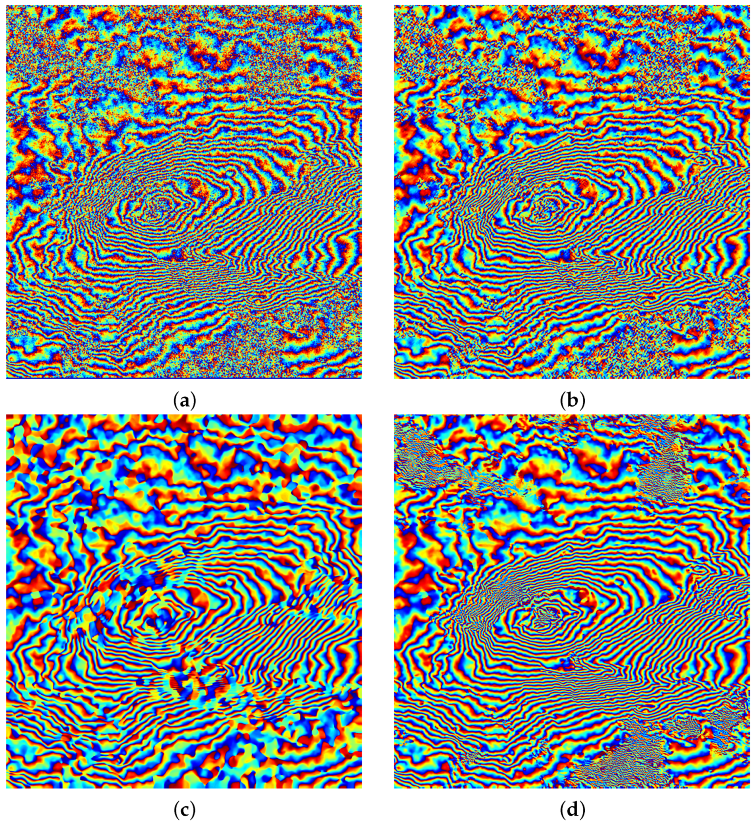
Figure 12 shows the filtered interferometric phase images and the phase difference between the clean phase and filtered phase. We can see that the result of the proposed method is very close to the clean interferometric phase and is better than the other three methods from the naked eye, because its phase difference image is closer to zero. In order to more intuitively and clearly show this phase difference, the fitted histogram curves of the phase differences are shown in
Figure 13. We can see that the fitted curve of the proposed method is sharper near zero than that of other methods, which indicates that the phase difference of the proposed method is more centered on zero, that is, the proposed method is significantly better from the perspective of the phase difference. Furthermore, the four aforementioned evaluation indexes, namely NOR, MSSIM, MSE, and
T, are adopted and listed in
Table 2. We can see that the proposed method obtains the lowest NOR and MSE, and the highest MSSIM, which reveals that the proposed method filters out the most noise and maintains the most detailed information among the four methods, which is, the proposed method has the strongest noise suppression capacity and the detail preservation capacity. In more detail, when compared with the InSAR-BM3D filter, the MSSIM and MSE of the proposed method are improved by 19.62% and 51.15%. Meanwhile, the proposed method has the smallest runtime (
T), which means that it has a great advantage in computational efficiency. From another perspective, the proposed method has the highest accuracy, because the comprehensive evaluation of MSSIM and MSE reflects the accuracy of phase filtering. Combining accuracy and computational efficiency to analyze, we note that, although the runtime of the Lee filter and the Goldstein filter are less than the InSAR-BM3D filter, their MSSIM and MSE is not as good as the InSAR-BM3D filter. This contradiction between accuracy and computational efficiency has been resolved in the proposed method, because the runtime of the proposed method is the smallest and its accuracy is highest among the four methods. In summary, the proposed method is superior to the other three methods from qualitative and quantitative perspectives.
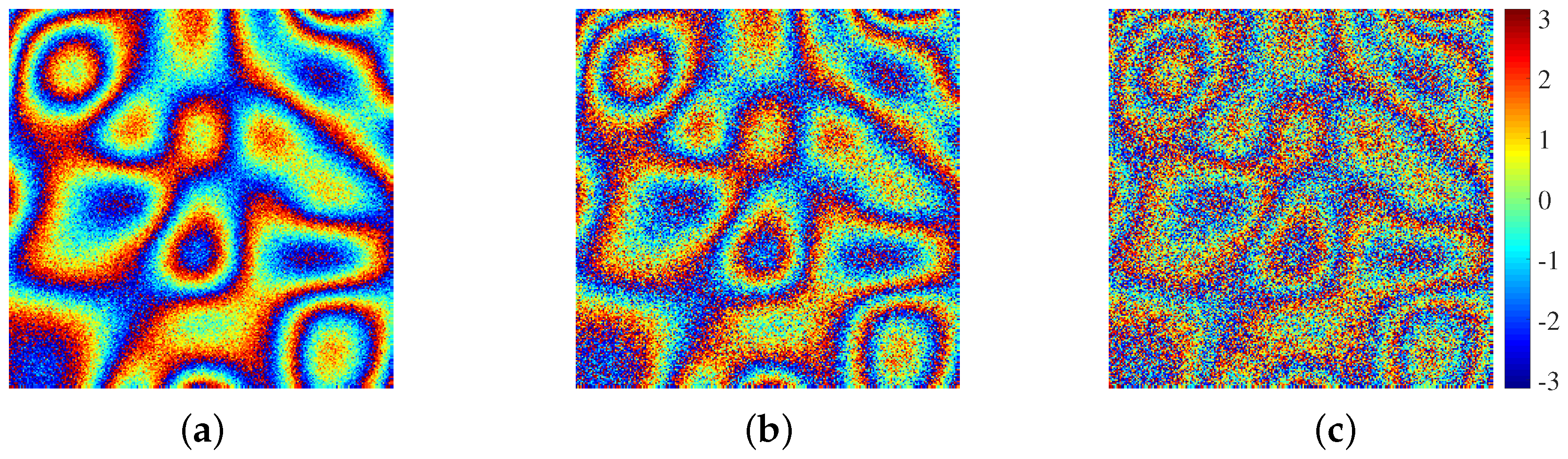
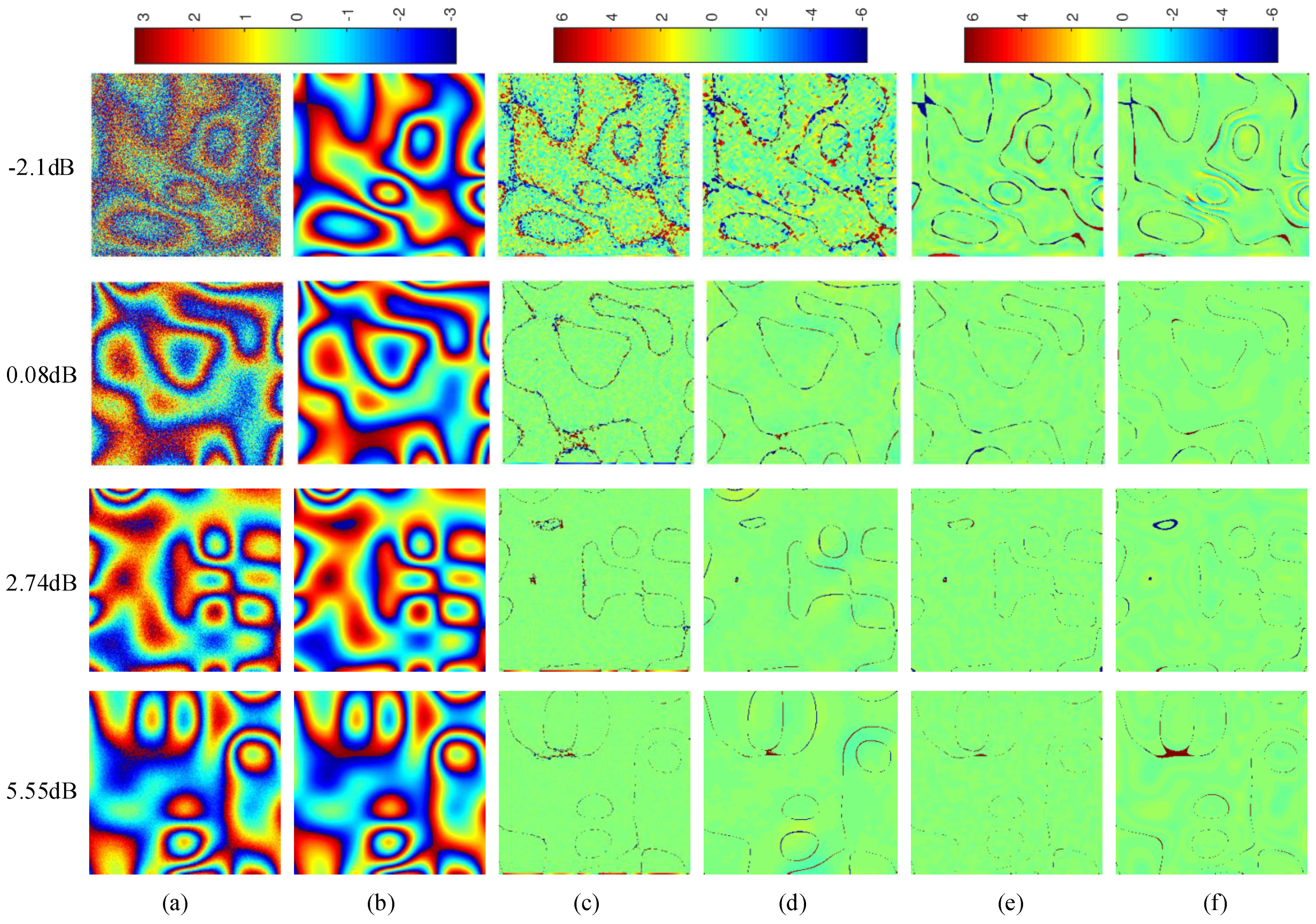
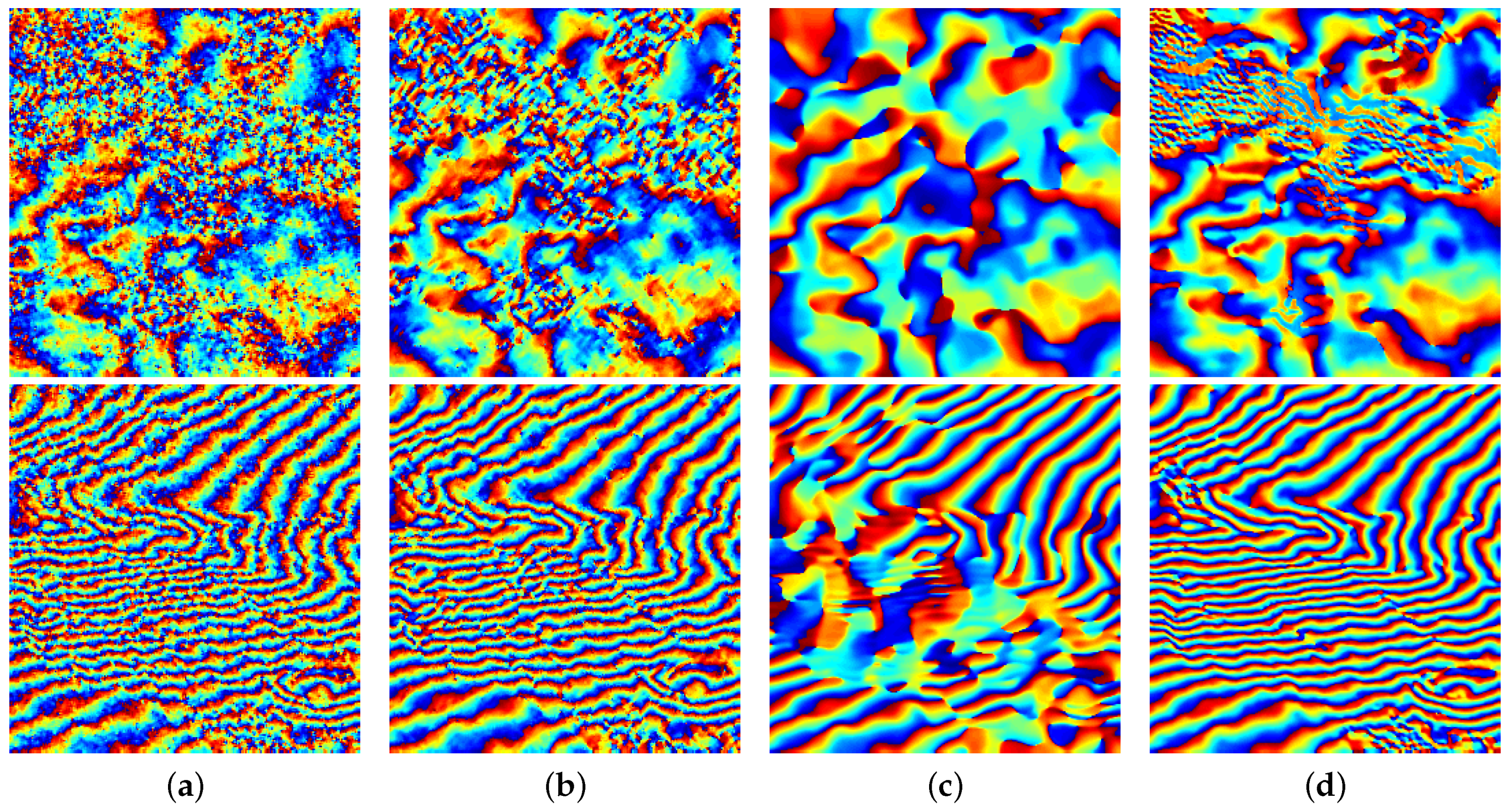
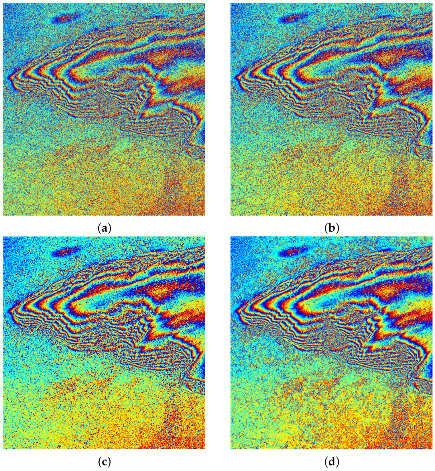
In the above experiments, the SNR of all testing samples is the same as the training samples, but, in practical applications, the SNR of the testing sample may be different from the training sample. Therefore, we next analyze the robustness of the proposed method when processing images with different values of SNR. We select four situations covering the range of noise from strong to weak for visual display, and the filtered results of four methods are shown in
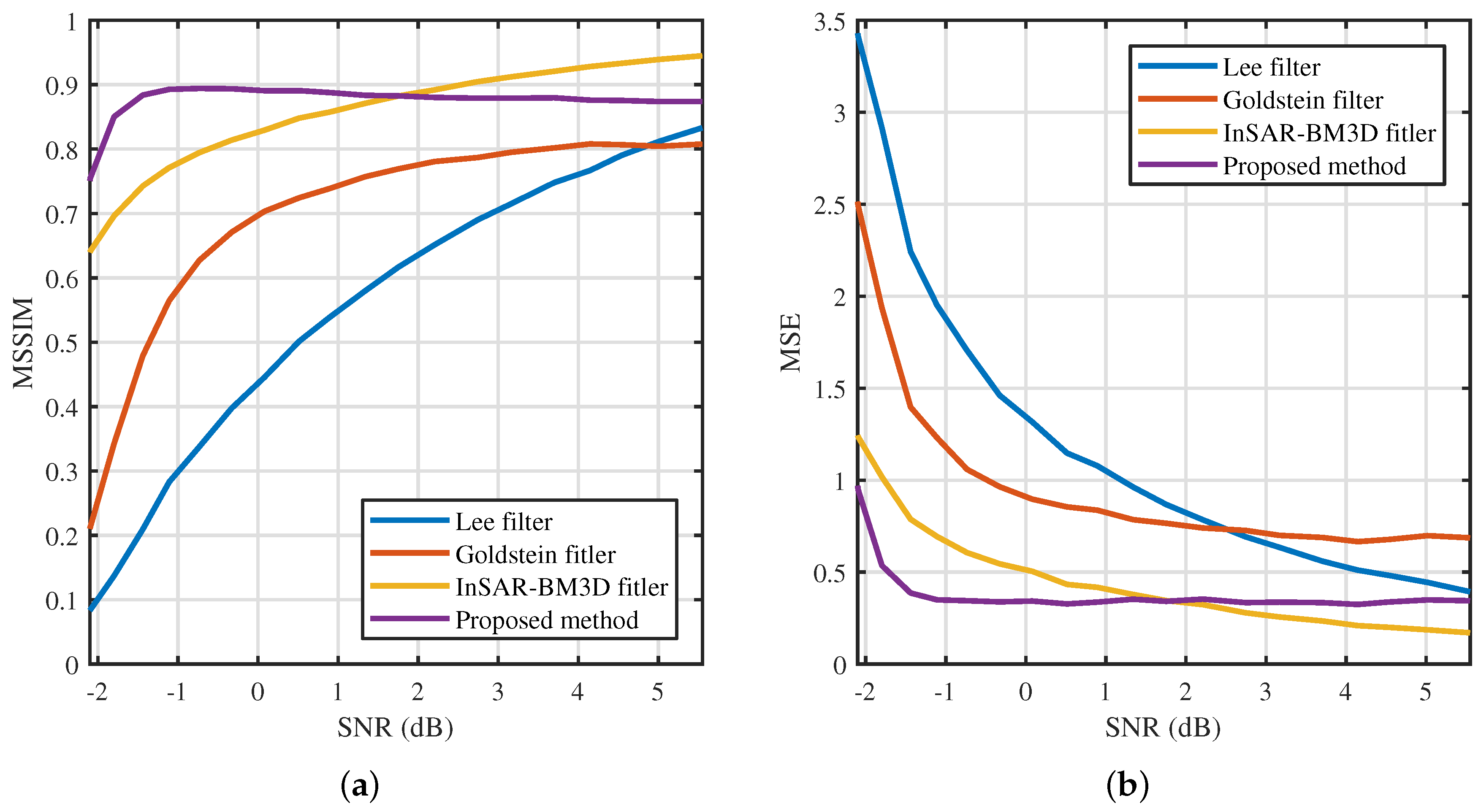
Figure 14. It can be seen that the proposed method and InSAR-BM3D filter outperform the other two methods in these four cases because their phase difference is closer to zero. Furthermore, when the SNR (−2.1 dB, 0.08 dB) of the testing sample is close to that of the training sample (−1.49 dB), the proposed method outperforms the InSAR-BM3D filter, and when the SNR (2.74 dB, 5.55 dB) of the testing sample is far from that of the training sample, the performance of the InSAR-BM3D filter is better than the proposed method. In order to quantitatively analyze the above-mentioned inferences, we calculated the MSSIM and MSE of each method according to the filtered results in the SNR range of (−2.1, 5.55) dB, as shown in
Figure 15. It can be seen that the MSSIM of the proposed method and the InSAR-BM3D filter is significantly higher than the other two methods, and their MSE is significantly lower than the other two methods, which indicates that the capacities of noise suppression and detail preservation of the proposed method and InSAR-BM3D filter are significantly better. Next, comparing the proposed method with the InSAR-BM3D filter, the proposed method is significantly better than the InSAR-BM3D filter when the SNR of the testing sample is close to that of the training sample, which reveals that as long as the SNR of the testing sample keeps within a certain interval with the that of the training sample, the proposed method can obtain better performance than the InSAR-BM3D filter. Moreover, it is worth noting that the difficulty of filtering is greatly reduced in the case of high SNR, and the performance of the filtering algorithm in the case of low SNR is more worthy of attention. This is also the reason for choosing a lower SNR of training samples.
We carry out four experiments under the same condition, and each experiment halves the number of training samples in order to test the impact of the sample reduction on the performance of the proposed method. Their MSSIM and MSE are calculated and listed in
Table 3. From
Table 2 and
Table 3, we can find that as the number of training samples decreases, the performance of the proposed method decreases slightly, but it is still better than the other three methods. That is to say, the performance of the proposed method is still better than the other three methods when the number of training samples is reduced by eight times.
In order to further demonstrate the performance of the proposed method, we compare it with another deep learning filtering method (called DeepInSAR) [
35]. For a fair comparison, the data set used in this paper is the same as the data set used in [
35] in terms of the data simulation method and number of images. The code of the simulation method can be downloaded from
https://github.com/Lucklyric/InSAR-Simulator. The training set contains 28,800 pairs of real part images of simulated interferometric phases and 28,800 pairs of imaginary part images of simulated interferometric phases with a size of
, and the testing set contains additional 900 pairs of simulated real part images and 900 pairs of simulated imaginary part images with a size of
. In this experiment, the proposed method converges after 345,600 iterations, and the filtered results are obtained by the testing process. For quantitative analysis, the MSSIM and Root Mean Square Error (RMSE) of DeepInSAR are taken from [
35], and the indexes of the two methods are listed in
Table 4. From
Table 4, it can been seen that the MSSIM of the proposed method is comparable to DeepInSAR, and its RMSE is greatly improved by 21.47%. Therefore, the overall performance the proposed method is better than DeepInSAR on the same data set.


