Abstract
In this study, the performance and characteristics of the advanced cloud nucleation scheme of Fountoukis and Nenes, embedded in the fully coupled Weather Research and Forecasting/Chemistry (WRF/Chem) model, are investigated. Furthermore, the impact of dust particles on the distribution of the cloud condensation nuclei (CCN) and the way they modify the pattern of the precipitation are also examined. For the simulation of dust particle concentration, the Georgia Tech Goddard Global Ozone Chemistry Aerosol Radiation and Transport of Air Force Weather Agency (GOCART-AFWA) is used as it includes components for the representation of dust emission and transport. The aerosol activation parameterization scheme of Fountoukis and Nenes has been implemented in the six-class WRF double-moment (WDM6) microphysics scheme, which treats the CCN distribution as a prognostic variable, but does not take into account the concentration of dust aerosols. Additionally, the presence of dust particles that may facilitate the activation of CCN into cloud or rain droplets has also been incorporated in the cumulus scheme of Grell and Freitas. The embedded scheme is assessed through a case study of significant dust advection over the Western Mediterranean, characterized by severe rainfall. Inclusion of CCN based on prognostic dust particles leads to the suppression of precipitation over hazy areas. On the contrary, precipitation is enhanced over areas away from the dust event. The new prognostic CCN distribution improves in general the forecasting skill of the model as bias scores, the root mean square error (RMSE), false alarm ratio (FAR) and frequencies of missed forecasts (FOM) are limited when modelled data are compared against satellite, LIDAR and aircraft observations.
1. Introduction
Dust particles cover approximately 50% of the global load of the natural airborne particles [1,2]. Dust aerosols interact with electromagnetic radiation [3] and directly affect the radiation budget of the land–atmosphere system (aerosol direct effect) [4]. Furthermore, they absorb and scatter in various wave lengths both solar and long wave radiation [5,6,7,8]. Consequently, they modify the heating rates, the stability and the stratification of the atmosphere [9,10]. Additionally, dust interactions with radiation influence both the Asian [11] and the African monsoonal circulations [12,13]. Moreover, dust particles have an important impact on human health [14,15,16,17,18] and alter the biochemical cycles of both land and sea ecosystems [19].
Furthermore, the concentration and the characteristics of the dust particles have a strong impact on cloud formation and the hydrological cycle in general, as dust acts as effective cloud condensation (CCN) and ice nuclei (IN), respectively [20,21,22,23,24]. The increase in the active CCN number due to the high levels of dust aerosols in the atmosphere leads to cloud formations with droplets of higher concentrations but with smaller diameters. This is the first indirect effect of the dust aerosols to cloud formations, which increases the cloud albedo [25,26]. The increase in CCN particles may also lead to precipitation suppression [27], enhancement of the cloud height [28] and an increase in the lifetime of the clouds [21]. These mechanisms are considered as the second indirect effect. Moreover, the solar energy absorbed by dust particles leads to the increase in the atmospheric temperature of the surrounding layers, which decreases cloudiness [29] and is often called the semi-direct effect.
As it is also stated above, according to the “Twomey” effect [25], an increased number of CCN affects the precipitation mechanisms, as it produces more cloud drops with smaller diameters (hazy cloud formation). An increased droplet number also leads to an enhanced cloud reflectance with constant amounts of liquid water. However, in this case, the transformation time of cloud to rain droplets increases. Thus, the precipitation mechanisms are limited during the early stages of the cloud formations in comparison to pristine clouds (clouds with low levels of particles). On the other hand, the latent heat released by condensation in the lower cloud levels supports severe upward motions and enhances the vertical mixing [30]. Furthermore, the precipitation delay may cause significant droplet advection to the middle and upper level of the clouds. Hence, under specific atmospheric conditions, hazy clouds are able to enhance the precipitation patterns over locations away from the cloud formation areas and with a time delay of many hours [31,32,33]. Thus, in a thunderstorm, the precipitation may be delayed at the initial thunderstorm stage due to the increased CCN concentration. However, the initial thunderstorm may convert to an autonomous squall line due to the interactions between the cool pools and the wind shear. Other modelling studies propose that this thermodynamic enhancement is insignificant or limited, especially for cold-based clouds in dry conditions of important wind shear [34,35]. On the contrary, observational studies claim that a hazy atmosphere contributes to an enhanced cloud cover with an increased height of cloud ceiling [36,37,38]. Thus, cloud convection is enhanced, as fall-velocity and ice particles reduce.
Despite the fact that many studies have examined the role of airborne particles as active CCN or IN, there are still uncertainties concerning their impact on cloud formations and the precipitation pattern [5,39,40]. Furthermore, it is not quite clear yet how the aerosols’ concentrations, sizes and chemical compositions may influence the aerosol–cloud interaction processes. Additionally, the impact of aerosols on radiation alters the dynamical and thermodynamical structure of the atmosphere. However, it has to be examined when this impact enhances or decreases the precipitation [12,41,42]. These phenomena affect, importantly, the time triggering of precipitation and the characteristics of a thunderstorm [32,33,43,44].
Various studies support that an increase in the aerosol levels leads to the suppression of precipitation that originates from large-scale stratiform clouds [45,46], following the “Twomey effect” stated above. However, the aerosol impact on precipitation from deep convective clouds is still an unresolved issue [47,48,49]. Some studies show that an increase in the aerosol levels suppresses the precipitation during severe rainfall cases [50], while others support that precipitation is enhanced as the CCN concentration rises at a specific level [51]. Furthermore, it is widely acceptable that, under conditions of high humidity (mostly tropical convection), deep convective clouds are strengthened, while the precipitation of small clouds is suppressed [47,48,49]. In the study of Grell and Freitas [52], aerosol feedbacks have been added in convective cloud parameterizations, based on the conversion of cloud water into rain depending on CCN levels. Moreover, Berg et al. [53] embedded parameterizations of cloud effects on aerosols and gases into the Kain–Fritsch cumulus scheme. However, the above authors did not consider these treatments in terms of microphysics [54].
The main aim of this modeling study is to investigate the dust aerosols indirect effects on cloud formation and precipitation during a Saharan dust outbreak over the Western Mediterranean and Europe accompanied by torrential rainfall. The dynamical impacts of dust aerosols acting as effective CCN have been assessed through the implementation of the advanced cloud nucleation scheme of Fountoukis and Nenes [55]. This scheme is incorporated in a double-moment cloud microphysics scheme of the Weather Research and Forecasting/Chemistry (WRF/Chem) model [56,57]. WRF incorporates a variety of single [58,59,60,61] and double-moment [13,62,63,64,65,66] cloud microphysics schemes. Among the numerous double-moment schemes, the six-class WRF Double-Moment (WDM6) [13,67] is chosen as it also calculates the CCN concentration number and thus it is suitable for a direct evaluation of CCN concentration with observational data. WDM6 is an evolution of WRF’s six-class Single-Moment (WSM6) [61] microphysics scheme, which has also included graupel as a prognostic variable. However, WDM6 does not take into account by default aerosols in order to calculate CCN concentrations. Instead, a constant CCN initial concentration is considered for the spatiotemporal CCN variability. Hence, the above deficiency has been overcome as the Fountoukis and Nenes [55] cloud nucleation scheme is embedded in the WDM6 scheme. However, some studies show that the choice of a cloud microphysics scheme is of little importance [68,69] and also investigate the importance of the cumulus parameterizations and convection, especially concerning the spatial “grey zones”. Thus, the cumulus parameterization scheme of the “scale aware” Grell and Freitas [52] has also been modified in order to take into account the simulated CCN concentrations by the Fountoukis and Nenes [55] cloud nucleation scheme.
2. Materials and Methods
2.1. The Embedded Cloud Nucleation Scheme
The WRF double-moment (WDM6) microphysics scheme [13] supports prognostic equations for water substance variables, such as cloud water, water vapor, rain, cloud ice, graupel and snow. Furthermore, it calculates the prognostic concentration number of CCN, cloud and rain water. The concentration number of ice species like graupel, snow and ice follows the diagnostic estimation of the ice phase process of Hong [70]. This simple estimation is theoretically accepted as the prediction of the ice phase number concentrations has less influence than the prediction of warm phase concentrations in deep convective cases [71]. Warm rain processes such as accretion and autoconversion are based on the methodology of Cohard [72]. The calculation of any other source/sink terms is based on the WRF single-moment (WSM6) microphysics scheme [61].
The prediction of the activated CCN concentration number uses the drop activation process based on the Twomey relationship, which links the activated CCN number and the supersaturation [20,73]. As the evaporation of cloud droplets is also considered, the corresponding CCN number is added to the total CCN concentration number. Any other sink/source mechanism apart from the CCN activation and evaporation is ignored. However, no real time CCN concentration is supported. Thus, a constant initial CCN number of 100 cm−3 [67] is used, in order to treat the CCN spatiotemporal distribution as a prognostic variable. The above value is representative of maritime aerosol particles, which can act as effective CCN [13]. The activated CCN number concentration is predicted using the drop activation by Twomey’s relationship between the number of activated CCN and supersaturation:
where nact is the activated CCN, n is the initial CCN value, Nc is the cloud droplet number concentration, S is the supersaturation and k (0.6 is set in the current study) is the parameter following the observation varying from 0.3 to 1.0 [73]. The evaporation of cloud droplets is also taken into account and returns CCN particles to the overall CCN count. Any other sink/source term is ignored. However, the above approximation remains the weakest link in this scheme, as there is no real time CCN replenishment [13].
The microphysics processes of WDM6 differ significantly from those of WSM6 due to the predicted concentration number of CCN, cloud (NC) and rain (NR) droplets. All microphysics processes are calculated according to the following cloud–rain drop distribution:
where indicates clouds or rain, νx and αx are the two dispersion parameters. NX and DX are the predicted total concentration number and diameter of the X drop category, respectively. The slope parameter λX is given by:
where vR = 2 and αR = 1 for rain and νc = 1 and αc = 3 for clouds. Moreover, qx (kg kg−1) is the mixing ratio for the X hydrometeor, ρα (kg m-3) and ρw = 103 (kg m−3) are the air and water density, respectively.
In this study, a prognostic initial number of CCN is applied, using the dust aerosol mass concentrations of the Georgia Tech Goddard Global Ozone Chemistry Aerosol Radiation and Transport of Air Force Weather Agency (GOCART/AFWA) emission scheme of the WRF/Chem model. The number concentration of dust particles N (kg−1) for an n size bin is calculated as:
where C is the dust mass mixing ratio (μg kg−1) for an m size bin. Summing up the N for all size bins (information concerning the bins is given in the following Section 3) gives the total concentration number of the dust aerosols.
The calculation of the prognostic initial concentration number of CCN is based on the parameterizations of the cloud droplet activation scheme of Fountoukis and Nenes [55], which is an evolution of the study of Nenes and Seinfeld [74]. This scheme (hereafter FN) represents the aerosol number and their chemical composition with respect to the size and the calculation of the initial CCN number (the CCN spectrum) at a specific supersaturation (s) level based on Köhler theory [75]. Furthermore, the CCN spectrum exists in the dynamical conditions of an air parcel with constant updraft velocity. The CCN spectrum Fs is given by:
where Ni is the aerosol number concentration, s is the supersaturation, sg,i the critical supersaturation, σi is the geographic standard deviation, i is the bin number. Processed dust is assumed to have the same hygroscopic properties as sulfate.
Moreover, the prognostic calculation of the cloud droplet concentration number is achieved through the computation of the maximum supersaturation (smax) as the air parcel ascends. With s = smax, the cloud droplet concentration number is given by:
The calculation of the smax is based on a parameterization of the water vapor balance. Full information on how the s, the sg,I and the smax are calculated can be found in the studies of Nenes and Seinfeld [74] and Fountoukis and Nenes [55]. It should be noted that CCN parameterizations of the original WDM6 scheme have not been deactivated in order to take into account the impact of sea salt particles.
As cumulus parameterization schemes are responsible for the simulation of convection, in this study, the CCN treatment by FN scheme has also been embedded in the Grell–Freitas (GF) cumulus parameterization scheme [52] in order to estimate the conversion rate and the precipitation efficiency on the CCN number concentration. The scheme includes modulation of convection by the environment (dynamic control), modulation of the environment by the convection (feedback) and a cloud model that defines the cloud properties (static control). Convection is triggered when the CAPE values are positive and the difference between cloud base (Lift Condensation Level LCL) and cloud top is 150 hPa minimum. Moreover, the LCL has to be within 50 hPa of the Level of Free Convection—LFC [76]. The original Grell and Freitas [52] cumulus scheme uses fixed values for CCN concentrations and for the conversion rate of condensation to precipitation. Thus, in this study, the prognostic CCN concentrations calculated by the implemented FN scheme are used. Furthermore, the above scheme is chosen as it is a scale aware scheme that can also be activated in the so-called “grey zones” concerning the spatial resolutions (6–10 km). Recent studies have shown that the activation of the GF scheme also in the so-called “grey zones” improves the overall precipitation pattern by reducing biases and improving root mean square error values [52,77].
2.2. Methodology
Τhe simulations are performed using the fully coupled meteorology–chemistry Weather Research and Forecasting/Chemistry model (version 3.9) WRF/Chem [56,57]. Both components use the same horizontal and vertical grids, the same physics schemes for the sub-grid scale transport and the same transport for the preserving of the air and scalar mass. Hence, the meteorological field is simultaneously simulated with the chemical field and the interactions in between. The chemical component is based on the Georgia Tech/Goddard Global Ozon Chemistry Aerosol Radiation and Transport (GOCART) module, which simulates tropospheric aerosols, such as sulfate, mineral dust, sea salt and black and organic carbon [78,79]. As far as the dust emissions are concerned, the Air Force Weather Agency (AFWA) package is used as it supports a non-experimental and sectional dust emissions scheme using an advanced set of dust emissions parametrizations [80,81], including five dust bins of 0.7, 1.4, 2.4, 4.8 and 8.0 μm effective radii. The scheme is based on a modified version of the saltation function of Marticorena and Bergametti [82]. The saltation for large-scale particles is triggered by wind shear and leads to fine particle emissions through bombardment [83]. There is a proportionality between horizontal and vertical dust flux, which is calculated when the friction velocity exceeds a specific threshold. The horizontal dust flux is calculated according to White [84]. The above proportionality is based on clay sand and erodibility fields. However, some studies [85] estimate that the linkage of the parametrized vertical dust flux to the clay fields is the main reason for the systematic overprediction of the simulated dust concentration. Furthermore, a correction to soil moisture parameterizations is applied [86]. The distribution of the emitted dust particles is based on the brittle fragmentation theory [87].
The GOCART/AFWA scheme supports by default a dust dry deposition scheme based on [88]. The calculation of dry deposition velocity is based on the aerodynamic, the quasi-laminar layer and the surface resistances. As far as wet deposition is concerned, the scheme of Seinfeld and Pandis [75] is implemented for both in and below cloud scavenging. It is shown in literature that especially the in-cloud area plays a leading role in the scavenging of suspended particles affecting the entire spatiotemporal distribution of the dust particles [89]. However, indirect effects concerning dust aerosols with cloud interactions are not supported. Hence, as is described in Section 2.1, the nucleation scheme of Fountoukis and Nenes [55] is embedded in the WDM6 [13,67] double-moment microphysics scheme. Furthermore, the fixed CCN concentrations used in the Grell–Freitas (GF) cumulus parameterization scheme [52] are replaced by the overall CCN concentrations calculated by the Fountoukis and Nenes [55] cloud nucleation scheme.
The performance of the Fountoukis and Nenes [55] scheme is assessed through a comparison of modelled precipitation against the WORLDVIEW-NASA satellite retrievals (Atmospheric Infrared Sounder–AIRS–Level 2). AIRS is an instrument based on the second Earth Observing System polar orbiting form (EOS–Aqua) and includes a group of infrared, visible and microwave sensors. The AIRS precipitation is an estimate of daily precipitation (in mm), with a 45 km spatial resolution with coverage twice a day. Parameters of cloud top pressure, fractional cloud cover and cloud-layer relative humidity have been used. Satellite data have been used as the amount of ground stations data for the specific areas were insufficient. The nearest model grid point values to the satellite ones have been used for the evaluation. A contingency table (Table 1) according to Wilks [90] methodology is used in order to calculate bias (B), false alarm ratio (FAR) and frequencies of missed forecasts (FOM). According to Table 1 a pairs mean that both observations and modeled values exceed a specific precipitation threshold. Similarly, b pairs mean that modelled values exceed the threshold but observation do not. Furthermore, c pairs mean that the model does not exceed the precipitation threshold; however, the observations are over it. Finally, d pairs mean that both model and observation did not manage to exceed the precipitation threshold

Table 1.
Contingency table following the Wilks [90] methodology.
B scores, FAR and FOM are calculated by:
Bias greater than one corresponds to the model’s overprediction, whereas bias less than one indicates the model’s underprediction. For unbiased forecasts, B is equal to one. For both FAR and FOM, best scores are equal to zero, whereas the value equal to one (or 100%) corresponds to the worst performance.
The response of the atmospheric optical properties to the explicitly resolved CCN patterns is further assessed through the use of LIDAR data of the EARLINET data base. The Aerosol extinction coefficient is used (550 nm–1.5 Level) instead of atmospheric optical depth (AOD), as the relationship between AOD and CCN is more complicated. More specifically, CCN concerning aerosol cloud interactions are located at the cloud area, whereas AOD is related to the entire atmospheric vertical column. Furthermore, the air mass may interact with clouds kilometers away or hours after the AOD measurements, which may occur under clear sky conditions [91]. Modelled CCN concentrations have also been compared against aircraft measurements (French aircraft service for environmental research-SAFIRE/MNPCA-CNRM/GAME) of ChArMEx/ADRIMED campaign (Chemistry-Aerosol Mediterranean Experiment/Aerosol Direct Radiative Impact on the regional climate in the MEDiterranean Region). The biases and the root mean square errors (RMSEs) concerning the above comparisons have been calculated by:
Moreover, a correlation coefficient (R) is calculated as a square root of Pearson correlation coefficient:
where Mi and Oi are the model estimates and the observed values respectively.
Configuration of the Modeling Experiments
In order to evaluate the performance of the embedded FN scheme in the WRF/Chem model, two experiments have been conducted, during a significant dust transport episode over the Western Mediterranean, characterized by torrential rainfall over Western Europe, during 19–25 June 2013. For this period and specific area, sulfate concentrations have been observed in the dust layer, during the ChArMEx/ADRIMED (the Chemistry-Aerosol Mediterranean Experiment/Aerosol Direct Radiative Impact on the regional climate in the MEDiterranean Region) campaign [92]. Aircraft measurements of the above study have indicated that dust particles were transported inside layers located above 1 km (atmospheric boundary layer), where pollution was dominant. Furthermore, measurements have also confirmed the presence of externally sulfate-coated particles, indicating that the mixing of dust particles with pollution can be justified and thus dust could be considered as effective CCN medium. The first numerical experiment is the control run (namely, CTRL), which does not account for any aerosol indirect effect. The second one (namely, FN run) considers the dust aerosol indirect effects through the FN scheme. The value of 5 cm s−1 (0.5 Pa s−1) has been used as a constant vertical velocity and taken from measurements performed during that study [92]. For both experiments, a cold-started simulation was initialized, on 16 June 2013, to prepare the dust background concentration. Both experiments, namely CTRL and FN, have been hot started on 20 June 2013 at 12 UTC in 120 h of simulations up to 25 June 12 UTC.
WRF/Chem is set up in three nested domains. The coarser domain (namely D01) covers North Africa, the Mediterranean, the Saudi Arabia peninsula and Europe, with a resolution of 18 × 18 km, which consists of 540 × 300 horizontal grid points and with 38 vertical points up to 50 hPa. The remaining two nested domains cover an area of Western Europe (namely D02 and D03, respectively). In this study a two-way nesting is used. D02 covers Western Europe with a resolution of 6 × 6 km, consisting of 451 × 295 horizontal grid points, while D03 covers Corsica and Sardinia on a resolution of 2 × 2 km having 286 × 145 horizontal grid points. The third domain concerns the area where aircraft measurements of CCN concentrations took place. The cumulus parameterization scheme is deactivated and convection is resolved explicitly in D03. Simulated CCN concentrations over this domain will be compared against observational records in order to assess the performance of the embedded FN scheme. The three domains are shown in Figure 1. The European Center of Mesoscale Forecast (ECMWF) operational analyses are used for both the initial and boundary conditions on a resolution of 0.5° × 0.5°. The Rapid Radiative Transfer Model (RRTMG) is used for the simulation of both long- and short-wave radiations [93]. The basic parameterizations concerning the simulations of this study are shown in Table 2.
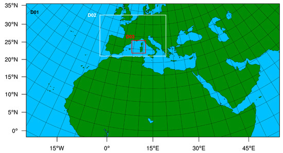
Figure 1.
Main and nested domains of simulations.
Table 2.
Primary configuration settings of the model.
3. Results
3.1. Description of the 20–25 June 2013 Synoptic Conditions
There are several variables that characterize synoptic weather conditions favorable to the dust mobilization. The most important variables are the geopotential height (usually at 500 hPa), the sea-level pressure and the surface winds. Well organized troughs (formations of low geopotential heights) lead to atmospheric instability conditions and downward momentum transport. Hence, a spatial pressure field is formed which is directly linked to the generation of significant pre and post frontal winds responsible for the dust triggering and transport [97]. The event of 20–25 June 2013 has been chosen, as it was associated with torrential rainfalls over Western Europe caused by a low-pressure system persistence over the Iberian Peninsula. On 19 June 2014 at 00 UTC (Figure 2a), a cut-off low over the Iberian Peninsula triggered baroclinic instability conditions. At that time, an extended frontal zone was located over Western France (Figure 2b). The prevailing SW winds ahead of the cold front at the tail of the frontal zone favored moisture advection from Western Mediterranean Sea and triggered torrential rainfall to Western France occurred on 21 June. This flow pattern also favored a large-scale desert dust transport from Algeria and Morocco and led to significant increase in dust load over Western Europe (Figure 3). Indeed, the simulated dust load presents local maxima of 3000 mg m−2 over the Western Mediterranean on 21 June at 12 UTC (Figure 4).
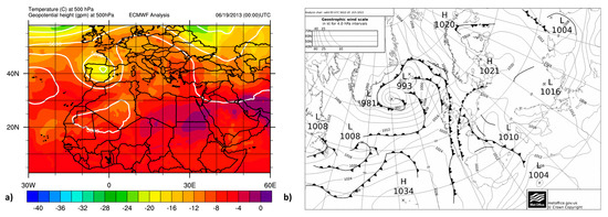
Figure 2.
(a) ECMWF gridded analysis of temperature (°C) and geopotential height (gpm) at 500 hPa for 19 June 2013 at 00 UTC. (b) Analysis of surface pressure (hPa) for 19 June 2013 at 00 UTC (source: UK Meteorological Office).
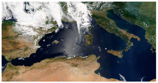
Figure 3.
Dust daily mobilization and transport to the Western Mediterranean for 20 June 2013 (source: WORLDVIEW–NASA).
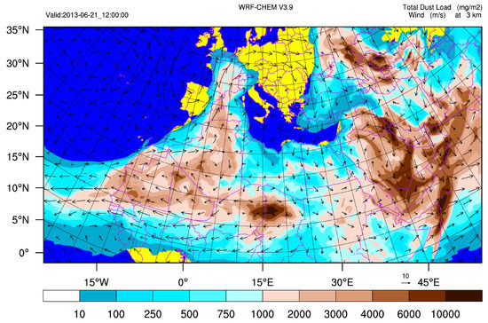
Figure 4.
Predicted dust load distribution (mg m−2) and wind speed (m s−1) at 3km for 21 June 2013 at 12 UTC.
3.2. Comparison of NCCN, Nc and RH
The average concentrations of CCN and cloud droplets of both CTRL and FN simulations as well as their differences (FN-CTRL) for 21 June 2013, 12 UTC, up to the height of 3 km and over D01 and D02 are shown in Figure 5. As expected, the CCN concentration (NCCN) of the FN run is in general much larger than the CTRL values, which are around 100 cm−3 (Figure 5a). On the other hand, FN simulation estimates that NCCN will reach 2000 cm−3 at the pathways of the severe dust advection over the Western Mediterranean (Figure 5b). The detected differences in NCCN are up to 1000 cm−3 over France (Figure 5c), showing a dominant hazy atmosphere at that time [91,98]. The total maxima of the NCCN differences are profoundly located over the dust sources (e.g., over Libya) areas reaching values of 4000 cm−3. In general, the NCCN concentrations are higher over land areas, especially over the areas that are considered as important aerosol sources [99,100].
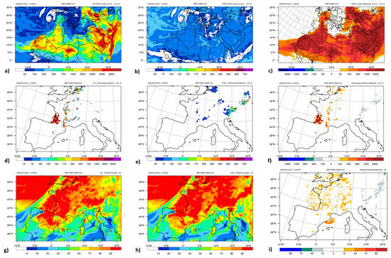
Figure 5.
Comparison of CCN concentration number, NCCN (cm−3), for (a) FN, (b) CTRL simulations and (c) FN-CTRL NCCN differences. Cloud droplet concentration number, NC (cm−3), for (d) FN, (e) CTRL simulations and (f) FN-CTRL NC differences. Relative humidity, RH (%), for (g) FN and (h) CTRL simulations and (i) FN-CTRL RH differences. All plots in this panel are valid for 21 June 2013 at 12 UTC.
The cloud droplet concentration (NC) estimated by FN simulation follows the NCCN pattern showing local maxima over 2000 cm−3 in the hazy atmosphere of South Western France (Figure 5d). The above results are comparable with those reported by [101,102], reporting that NC and NCCN maxima coincide as the last ones trigger the activation of more cloud droplets [25,98,102]. In the CTRL run (Figure 5e), however, NC presents a different to FN simulation pattern with the maxima of 300 cm−3 being located away from the areas influenced by the dust advection. This is because the overall NCCN and NC patterns in the FN run are altered by the mass preservation principle. Thus, the NC dominance in FN simulation over South Western France (Figure 5f) triggers the precipitation suppression 6 h later as the rain water becomes limited. Nc has also decreased over Central Europe by 400 cm−3 approximately, as this area is not characterized by significant dust advection. More specifically, NCCN of the FN run do not exceed 100 cm−3 and the prospect of a significant formation of NC is actually small. The relative humidity also plays an important role in the above mechanism. Figure 5g,h show the simulated relative humidity at FN and CTRL runs. In both runs, high values of relative humidity coincide with high or elevated NC concentrations. Figure 5i shows the FN-CTRL relative humidity differences. As expected over the area of South Western France, the relative humidity differences reach 30–50%. This increase coincides with the increase in the NC concentrations over the specific area. The abovementioned result confirms that high relative humidity creates favorable conditions for the cloud droplet activation [66,103]. Over Central Europe, the relative humidity is decreased up to 30%, contributing to the NC decrease over that specific area.
3.3. Impact on the Precipitation Pattern
Τhe increase in the CCN concentration due to the presence of dust particles affects the cloud condensation and the precipitation pattern. Figure 6a shows the D02 simulated 6h convective rainfall for the FN run, whereas Figure 6b indicates the convective rainfall differences of the FN against the CTRL run and the simulated CCN concentrations of the FN run in contours. The FN convective rainfall is enhanced by up to 6 mm over the marine areas of Western France and the Biscay Bay. This means that the prognostic treatment of the CCN embedded in the cumulus parameterization scheme enhances the convective rainfall over marine areas with lower CCN concentrations, which do not exceed the 50 cm−3 over the area of the Biscay Bay. In this case, the clouds rain out fast as large rain droplets are allowed to develop and the evaporation conditions are very limited [33,40,104]. On the contrary, in the FN run, a decrease in the convective precipitation by up to 8 mm is observed over the land areas of NE France, where a hazier atmosphere dominates as the CCN concentrations vary between 450 and 650 cm−3. Clouds in such environments are characterized by significant evaporation rates before the occurrence of precipitation [33]. Thus, the autoconversion of cloud to rain droplets and consequently to precipitation is very limited [40,105].
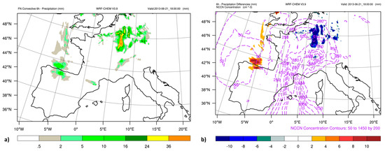
Figure 6.
(a) FN convective 6h precipitation (mm) and (b) 6h precipitation differences (mm) of FN against CTRL run for 21 June 2013 from 12:00–18:00 UTC (shaded) and FN NCCN concentrations (dashed lines) for 21 June 2103 at 18.00 UTC (contours).
To investigate the impact of the FN scheme to the non-convective rainfall, two areas in the D02 are selected, namely Areas 1,2 (Figure 7), as in these areas, significant suppression or enhancement of precipitation is noticed. Figure 8a shows the simulated 6h non-convective rainfall for the FN run whereas 8b shows the non-convective rainfall differences of the FN against the CTRL runs for the 21st June 2013 at 18.00 UTC. The suppression – enhancement precipitation mechanism is similar to the mechanism of the convective rainfall case. The non-convective rainfall is decreased by up to 8 mm over the area of Area 1 (Western France and NE Iberian Peninsula), where higher concentrations of CCN are simulated reaching values between 450 and 1050 cm−3. On the contrary, an enhancement in the precipitation up to 10 mm is observed over Area 2 (NE Germany and Central Poland), where CCN concentrations are significantly lower (50 cm−3 or less). The impact of the FN scheme on the precipitation some days after the dust transport event, on 24 June 2013 at 06.00 UTC, has been investigated through the FN simulated 6 h non-convective rainfall and the FN-CTRL rainfall differences (Figure 8c and Figure 8d respectively). Once more Area 2 is characterized by CCN concentrations ranging between 50 and 250 cm−3 and indicates an enhancement in the non-convective rainfall reaching 8 mm.
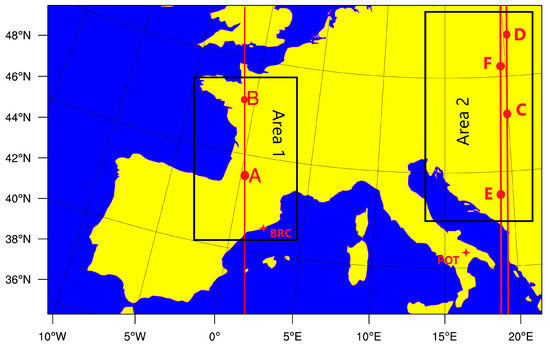
Figure 7.
Areas for the investigation of the FN impact on the non-convective precipitation. Longitudinal cross-section orientations for Area 1 (A,B) and Area 2 (C,D) and (E,F). Locations of LIDAR stations of Barcelona-Spain (BRC) and Potenza-Italy (POT).
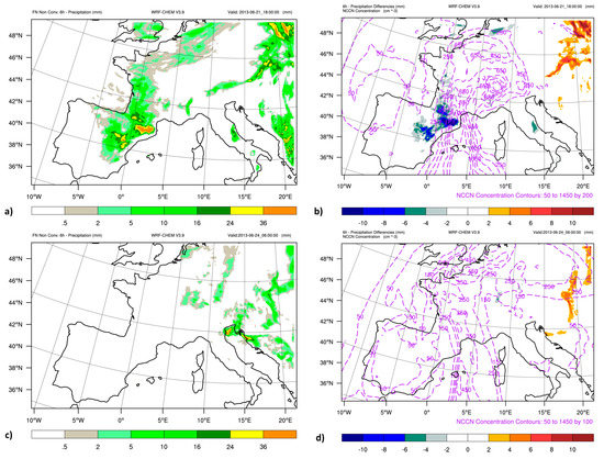
Figure 8.
(a) FN non-convective 6h precipitation (mm) and (b) 6 h non-convective precipitation differences (mm) of FN against CTRL run for 21 June, 2013 from 12.00–18.00 UTC (shaded) and FN NCCN concentrations for 21 June 2103 at 18.00 UTC (contours). (c) FN non-convective 6 h precipitation (mm) and (d) 6 h non-convective precipitation differences (mm) of FN against CTRL run for 24 June, 2013 from 00.00–06.00 UTC (shaded) and FN NCCN concentrations for 24 June 2103 at 06.00 UTC (contours).
The impact of the FN scheme to the non-convective precipitation pattern is furthermore investigated through vertical cross-sections of FN-CTRL differences of the cloud and rain water mixing ratios (mg kg−1). The cross-sections are in longitudinal orientation between points AB for Area 1 and points CD and EF for Area 2 (Figure 7). Figure 9a indicates that, for the AB area, for 21 June 2013 at 18.00 UTC, the FN enhancement to cloud water mixing ratio (shaded) reached values up to 400 mg kg−1. The increased cloud water mixing ratio is due to the higher CCN levels in the nearby areas, as it is shown in contours in Figure 9b (at least 450–500 cm−3). As is mentioned above, significant CCN concentrations in the atmosphere favor evaporation processes and limit the precipitation as the autoconversion of cloud to rain water becomes relatively poor [33,104,105]. Moreover, the high relative humidity (contour lines over 90%) also creates favorable conditions for the cloud water mixing ratio increase (Figure 9a). Due to the poor cloud to rain water autoconversion and the high cloud water mixing ratio, limited amounts of rain water are shown in Figure 9b as the rain water mixing ratio is decreased up to 400 mg kg−1, leading to the overall suppression of the precipitation for the area, as is also shown in Figure 8b. In the cross-section of Figure 9b, no decrease in the rain water in the lee side of the Pyrenees is observed, as the cross-section orientation does not include the area characterized by significant rainfall suppression (Figure 8b). The above procedure confirms the fact that cloud and rain water production are two inverse processes [106,107], highly dependent on the impact of the CCN to the atmospheric conditions.
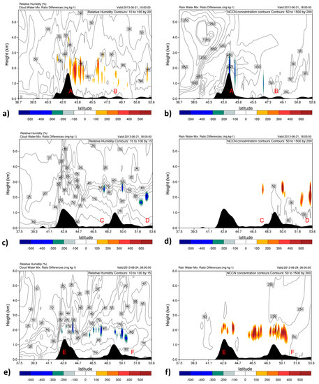
Figure 9.
Cross-section of cloud water mixing ratio differences (mg kg−1) (shaded) of the FN against CTRL run and relative humidity (%) (contours) for (a) 21 June 2013 at 18.00 UTC over Area AB, (c) 21 June 2013 at 18.00 UTC over Area CD and (e) for 24 June, 2013 at 06.00 UTC over Area EF. Cross-section of rain water mixing ratio differences (mg kg-1) of the FN against CTRL run (shaded) and FN NCCN contours (cm−3) for (b) 21 June 2013 at 18.00 UTC over Area AB, (d) for 21 June 2013 at 18.00 UTC over Area CD and (f) for 24 June 2013 at 06.00 UTC over Area EF.
Figure 9c shows the inverse procedure over Area CD with increased precipitation. In Figure 9c, the cloud water mixing ratio is decreased up to 500 mg kg−1 for 21 June, 2013 at 18.00 UTC. The cloud water mixing ratio is decreased as the specific area is not characterized by low amounts of CCN concentrations (approx. 50 cm−3, Figure 9d). This leads to high rates of cloud to rain water autoconversion [40,107] as fewer CCN antagonize the same amount of water. Furthermore, the lower relative humidity (50–70% approx.) also causes a weak effect of CCN. On the other hand, in Figure 9d the rain water mixing ratio is enhanced up to 500 mg kg−1 in the layer 2–3 km due to the accretion of cloud water [54].
Similar conditions occur in the EF area in Figure 9e,f for 24 June 2013 at 06.00 UTC, where the cloud water mixing ratio is suppressed, whereas the rain water mixing ratio and the overall precipitation are enhanced, under a low-relative-humidity environment.
In order to assess the impact of the FN scheme on the predictability of precipitation, an overall evaluation for both simulations is performed. The FN and CTRL bias scores, false alarm ratio (FAR) and frequencies of missed forecasts (FOM) of the simulated 24 h precipitation against the WORLDVIEW-NASA satellite retrievals (Atmospheric Infrared Sounder–AIRS–Level 2) are calculated for the Area 1 (AB–90 records) for 21 June, 2013 and Area 2 (CD–60 records, EF–52 records), for 21 and 24 June, 2013 (Table 2, Table 3 and Table 4, respectively). Nearest grid point value to the satellite ones are chosen.
Table 3.
FN and CTRL bias, FAR and FOM scores of the simulated 24 h precipitation against the AIRS (WORLDVIEW-NASA) satellite observations for Area AB, as is mentioned in Figure 7. The bold numbers indicate the certain thresholds in which the below scores have been estimated.
Table 4.
FN and CTRL bias, FAR and FOM scores of the simulated 24 h precipitation against the AIRS (WORLDVIEW-NASA) satellite observations for Area CD, as is mentioned in Figure 7. The bold numbers indicate the certain thresholds in which the below scores have been estimated.
The FN configuration improves generally the bias scores for the entire precipitation thresholds. In more details, over the area AB (Table 3) the systematic overprediction of CTRL for all precipitation thresholds is improved by the FN simulation as the bias scores are significantly reduced. FN also reduces the FAR in comparison to CTRL, which significantly overestimates the precipitation. FOM, however, does not appear any significant difference between the two schemes. As far as the areas CD (Table 4) and EF (Table 5) are concerned, the systematic underestimation in precipitation in the CTRL scheme is replaced by a slighter overestimation in the FN run. In general, the precipitation patterns, especially for heavy precipitation (e.g., at the 25 mm threshold), seem to be massively improved by the implementation of the FN scheme, which leads to an overall predictability improvement. However, for both areas, the FAR scores of the CTRL are better, especially for higher rainfall heights. On the contrary, the FN simulation significantly improves the FOM scores.
Table 5.
FN and CTRL bias, FAR and FOM scores of the simulated 24 h precipitation against the AIRS (WORLDVIEW-NASA) satellite observations for Area EF, as is mentioned in Figure 7. The bold numbers indicate the certain thresholds in which the below scores have been estimated.
3.4. Evaluation of the FN Scheme Through the Optical Properties.
A comparison is made between the estimated aerosol extinction coefficients of both FN and CTRL runs against the EARLINET’s network observations (Figure 10a,b, respectively). The stations of Barcelona (BRC) and Potenza (POT) have been selected (Figure 7) using a sample of 96 and 82 records, respectively. Figure 10a shows the comparison for BRC on the 25 June 2013 at 17.07 UTC. Although this date is away from the dust event, it was chosen not only due to the absence of any data set available on the days before (21–23) June, but also in order to demonstrate the impact of the FN implementation to the overall aerosol mass simulation a few days after the main event. An outlier in lidar measurements at 3500m of 0.9/km has been excluded from the statistical procedure. The comparison shows a clear overestimation of the CTRL aerosol extinction coefficient values, especially at the height of 1–5 km. This overestimation is significantly reduced by the FN scheme, as is shown in Table 6. The CTRL overestimation of the extinction coefficients could be attributed to the dust concentration overprediction computed by the GOCART/AFWA scheme [85,89,108]. The CTRL bias of 0.07 reduces to 0.013 for the FN run. The root mean square error (RMSE) is also improved as the CTRL RMSE value of 0.17 is reduced to 0.14 for the FN simulation.
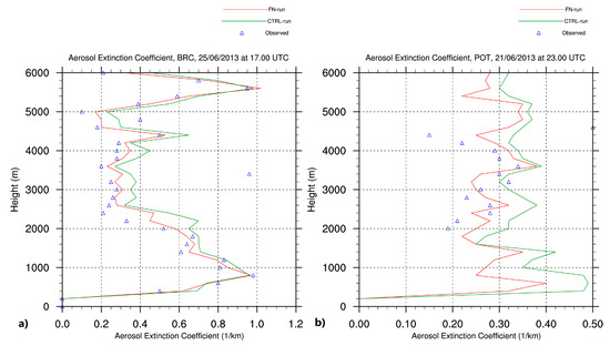
Figure 10.
Comparison between the estimated aerosol extinction coefficients of both FN and CTRL runs against the LIDAR EARLINET’s network observations for (a) BRC (Barcelona) on 25 June 2013, at 17.07 UTC and (b) POT (Potenza) on 21 June 2013, at 22.47 UTC.
Table 6.
Bias and RMSE between simulated aerosol extinction coefficient (1/km) (FN and CTRL) and observed aerosol extinction coefficient (LIDAR–EARLINET network) for the BRC (Barcelona) station.
The comparison for the Potenza station on 21 June 2013 at 22.47 UTC (Figure 10b) indicates similar results. Once more the CTRL overestimation is reduced by the FN simulation. However, the differences here are greater. The outlier value of 0.14/km near the level of 4500 m has also been excluded from the comparison. Table 6 and Table 7 show the bias and the RMSE differences for BRC and POT, respectively. For BRC, the CTRL overestimation is improved by the FN simulation, as the CTRL bias of 0.070 is clearly reduced to the FN bias value of 0.13. However, there is a systematic overestimation from both simulations over both sites. This may be attributed to the fact that AFWA generally overestimates the dust aerosol concentration as it takes into account higher amounts of clay, at the dust sources parameterizations [85,108]. Furthermore, the observation and the simulation data are derived at the wavelength of 530 nm. This presents a degree of uncertainty because the correlation between the aerosol extinction coefficient and the CCN concentrations could be more satisfactory in lower wavelengths [109]. The CTRL RMSE value of 0.17 is also reduced to 0.14 in the FN scheme. Similarly, for POT, the CTRL overestimation is significantly improved by the FN simulation, as the CTRL bias value of 0.041 is reduced to 0.028. Similarly, the CTRL RMSE value of 0.066 is also reduced to 0.048. However, in the level of 4–4.5 km, an observation value presents a sudden drop reaching 0.15 km−1. This value cannot be considered as reliable and is not taken into account.
Table 7.
Bias and RMSE between simulated aerosol extinction coefficient (1/km) (FN and CTRL) and observed aerosol extinction coefficient (LIDAR–EARLINET network) for the POT (Potenza) station.
3.5. Estimation of CCN vVertical Profiles and Comparison with Observational Data
The performance of the implemented FN scheme is also evaluated through a comparison between vertical profiles of CCN concentrations (cm−3) measured by aircraft (SAFIRE/MNPCA-CNRM/GAME) and those simulated by the FN (red line) and CTRL (green line) runs over eastern Sardinia (Domain 03) on 22 June 2013 at 10 UTC. Figure 11 shows the locations of the aircraft measurements, while the mean geographic location of the aircraft for each sampling period is considered, in a sample of 180 records. The simulated CCN concentration for each corresponding location is calculated as the weighted average from the nearest grid point of the model. FN simulation estimates considerably higher concentrations than the CTRL (Figure 12). The FN configuration reproduces in a similar way to the observed CCN profile, with an overestimation of approximately 400–500 cm−3 mainly at heights above the atmospheric boundary layer (1000–3000 m). The excess of the estimated CCN concentration by FN simulation is directly linked to the systematic overestimation of the dust concentration by the GOCART-AFWA scheme [89,108]. Table 8 shows the bias and the RMSE differences between the FN and the CTRL runs. The underestimation of the CTRL simulation by about 280 cm−3 turns to overestimation of FN simulation by 38 cm−3. The implementation of the FN scheme also massively improves the error of the model with 125 cm−3 instead of 358 cm−3. Additionally, FN also improves the correlation coefficient against the aircraft observations reaching 0.93, as is shown in Figure 13 (green color–solid line).
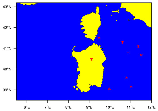
Figure 11.
Locations of CCN concentration number aircraft measurements.
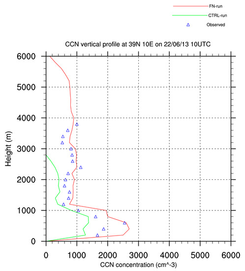
Figure 12.
Comparison between vertical profiles of values of observed CCN concentrations (cm−3) with the activated CCN concentrations simulated by the FN (red line) and the CTRL (green line) runs.
Table 8.
Bias and RMSE between simulated activated CCN concentration (cm−3) (FN and CTRL) and observed CCN concentration (aircraft-SAFIRE/MNPCA-CNRM/GAME) for the location of Sardinia.
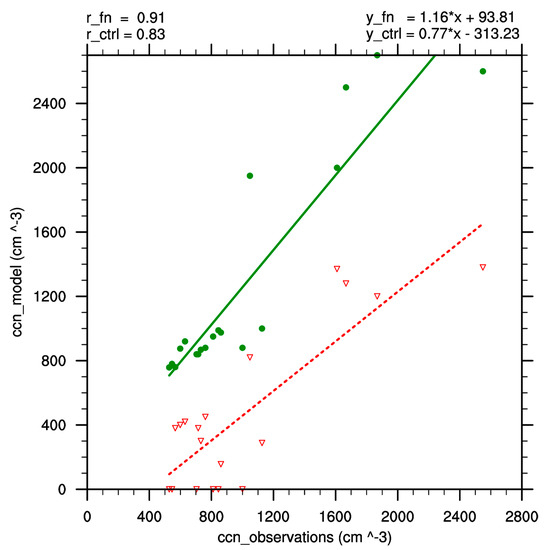
Figure 13.
Comparison between the correlation coefficients of both (a) FN (green) and (b) CTRL (red) simulations against the aircraft observations data (SAFIRE/MNPCA-CNRM/GAME).
4. Discussion and Conclusions
The potential indirect effects of desert dust aerosols on cloud formation and precipitation have been investigated in this study through the implementation of the revised Fountoukis and Nenes [55] cloud nucleation scheme (FN scheme) in the fully coupled meteorology–chemistry model WRF/Chem. The impact of the above nucleation scheme on both the WDM6 [13,66] double-moment microphysics scheme and the Grell and Freitas [51] cumulus scheme has been taken into account. Dust CCN dynamical impacts were assessed in an extreme Saharan dust outbreak over the Western Mediterranean and Europe accompanied by torrential rainfall on 20–25 June, 2013. Two experiments having as a basis the GOCART-AFWA module with the FN scheme or with the default configuration have been conducted.
As far as convective clouds are concerned, the treatment of CCN based on prognostic dust particles suppresses precipitation over hazy areas, characterized by significant evaporation and limited cloud to rain droplet conversion. More specifically, clouds in such environments are characterized by significant evaporation rates before the precipitation has occurred [33]. Furthermore, in spite of a CCN increase, the same amount of water is distributed among the particles. Thus, the concentration of cloud droplets is increased but their diameters are reduced. In this case, the transformation time of cloud to rain drops increases, especially during the early stages of the cloud formation. Hence, the autoconversion mechanism of cloud to rain droplets and also the precipitation becomes very limited [40,105]. Furthermore, cloud reflectivity is enhanced as cloud surface increases. On the other hand, convective rainfall in a clean atmosphere is enhanced as the exact inverse procedure is occurred. In such cases, the cloud rain out acts very quickly as evaporation is limited.
The non-convective precipitation mechanisms follow a similar enhancement–suppression pattern as above. Hazy environments limit precipitation as high CCN levels lead to significant amounts of cloud water and poor conversion rates of cloud to rain water mixing ratios [33,104,105]. Apart from the enhanced evaporation, high amounts of relative humidity contribute to the above mechanism. On the contrary, pristine conditions lead to the exact opposite results, as limited evaporation conditions, lower relative humidity amounts and decreased cloud water mixing ratios lead to important cloud to rain water conversion and enhancement of precipitation [106,107]. It is remarkable that the prognostic treatment of dust particles enhances significantly the precipitation over areas far away from the dust event. Enhancement of the precipitation over those areas has also been noticed some days after the event.
Comparison of FN and CTRL results of precipitation, extinction coefficients and CCN levels against observations indicated that the FN scheme generally improves the forecasting skill of the model. Bias and RMSE scores are limited in overall as the FN simulation is better correlated with the observed data. CTRL run overestimates precipitation over hazy areas and underestimates it over pristine areas showing important biases especially for thresholds of large precipitation heights. Those biases are improved by the implemented FN scheme, which suppresses the precipitation over the polluted areas and enhances it in clear atmospheric conditions. Concerning hazy areas, the FN simulation improves the FAR scores but does not significantly affect the FOM scores. In pristine areas, however, CTRL has a better performance concerning the FAR. FOM on the other hand improves significantly by the FN simulation. The above result indicates that prognostic CCN treatment is important for both hazy and pristine areas, as it alters the overall precipitation pattern. Furthermore, as far as the extinction coefficient is concerned, the CTRL overestimation is limited by the FN simulation. Moreover, the CCN underprediction on behalf of the CTRL simulation turns to a slight overprediction by the FN run.
The systematic overprediction of both the extinction coefficient and the CCN concentration may be attributed to the overestimation of the GOCART/AFWA scheme in dust aerosol levels. However, this overprediction, as well as the overestimation in precipitation, may also be attributed to the fact that the FN simulation takes into account only prognostic dust particles, since prognostic sea salt particles or other aerosols are neglected in this study. The impact of sea salt aerosols on the model performance is a plan of further investigation.
Author Contributions
K.T. contributed to the methodology and formal analysis, investigation, visualization and writing original draft; P.K. contributed to the conceptualization, methodology, supervision, investigation, writing, review and editing; A.P.; N.M. contributed to the investigation, writing, review and editing. All authors have read and agreed to the published version of the manuscript.
Funding
This research received no external funding.
Acknowledgments
We acknowledge support of this work by the project “PANhellenic infrastructure for Atmospheric Composition and climatE change” (MIS 5021516) which is implemented under the Action “Reinforcement of the Research and Innovation Infrastructure”, funded by the Operational Programme “Competitiveness, Entrepreneurship and Innovation” (NSRF 2014–2020) and co-financed by Greece and the European Union (European Regional Development Fund). We also gratefully thank the aircraft and instrument operation by SAFIRE, data processing by the MNPCA team of CNRM-GAME, project initiation and coordination by M. Mallet and F. Dulac, and funding by ANR ADRIMED (contract ANR-11-BS56-0006)/CNES TOSCA/MISTRALS. We acknowledge the use of imagery from the NASA Worldview application (https://worldview.earthdata.nasa.gov/) operated by the NASA/Goddard Space Flight Center Earth Science Data and Information System (EOSDIS) project. British Meteorological Office is also acknowledged for the provision of the surface analysis charts. The authors acknowledge EARLINET for providing aerosol lidar profiles (www.earlinet.org). We also acknowledge the Atmospheric Infrared Sounder (AIRS–Level 2, https://airsl2.gesdisc.eosdis.nasa.gov) for providing precipitation data.
Conflicts of Interest
The authors declare no conflict of interest.
References
- Andreae, M.O.; Charlson, R.J.; Bruynseels, F.; Storms, H.; VAN Grieken, R.; Maenhaut, W. Internal Mixture of Sea Salt, Silicates, and Excess Sulfate in Marine Aerosols. Science 1986, 232, 1620–1623. [Google Scholar] [CrossRef] [PubMed]
- Zender, C.S.; Miller, R.L.; Tegen, I. Quantifying Mineral Dust Mass Budgets: Terminology, Constraints, and Current Estimates. Eos 2004, 85, 509–512. [Google Scholar] [CrossRef]
- Ben-Ami, Y.; Koren, I.; Altaratz, O. Patterns of North African Dust Transport over the Atlantic: Winter vs. Summer, Based on CALIPSO First Year Data. Atmos. Chem. Phys. 2009, 9, 7867–7875. [Google Scholar] [CrossRef]
- Kaufman, Y.J.; Tanré, D.; Boucher, O. A Satellite View of Aerosols in the Climate System. Nature 2002, 419, 215–223. [Google Scholar] [CrossRef] [PubMed]
- Nenes, A.; Charlson, R.J.; Facchini, M.C.; Kulmala, M.; Laaksonen, A.; Seinfeld, J.H. Can Chemical Effects on Cloud Droplet Number Rival the First Indirect Effect? Geophys. Res. Lett. 2002, 29, 29-1–29-4. [Google Scholar] [CrossRef]
- Perlwitz, J.; Tegen, I.; Miller, R.L. Interactive Soil Dust Aerosol Model in the GISS GCM 1. Sensitivity of the Soil Dust Cycle to Radiative Properties of Soil Dust Aerosols. J. Geophys. Res. Atmos. 2001, 106, 18167–18192. [Google Scholar] [CrossRef]
- Myhre, G.; Grini, A.; Haywood, J.M.; Stordal, F.; Chatenet, B.; Tanré, D.; Sundet, J.K.; Isaksen, I.S.A. Modeling the Radiative Impact of Mineral Dust during the Saharan Dust Experiment (SHADE) Campaign. J. Geophys. Res. D Atmos. 2003, 108, 1–13. [Google Scholar] [CrossRef]
- Ramanathan, V.; Ramana, M.V.; Roberts, G.; Kim, D.; Corrigan, C.; Chung, C.; Winker, D. Warming Trends in Asia Amplified by Brown Cloud Solar Absorption. Nature 2007, 448, 575–578. [Google Scholar] [CrossRef]
- Pérez, C.; Nickovic, S.; Baldasano, J.M.; Sicard, M.; Rocadenbosch, F.; Cachorro, V.E. A Long Saharan Dust Event over the Western Mediterranean: Lidar, Sun Photometer Observations, and Regional Dust Modeling. J. Geophys. Res. Atmos. 2006, 111, D15214. [Google Scholar] [CrossRef]
- Heinold, B.; Tegen, I.; Schepanski, K.; Hellmuth, O. Dust Radiative Feedback on Saharan Boundary Layer Dynamics and Dust Mobilization. Geophys. Res. Lett. 2008, 35, L20817. [Google Scholar] [CrossRef]
- Lau, K.M.; Kim, M.K.; Kim, K.M. Asian Summer Monsoon Anomalies Induced by Aerosol Direct Forcing: The Role of the Tibetan Plateau. Clim. Dyn. 2006, 26, 855–864. [Google Scholar] [CrossRef]
- Lau, K.M.; Kim, K.M.; Sud, Y.C.; Walker, G.K. A GCM Study of the Response of the Atmospheric Water Cycle of West Africa and the Atlantic to Saharan Dust Radiative Forcing. Ann. Geophys. 2009, 27, 4023–4037. [Google Scholar] [CrossRef]
- Lim, K.S.S.; Hong, S.Y. Development of an Effective Double-Moment Cloud Microphysics Scheme with Prognostic Cloud Condensation Nuclei (CCN) for Weather and Climate Models. Mon. Weather Rev. 2010, 138, 1587–1612. [Google Scholar] [CrossRef]
- Herut, B.; Collier, R.; Krom, M.D. The Role of Dust in Supplying Nitrogen and Phosphorus to the Southeast Mediterranean. Limnol. Oceanogr. 2002, 47, 870–878. [Google Scholar] [CrossRef]
- Spyrou, C.; Mitsakou, C.; Kallos, G.; Louka, P.; Vlastou, G. An Improved Limited Area Model for Describing the Dust Cycle in the Atmosphere. J. Geophys. Res. Atmos. 2010, 115, D17211. [Google Scholar] [CrossRef]
- Meskhidze, N.; Chameides, W.L.; Nenes, A. Dust and Pollution: A Recipe for Enhanced Ocean Fertilization? J. Geophys. Res. D Atmos. 2005, 110, D03301. [Google Scholar] [CrossRef]
- Mahowald, N.; Jickells, T.D.; Baker, A.R.; Artaxo, P.; Benitez-Nelson, C.R.; Bergametti, G.; Bond, T.C.; Chen, Y.; Cohen, D.D.; Herut, B.; et al. Global Distribution of Atmospheric Phosphorus Sources, Concentrations and Deposition Rates, and Anthropogenic Impacts. Glob. Biogeochem. Cycles 2008, 22, GB4026. [Google Scholar] [CrossRef]
- Lelieveld, J.; Evans, J.S.; Fnais, M.; Giannadaki, D.; Pozzer, A. The Contribution of Outdoor Air Pollution Sources to Premature Mortality on a Global Scale. Nature 2015, 525, 367–371. [Google Scholar] [CrossRef]
- Prospero, J.M. Saharan Dust Transport Over the North Atlantic Ocean and Mediterranean: An Overview BT. In The Impact of Desert Dust Across the Mediterranean; Guerzoni, S., Chester, R., Eds.; Springer: Dordrecht, The Netherlands, 1996; pp. 133–151. [Google Scholar] [CrossRef]
- Twomey, S. The Nuclei of Natural Cloud Formation Part II: The Supersaturation in Natural Clouds and the Variation of Cloud Droplet Concentration. Geofis. Pura E Appl. 1959, 43, 243–249. [Google Scholar] [CrossRef]
- Albrecht, B.A. Aerosols, Cloud Microphysics, and Fractional Cloudiness. Science 1989, 245, 1227–1230. [Google Scholar] [CrossRef] [PubMed]
- DeMott, P.J.; Prenni, A.J.; Liu, X.; Kreidenweis, S.M.; Petters, M.D.; Twohy, C.H.; Richardson, M.S.; Eidhammer, T.; Rogers, D.C. Predicting Global Atmospheric Ice Nuclei Distributions and Their Impacts on Climate. Proc. Natl. Acad. Sci. USA 2010, 107, 11217–11222. [Google Scholar] [CrossRef] [PubMed]
- Sassen, K.; DeMott, P.J.; Prospero, J.M.; Poellot, M.R. Saharan Dust Storms and Indirect Aerosol Effects on Clouds: CRYSTAL-FACE Results. Geophys. Res. Lett. 2003, 30, 1–4. [Google Scholar] [CrossRef]
- Andreae, M.O.; Rosenfeld, D. Aerosol-Cloud-Precipitation Interactions. Part 1. The Nature and Sources of Cloud-Active Aerosols. Earth-Sci. Rev. 2008, 89, 13–41. [Google Scholar] [CrossRef]
- Twomey, S. The Influence of Pollution on the Shortwave Albedo of Clouds. J. Atmos. Sci. 1977, 34, 1149–1152. [Google Scholar] [CrossRef]
- Kaufman, Y.J.; Koren, I.; Remer, L.A.; Rosenfeld, D.; Rudich, Y. The Effect of Smoke, Dust, and Pollution Aerosol on Shallow Cloud Development over the Atlantic Ocean. Proc. Natl. Acad. Sci. USA 2005, 102, 11207–11212. [Google Scholar] [CrossRef]
- Teller, A.; Levin, Z. The Effects of Aerosols on Precipitation and Dimensions of Subtropical Clouds: A Sensitivity Study Using a Numerical Cloud Model. Atmos. Chem. Phys. 2006, 6, 67–80. [Google Scholar] [CrossRef]
- Pincus, R.; Baker, M.B. Effect of Precipitation on the Albedo Susceptibility of Clouds in the Marine Boundary Layer. Nature 1994, 372, 250–252. [Google Scholar] [CrossRef]
- Hansen, J.; Sato, M.; Ruedy, R. Radiative Forcing and Climate Response. J. Geophys. Res. 1997, 102, 6831–6864. [Google Scholar] [CrossRef]
- Fernández-González, S.; Wang, P.K.; Gascón, E.; Valero, F.; Sánchez, J.L. Latent Cooling and Microphysics Effects in Deep Convection. Atmos. Res. 2016, 180, 189–199. [Google Scholar] [CrossRef]
- Khain, A.; Pokrovsky, A.; Pinsky, M.; Seifert, A.; Phillips, V. Simulation of Effects of Atmospheric Aerosols on Deep Turbulent Convective Clouds Using a Spectral Microphysics Mixed-Phase Cumulus Cloud Model. Part I: Model Description and Possible Applications. J. Atmos. Sci. 2004, 61, 2963–2982. [Google Scholar] [CrossRef]
- Cotton, W.R.; Zhang, H.; McFarquhar, G.M.; Saleeby, S.M. Should We Consider Polluting Hurricanes to Reduce Their Intensity? J. Weather Modif. 2007, 39, 70–73. [Google Scholar]
- Rosenfeld, D.; Lohmann, U.; Raga, G.B.; O’Dowd, C.D.; Kulmala, M.; Fuzzi, S.; Reissell, A.; Andreae, M.O. Flood or Drought: How Do Aerosols Affect Precipitation? Science 2008, 321, 1309–1313. [Google Scholar] [CrossRef] [PubMed]
- Khain, A.; Rosenfeld, D.; Pokrovsky, A. Aerosol Impact on the Dynamics and Microphysics of Deep Convective Clouds. Q. J. R. Meteorol. Soc. 2005, 131, 2639–2663. [Google Scholar] [CrossRef]
- Lebo, Z.J.; Morrison, H.; Seinfeld, J.H. Are Simulated Aerosol-Induced Effects on Deep Convective Clouds Strongly Dependent on Saturation Adjustment? Atmos. Chem. Phys. 2012, 12, 9941–9964. [Google Scholar] [CrossRef]
- Andreae, M.O.; Rosenfeld, D.; Artaxo, P.; Costa, A.A.; Frank, G.P.; Longo, K.M.; Silva-Dias, M.A.F. Smoking Rain Clouds over the Amazon. Science 2004, 303, 1337–1342. [Google Scholar] [CrossRef]
- Koren, I.; Remer, L.A.; Altaratz, O.; Martins, J.V.; Davidi, A. Aerosol-Induced Changes of Convective Cloud Anvils Produce Strong Climate Warming. Atmos. Chem. Phys. 2010, 10, 5001–5010. [Google Scholar] [CrossRef]
- Niu, F.; Li, Z. Systematic Variations of Cloud Top Temperature and Precipitation Rate with Aerosols over the Global Tropics. Atmos. Chem. Phys. 2012, 12, 8491–8498. [Google Scholar] [CrossRef]
- Charlson, R.J.; Seinfeld, J.H.; Nenes, A.; Kulmala, M.; Laaksonen, A.; Facchini, M.C. Atmospheric Science. Reshaping the Theory of Cloud Formation. Science 2001, 292, 2025–2026. [Google Scholar] [CrossRef]
- Solomos, S.; Kallos, G.; Kushta, J.; Astitha, M.; Tremback, C.; Nenes, A.; Levin, Z. An Integrated Modeling Study on the Effects of Mineral Dust and Sea Salt Particles on Clouds and Precipitation. Atmos. Chem. Phys. 2011, 11, 873–892. [Google Scholar] [CrossRef]
- Yin, Y.; Chen, L. The Effects of Heating by Transported Dust Layers on Cloud and Precipitation: A Numerical Study. Atmos. Chem. Phys. 2007, 7, 3497–3505. [Google Scholar] [CrossRef]
- Wilcox, E.M. Direct and Semi-Direct Radiative Forcing of Smoke Aerosols over Clouds. Atmos. Chem. Phys. 2012, 12, 139–149. [Google Scholar] [CrossRef]
- Lynn, B.; Khain, A.; Rosenfeld, D.; Woodley, W.L. Effects of Aerosols on Precipitation from Orographic Clouds. J. Geophys. Res. Atmos. 2007, 112, D10225. [Google Scholar] [CrossRef]
- Zhang, H.; McFarquhar, G.M.; Saleeby, S.M.; Cotton, W.R. Impacts of Saharan Dust as CCN on the Evolution of an Idealized Tropical Cyclone. Geophys. Res. Lett. 2007, 34, L14812. [Google Scholar] [CrossRef]
- Menon, S.; Del Genio, A.D.; Koch, D.; Tselioudis, G. GCM Simulations of the Aerosol Indirect Effect: Sensitivity to Cloud Parameterization and Aerosol Burden. J. Atmos. Sci. 2002, 59, 692–713. [Google Scholar] [CrossRef]
- Ghan, S.J.; Easter, R.C.; Chapman, E.G.; Abdul-Razzak, H.; Zhang, Y.; Leung, L.R.; Laulainen, N.S.; Saylor, R.D.; Zaveri, R.A. A Physically Based Estimate of Radiative Forcing by Anthropogenic Sulfate Aerosol. J. Geophys. Res. Atmos. 2001, 106, 5279–5293. [Google Scholar] [CrossRef]
- Khain, A.P.; BenMoshe, N.; Pokrovsky, A. Factors Determining the Impact of Aerosols on Surface Precipitation from Clouds: An Attempt at Classification. J. Atmos. Sci. 2008, 65, 1721–1748. [Google Scholar] [CrossRef]
- Khain, A. Simulation of a Supercell Storm in Clean and Dirty Atmosphere Using Weather Research and Forecast Model with Spectral Bin Microphysics. J. Geophys. Res. Atmos. 2009, 114, 11419. [Google Scholar] [CrossRef]
- Han, J.-Y.; Baik, J.-J.; Lee, H. Urban Impacts on Precipitation. Asia-Pac. J. Atmos. Sci. 2014, 50, 17–30. [Google Scholar] [CrossRef]
- Lerach, D.G.; Gaudet, B.J.; Cotton, W.R. Idealized Simulations of Aerosol Influences on Tornadogenesis. Geophys. Res. Lett. 2008, 35, 1–6. [Google Scholar] [CrossRef]
- Wang, C.A. Modeling Study of the Response of Tropical Deep Convection to the Increase of Cloud Condensation Nuclei Concentration: 1. Dynamics and Microphysics. J. Geophys. Res. Atmos. 2005, 110, D21211. [Google Scholar] [CrossRef]
- Grell, G.A.; Freitas, S.R. A Scale and Aerosol Aware Stochastic Convective Parameterization for Weather and Air Quality Modeling. Atmos. Chem. Phys. 2014, 14, 5233–5250. [Google Scholar] [CrossRef]
- Berg, L.K.; Shrivastava, M.; Easter, R.C.; Fast, J.D.; Chapman, E.G.; Liu, Y.; Ferrare, R.A. A New WRF-Chem Treatment for Studying Regional-Scale Impacts of Cloud Processes on Aerosol and Trace Gases in Parameterized Cumuli. Geosci. Model Dev. 2015, 8, 409–429. [Google Scholar] [CrossRef]
- Kang, J.Y.; Bae, S.Y.; Park, R.S.; Han, J.Y. Aerosol Indirect Effects on the Predicted Precipitation in a Global Weather Forecasting Model. Atmosphere 2019, 10, 392. [Google Scholar] [CrossRef]
- Fountoukis, C.; Nenes, A. Continued Development of a Cloud Droplet Formation Parameterization for Global Climate Models. J. Geophys. Res. D Atmos. 2005, 110, D11212. [Google Scholar] [CrossRef]
- Skamarock, W.C.; Klemp, B.J.; Dudhia, J.; Gill, D.O.; Barker, D.M.; Duda, M.G.; Huang, X.-Y.; Wang, W.; Powers, J.G. A Description of the Advanced Research WRF Version 3, NCAR Tech. Note, NCAR/TN-468+STR; National Center for Atmospheric Research: Boulder, CO, USA, 2008. [Google Scholar] [CrossRef]
- Grell, G.A.; Peckham, S.E.; Schmitz, R.; McKeen, S.A.; Frost, G.; Skamarock, W.C.; Eder, B. Fully Coupled “Online” Chemistry within the WRF Model. Atmos. Environ. 2005, 39, 6957–6975. [Google Scholar] [CrossRef]
- Kessler, E. On the Distribution and Continuity of Water Substance in Atmospheric Circulations; Kessler, E., Ed.; American Meteorological Society: Boston, MA, USA, 1969; pp. 1–84. [Google Scholar] [CrossRef]
- Lin, Y.-L.; Farley, R.; Orville, H. Bulk Parameterization of the Snow Field in a Cloud Model. J. Appl. Meteorol. 1983, 22, 1065–1092. [Google Scholar] [CrossRef]
- Ferrier, B.S.; Jin, Y.; Lin, Y.; Black, T.; Rogers, E.; Dimego, G. Implementation of a New Grid-Scale Cloud and Precipitation Scheme in the NCEP Eta Model. In Proceedings of the 15th Conference on Numerical Weather Prediction, State College, PA, USA, 11 August 2002; pp. 280–283. [Google Scholar]
- Hong, S.-Y.; Kim, J.-H.; Lim, J.; Dudhia, J. The WRF Single Moment Microphysics Scheme (WSM). J. Korean Meteorol. Soc. 2006, 42, 129–151. [Google Scholar]
- Thompson, G.; Field, P.R.; Rasmussen, R.M.; Hall, W.D. Explicit Forecasts of Winter Precipitation Using an Improved Bulk Microphysics Scheme. Part II: Implementation of a New Snow Parameterization. Mon. Weather Rev. 2008, 136, 5095–5115. [Google Scholar] [CrossRef]
- Morrison, H.; Thompson, G.; Tatarskii, V. Impact of Cloud Microphysics on the Development of Trailing Stratiform Precipitation in a Simulated Squall Line: Comparison of One- and Two-Moment Schemes. Mon. Weather Rev. 2009, 137, 991–1007. [Google Scholar] [CrossRef]
- Milbrandt, J.A.; Yau, M.K. A Multimoment Bulk Microphysics Parameterization. Part I: Analysis of the Role of the Spectral Shape Parameter. J. Atmos. Sci. 2005, 62, 3051–3064. [Google Scholar] [CrossRef]
- Milbrandt, J.A.; Yau, M.K. A Multimoment Bulk Microphysics Parameterization. Part II: A Proposed Three-Moment Closure and Scheme Description. J. Atmos. Sci. 2005, 62, 3065–3081. [Google Scholar] [CrossRef]
- Shi, Z.; Tan, Y.; Liu, Y.; Liu, J.; Lin, X.; Wang, M.; Luan, J. Effects of Relative Humidity on Electrification and Lightning Discharges in Thunderstorms. Terr. Atmos. Ocean. Sci. 2018, 29, 695–708. [Google Scholar] [CrossRef]
- Hong, S.-Y.; Lim, K.-S.S.; Lee, Y.-H.; Ha, J.-C.; Kim, H.-W.; Ham, S.-J.; Dudhia, J. Evaluation of the WRF Double-Moment 6-Class Microphysics Scheme for Precipitating Convection. Adv. Meteorol. 2010, 2010, 707253. [Google Scholar] [CrossRef]
- Reddy, M.V.; Prasad, S.B.S.; Krishna, U.V.M.; Reddy, K.K. Effect of Cumulus and Microphysical Parameterizations on the JAL Cyclone Prediction. Indian J. Radio Space Phys. 2014, 43, 103–123. [Google Scholar]
- Mayor, Y.G.; Mesquita, M.D.S. Numerical Simulations of the 1 May 2012 Deep Convection Event over Cuba: Sensitivity to Cumulus and Microphysical Schemes in a High-Resolution Model. Adv. Meteorol. 2015, 2015. [Google Scholar] [CrossRef]
- Hong, S.Y.; Dudhia, J.; Chen, S.H. A Revised Approach to Ice Microphysical Processes for the Bulk Parameterization of Clouds and Precipitation. Mon. Weather Rev. 2004, 132, 103–120. [Google Scholar] [CrossRef]
- Morrison, H.; Milbrandt, J.A. Parameterization of Cloud Microphysics Based on the Prediction of Bulk Ice Particle Properties. Part I: Scheme Description and Idealized Tests. J. Atmos. Sci. 2015, 72, 287–311. [Google Scholar] [CrossRef]
- Cohard, J.-M.; Pinty, J.-P. A Comprehensive Two-Moment Warm Microphysical Bulk Scheme. I: Description and Tests. Q. J. R. Meteorol. Soc. 2000, 126, 1815–1842. [Google Scholar] [CrossRef]
- Khairoutdinov, M.; Kogan, Y. A New Cloud Physics Parameterization in a Large-Eddy Simulation Model of Marine Stratocumulus. Mon. Weather Rev. 2000, 128, 229–243. [Google Scholar] [CrossRef]
- Nenes, A.; Seinfeld, J.H. Parameterization of Cloud Droplet Formation in Global Climate Models. J. Geophys. Res. Atmos. 2003, 108, 1–14. [Google Scholar] [CrossRef]
- Seinfeld, J.H.; Pandis, S.N.; Noone, K. Atmospheric Chemistry and Physics: From Air Pollution to Climate Change. Phys. Today 1998, 51, 88. [Google Scholar] [CrossRef]
- Krikken, F.; Steeneveld, G. Modelling the re-intensification of tropical storm Erin (2007) over Oklahoma: Understanding the key role of downdraft formulation. Tellus A Dyn. Meteorol. Oceanogr. 2012, 64, 61. [Google Scholar] [CrossRef]
- Freitas, S.R.; Grell, G.A.; Molod, A.; Thompson, M.A.; Putman, W.M.; Santos e Silva, C.M.; Souza, E.P. Assessing the Grell-Freitas Convection Parameterization in the NASA GEOS Modeling System. J. Adv. Model. Earth Syst. 2018, 10, 1266–1289. [Google Scholar] [CrossRef] [PubMed]
- Chin, M.; Rood, R.B.; Lin, S.J.; Müller, J.F.; Thompson, A.M. Atmospheric Sulfur Cycle Simulated in the Global Model GOCART: Model Description and Global Properties. J. Geophys. Res. Atmos. 2000, 105, 24671–24687. [Google Scholar] [CrossRef]
- Ginoux, P.; Chin, M.; Tegen, I.; Goddard, T.; Prospero, J.M.; Holben, B.; Dubovik, O.; Lin, S.-J. Sources and distributions of dust aerosols simulated with the GOCART model. J. Geophys. Res. 2001, 106, 20255–20273. [Google Scholar] [CrossRef]
- Jones, S.L.; Creighton, G.A.; Kuchera, E.L.; Rentschler, S.A. Adapting WRF-CHEM GOCART for Fine-Scale Dust Forecasting. In AGU Fall Meeting Abstracts; 2011; Volume 2011, p. U14A-06. Available online: https://ui.adsabs.harvard.edu/abs/2011AGUFM.U14A..06J/abstract (accessed on 7 September 2020).
- Jones, S.L.; Adams-Selin, R.; Hunt, E.D.; Creighton, G.A.; Cetola, J.D. Update on Modifications to WRF-CHEM GOCART for Fine-Scale Dust Forecasting at AFWA. In AGU Fall Meeting Abstracts; 2012; Volume 2012, p. A33D-0188. Available online: https://ui.adsabs.harvard.edu/abs/2012AGUFM.A33D0188J/abstract (accessed on 7 September 2020).
- Marticorena, B.; Bergametti, G. Modeling the Atmospheric Dust Cycle: 1. Design of a Soil-Derived Dust Emission Scheme. J. Geophys. Res. Atmos. 1995, 100, 16415–16430. [Google Scholar] [CrossRef]
- LeGrand, S.L.; Polashenski, C.; Letcher, T.W.; Creighton, G.A.; Peckham, S.E.; Cetola, J.D. The AFWA Dust Emission Scheme for the GOCART Aerosol Model in WRF-Chem v3.8.1. Geosci. Model Dev. 2019, 12, 131–166. [Google Scholar] [CrossRef]
- White, B.R. Soil Transport by Winds on Mars. J. Geophys. Res. Solid Earth 1979, 84, 4643–4651. [Google Scholar] [CrossRef]
- Rizza, U.; Barnaba, F.; Marcello Miglietta, M.; Mangia, C.; Di Liberto, L.; Dionisi, D.; Costabile, F.; Grasso, F.; Paolo Gobbi, G. WRF-Chem Model Simulations of a Dust Outbreak over the Central Mediterranean and Comparison with Multi-Sensor Desert Dust Observations. Atmos. Chem. Phys. 2017, 17, 93–115. [Google Scholar] [CrossRef]
- Fécan, F.; Marticorena, B.; Bergametti, G. Parametrization of the Increase of the Aeolian Erosion Threshold Wind Friction Velocity Due to Soil Moisture for Arid and Semi-Arid Areas. Ann. Geophys. 1998, 17, 149–157. [Google Scholar] [CrossRef]
- Kok, J.F. Does the Size Distribution of Mineral Dust Aerosols Depend on the Wind Speed at Emission? Atmos. Chem. Phys. 2011, 11, 10149–10156. [Google Scholar] [CrossRef]
- Wesely, M.L. Parameterization of Surface Resistances to Gaseous Dry Deposition in Regional-Scale Numerical Models. Atmos. Environ. 1989, 23, 1293–1304. [Google Scholar] [CrossRef]
- Tsarpalis, K.; Papadopoulos, A.; Mihalopoulos, N.; Spyrou, C.; Michaelides, S.; Katsafados, P. The Implementation of a Mineral Dust Wet Deposition Scheme in the GOCART-AFWA Module of the WRF Model. Remote Sens. 2018, 10, 1595. [Google Scholar] [CrossRef]
- Marshall, G. Statistical Methods in the Atmospheric Sciences, 2nd ed.; Wilks, D.S., Ed.; International Geophysics Series; Academic Press: New York, NY, USA, 1995; Volume 59, 464p, ISBN10: 0127519653, ISBN13: 978-0127519654. [Google Scholar]
- Shinozuka, Y.; Clarke, A.D.; Nenes, A.; Jefferson, A.; Wood, R.; McNaughton, C.S.; Ström, J.; Tunved, P.; Redemann, J.; Thornhill, K.L.; et al. The Relationship between Cloud Condensation Nuclei (CCN) Concentration and Light Extinction of Dried Particles: Indications of Underlying Aerosol Processes and Implications for Satellite-Based CCN Estimates. Atmos. Chem. Phys. 2015, 15, 7585–7604. [Google Scholar] [CrossRef]
- Denjean, C.; Cassola, F.; Mazzino, A.; Triquet, S.; Chevaillier, S.; Grand, N.; Bourrianne, T.; Momboisse, G.; Sellegri, K.; Schwarzenbock, A.; et al. Size Distribution and Optical Properties of Mineral Dust Aerosols Transported in the Western Mediterranean. Atmos. Chem. Phys. 2016, 16, 1081–1104. [Google Scholar] [CrossRef]
- Iacono, M.J.; Delamere, J.S.; Mlawer, E.J.; Shephard, M.W.; Clough, S.A.; Collins, W.D. Radiative Forcing by Long-Lived Greenhouse Gases: Calculations with the AER Radiative Transfer Models. J. Geophys. Res. Atmos. 2008, 113, D13103. [Google Scholar] [CrossRef]
- Monin, A.S.; Obukhov, A.M. Basic Laws of Turbulent Mixing in the Surface Layer of the Atmosphere. Contrib. Geophys. Inst. Acad. Sci. USSR 1954, 151, e187. [Google Scholar]
- Chen, F.; Dudhia, J. Coupling and Advanced Land Surface-Hydrology Model with the Penn State-NCAR MM5 Modeling System. Part I: Model Implementation and Sensitivity. Mon. Weather Rev. 2001, 129, 569–585. [Google Scholar] [CrossRef]
- Janjić, Z.I. Nonsingular Implementation of the Mellor-Yamada Level 2.5 Scheme in the NCEP Meso Model; National Centers for Encironmental Prediction: Washington, DC, USA, 2001; pp. 1–61.
- Hermida, L.; Merino, A.; Sánchez, J.L.; Fernández-González, S.; García-Ortega, E.; López, L. Characterization of Synoptic Patterns Causing Dust Outbreaks That Affect the Arabian Peninsula. Atmos. Res. 2018, 199, 29–39. [Google Scholar] [CrossRef]
- Jung, C.H.; Yoon, Y.J.; Kang, H.J.; Gim, Y.; Lee, B.Y.; Ström, J.; Krejci, R.; Tunved, P. The Seasonal Characteristics of Cloud Condensation Nuclei (CCN) in the Arctic Lower Troposphere. Tellusser. B Chem. Phys. Meteorol. 2018, 70, 1–13. [Google Scholar] [CrossRef]
- Almeida, G.P.; Brito, J.; Morales, C.A.; Andrade, M.F.; Artaxo, P. Measured and Modelled Cloud Condensation Nuclei (CCN) Concentration in São Paulo, Brazil: The Importance of Aerosol Size-Resolved Chemical Composition on CCN Concentration Prediction. Atmos. Chem. Phys. 2014, 14, 7559–7572. [Google Scholar] [CrossRef]
- Burkart, J.; Steiner, G.; Reischl, G.; Hitzenberger, R. Long-Term Study of Cloud Condensation Nuclei (CCN) Activation of the Atmospheric Aerosol in Vienna. Atmos. Environ. 2011, 45, 5751–5759. [Google Scholar] [CrossRef]
- Fountoukis, C.; Nenes, A.; Meskhidze, N.; Bahreini, R.; Conant, W.C.; Jonsson, H.; Murphy, S.; Sorooshian, A.; Varutbangkul, V.; Brechtel, F.; et al. Aerosol-Cloud Drop Concentration Closure for Clouds Sampled during the International Consortium for Atmospheric Research on Transport and Transformation 2004 Campaign. J. Geophys. Res. Atmos. 2007, 112, 112. [Google Scholar] [CrossRef]
- Pringle, K.J.; Carslaw, K.S.; Spracklen, D.V.; Mann, G.M.; Chipperfield, M.P. The Relationship between Aerosol and Cloud Drop Number Concentrations in a Global Aerosol Microphysics Model. Atmos. Chem. Phys. 2009, 9, 4131–4144. [Google Scholar] [CrossRef]
- Ackerman, A.S.; Toon, O.B.; Stevens, D.E.; Coakley, J.A. Enhancement of Cloud Cover and Suppression of Nocturnal Drizzle in Stratocumulus Polluted by Haze. Geophys. Res. Lett. 2003, 30, 1381. [Google Scholar] [CrossRef]
- Beydoun, H.; Hoose, C. Aerosol-Cloud-Precipitation Interactions in the Context of Convective Self-Aggregation. J. Adv. Model. Earth Syst. 2019, 11, 1066–1087. [Google Scholar] [CrossRef]
- Barthlott, C.; Hoose, C. Aerosol Effects on Clouds and Precipitation over Central Europe in Different Weather Regimes. J. Atmos. Sci. 2018, 75, 4247–4264. [Google Scholar] [CrossRef]
- Jia, H.; Ma, X.; Yu, F.; Liu, Y.; Yin, Y. Distinct Impacts of Increased Aerosols on Cloud Droplet Number Concentration of Stratus/Stratocumulus and Cumulus. Geophys. Res. Lett. 2019, 46, 13517–13525. [Google Scholar] [CrossRef]
- Karydis, V.A.; Tsimpidi, A.P.; Bacer, S.; Pozzer, A.; Nenes, A.; Lelieveld, J. Global Impact of Mineral Dust on Cloud Droplet Number Concentration. Atmos. Chem. Phys. 2017, 17, 5601–5621. [Google Scholar] [CrossRef]
- Fountoukis, C.; Ackermann, L.; Ayoub, M.A.; Gladich, I.; Hoehn, R.D.; Skillern, A. Impact of Atmospheric Dust Emission Schemes on Dust Production and Concentration over the Arabian Peninsula. Model. Earth Syst. Environ. 2016, 2, 115. [Google Scholar] [CrossRef]
- Liu, J.; Li, Z. Estimation of Cloud Condensation Nuclei Concentration from Aerosol Optical Quantities: Influential Factors and Uncertainties. Atmos. Chem. Phys. 2014, 14, 471–483. [Google Scholar] [CrossRef]


Publisher’s Note: MDPI stays neutral with regard to jurisdictional claims in published maps and institutional affiliations. |
© 2020 by the authors. Licensee MDPI, Basel, Switzerland. This article is an open access article distributed under the terms and conditions of the Creative Commons Attribution (CC BY) license (http://creativecommons.org/licenses/by/4.0/).