Abstract
As the ecological problems caused by mine development become increasingly prominent, the conflict between mining activity and environmental protection is gradually intensifying. There is an urgent problem regarding how to effectively monitor mineral exploitation activities. In order to automatic identify and dynamically monitor open-pit mines of Hubei Province, an open-pit mine extraction model based on Improved Mask R-CNN (Region Convolutional Neural Network) and Transfer learning (IMRT) is proposed, a set of multi-source open-pit mine sample databases consisting of Gaofen-1, Gaofen-2 and Google Earth satellite images with a resolution of two meters is constructed, and an automatic batch production process of open-pit mine targets is designed. In this paper, pixel-based evaluation indexes and object-based evaluation indexes are used to compare the recognition effect of IMRT, faster R-CNN, Maximum Likelihood (MLE) and Support Vector Machine (SVM). The IMRT model has the best performance in Pixel Accuracy (PA), Kappa and MissingAlarm, with values of 0.9718, 0.8251 and 0.0862, respectively, which shows that the IMRT model has a better effect on open-pit mine automatic identification, and the results are also used as evaluation units of the environmental damages of the mines. The evaluation results show that level Ⅰ (serious) land occupation and destruction of key mining areas account for 34.62%, and 36.2% of topographical landscape damage approached level I. This study has great practical significance in terms of realizing the coordinated development of mines and ecological environments.
1. Introduction
With the development of remote sensing technology, target recognition has been widely used. It has important application significance and research value in guiding social economic construction and mineral resource development [1,2]. With the land encroachment and vegetation destruction caused by mining development becoming more prominent, the contradiction between mining activity and environmental protection is gradually intensifying [3,4]. As a research hotspot in the field of remote sensing image processing, target identification can effectively identify and dynamically monitor through the mine’s roughness texture and radiation intensity so as to guide environmental protection of the mine, as well as management and ecological restoration [5,6].
Throughout the history of rectification and standardization of mining operations in China, the mining management departments attached great importance to illegal and destructive mining activity. However, the identification and monitoring of open-pit mines mainly adopt traditional extraction manual methods [7,8]. The visual interpretation method needs abundant expert interpretation experience and detailed field survey data. Due to the low degree of automation, it is unsuitable for automatic identification of open-pit mines elements [9,10]. The traditional recognition of remote sensing information in open-pit mines can be divided into pixel-based and object-oriented methods. The extraction methods based on pixels mainly include Maximum Likelihood (MLE) classification, Decision Tree (DT) classification and Support Vector Machine (SVM) classification [11,12], which are methods that produce a lot of information redundancy in the extraction process. Object-oriented classification technology mainly determines classification rules artificially. For example, Hou et al. [13] established a multi-scale image space through object-oriented technology to classify the land cover of aerial images after an earthquake. Kang et al. [14] proposed a ground-object recognition method based on histogram feature knowledge for typical mine objects. However, the traditional extraction manual methods are greatly affected by subjective factors, and they are not universal enough to satisfy the demand of multi-source remote sensing image extraction in open-pit mines.
With the development of remote sensing technology, the application of deep learning technology to remote sensing image information extraction has become a new technical trend [15]. Deep learning provides an approach to learn effective features automatically from a training set [16]. It can perform unsupervised characteristic learning from an enormous original image dataset such as hyperspectral and radar images. For example, Dang et al. [17] introduced a deep convolutional neural network to conduct classification of land cover based on an object-oriented classification system through the AlexNet model. In view of the overfitting phenomenon caused by insufficient label samples in the supervised training, Wang et al. [18] proposed a deep transit-based learning method and applied a deep residual network to hyperspectral image classification. Clabaut et al. [19] proposed a deep learning method based on convolutional neural networks, and relying on geo big data that can be used for the detection of gossans, this approach could provide a useful precursor tool to identify gossans prior to more detailed surveys using hyperspectral imaging. Cai et al. [20] applied the deep learning network model on a large scale to objectively divide the metallogenic area into a nonlinear spatial area, whose features can reflect the diversified geological data. According to the texture characteristics of each scene in open-pit mines, Yang et al. [21] adopted an end-to-end deep learning model to carry out super-resolution reconstruction with deep texture transfer and improved the spatial resolution of open-pit mines. Xiang et al. [22] proposed an improved UNet twin network structure to skip the corresponding layer of the encoding end, and they ultimately realized end-to-end mining change detection of remote sensing images. Comprehensive research results show that deep learning extraction models have better robustness, generalization, applicability and accuracy for remote sensing target recognition, which is an effective way to promote the application of automatic remote sensing extraction methods. Although the rapid development of image processing, pattern recognition and computer vision technology has created conditions for the improvement of geoscience target recognition technology, the application of target recognition in open-pit mines is not mature enough. Due to the fact that the content of remote sensing images is complex, and because the target source is diverse, the aspects that make the common feature extraction method cannot represent the target of remote sensing image fully and accurately. There are still many problems to be solved.
As the contradiction between mining activity and environmental protection gradually intensifies, many scholars have conducted research on mines environmental damages. Wu et al. [23] discussed the semi-arid grassland landscape’s spatial distribution and the extent of the surface mining impact on the ecological health by means of landscape ecological health evaluation, buffer analysis, landscape ecological function contribution rate and modified landscape disturbance index measurement. Slavomir et al. [24] used the measurement results to visualize the spatial changes in the open-pit mines, which provided a necessary basis for taking relevant measures to recover the landscape affected by mining. Gong et al. [25] took full advantage of high-resolution topographic survey technology and algorithms to carry out accurate spatial analysis of serious water and soil erosion in open-pit coal mines in semi-arid areas of northern China. By studying the spatio-temporal dynamics of forest cover in the Mufu Mountain mining area, Zhang et al. [26] discussed the land cover changes and the landscape remodeling caused by long-term surface mining. It has great significance in realizing the coordinated development of mines and the ecological environment.
With the aim of the above research, this paper proposed an Improved Mask R-CNN (Region Convolutional Neural Network) and Transfer learning (IMRT) model and constructed a set of multi-source mine sample database consisting of Gaofen-1, Gaofen-2 and Google Earth satellite images to automatic identify and dynamically monitor open-pit mines [27,28]. Meanwhile, a variety of indicators based on pixels and objects were used to evaluate the open-pit mine identification results quantitatively and verify the feasibility of the proposed method. The IMRT model can give full play to the small target representation ability of low-level features, which can improve the detection accuracy of open-pit mines on the premise that the detection accuracy of conventional targets is not affected. Based on these results, multi-time series monitoring research on key mining areas in Hubei Province was finally studied.
2. Study Area
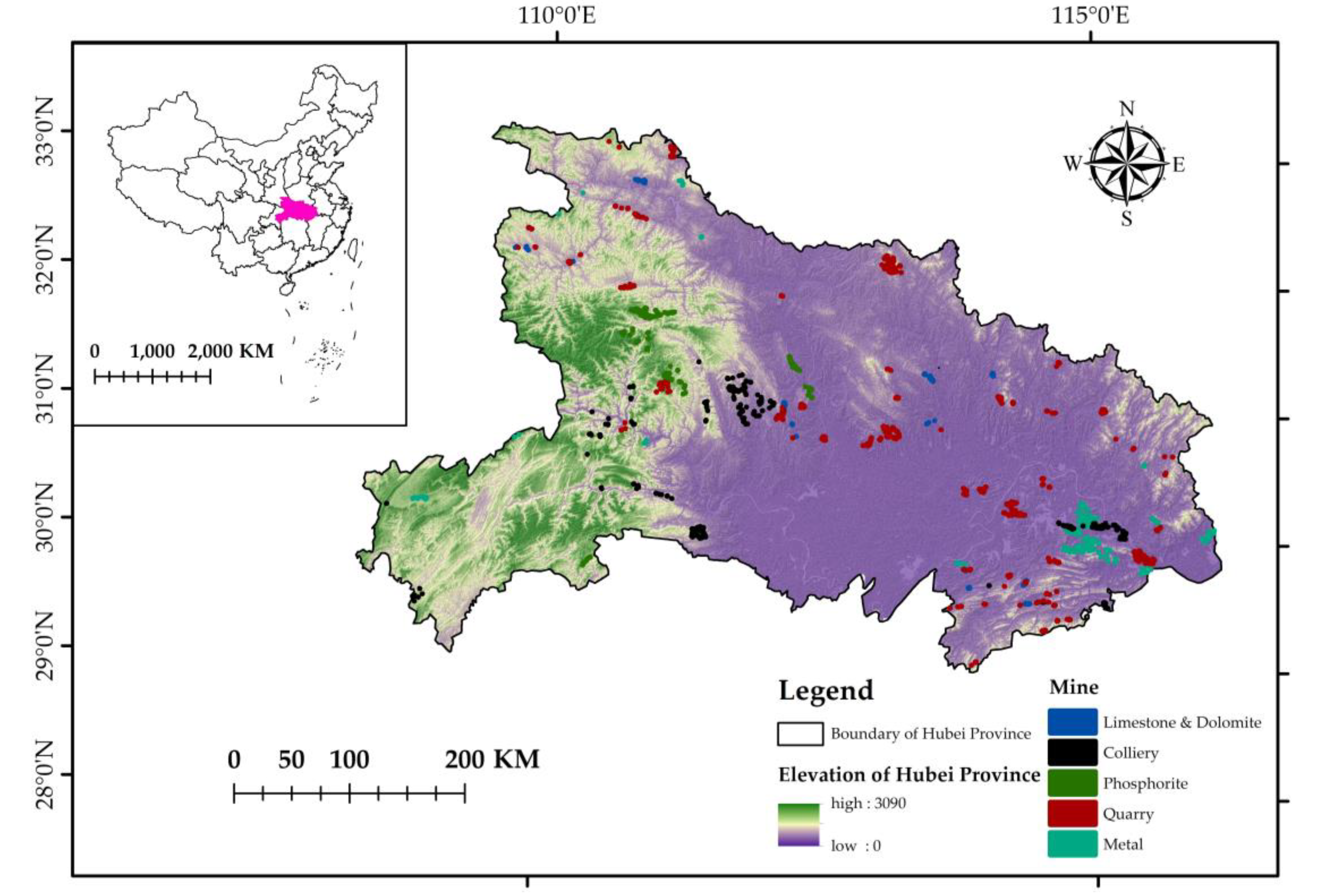
The study area is situated in Hubei Province. Hubei Province is located in central China, and its geographical coordinates are Longitude 108°21′~116°08′ E, Latitude 29°02′~33°17′ N [29]. The topography of the province fluctuates greatly, and the landform is diversified. The whole province spans two first-order tectonic units, the Qinling fold system and the Yangtze paraplatform. Various types of magmatic are widespread, and metamorphic rocks are rich in mineral resources [30]. As shown in Figure 1, the iron, copper, gold and silver deposits in Hubei province are mainly distributed in Proterozoic metamorphic rocks, Mesozoic magmatic rocks and their contact metamorphic zone in Daye, Ezhou, Huangshi, Yangxin, Zhushan and Yunxi. The phosphate mines are located in the Han River alluvial plain and hilly region such as Yicheng and Zhongxiang. Limestone and dolomite mines are distributed in Paleozoic sedimentary strata in Yichang, Wuchang, Jingmen, Xiangfan and Tongshan. Coal and pyrite mines mainly exist in the Paleozoic sedimentary rocks in Yichang, Enshi and Jianshi. The quarries are mainly distributed in Shiyan, Suizhou, Huanggang and other places. The experimental data are all from the key mining areas of remote sensing interpretation in Hubei Province with about 5500 km2, except for Xiantao, Tianmen and Qianjiang.

Figure 1.
Landform and mine distribution map of Hubei Province.
3. Methods
3.1. Improved Mask R-CNN
As the Figure 2 shows, based on the faster R-CNN framework, Mask R-CNN adds a parallel semantic segmentation branch to conduct the target detection and regression [31,32]. In this model, feature pyramid networks (FPN) + ResNet101 is used to extract the features of the backbone network. After feature extraction, this model used the Region Proposal Network (RPN) to carry out end-to-end training of the target detection frame in open-pit mines. The dilated convolution was also involved in the feature calculation and finally used the RoI (Region of Interest) Align to solve the problem of large actual deviation in the original image [33].
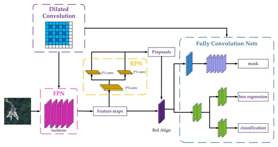
Figure 2.
Mask R-CNN network generalization diagram.
3.1.1. Convolutional Backbone and Dilated Convolution
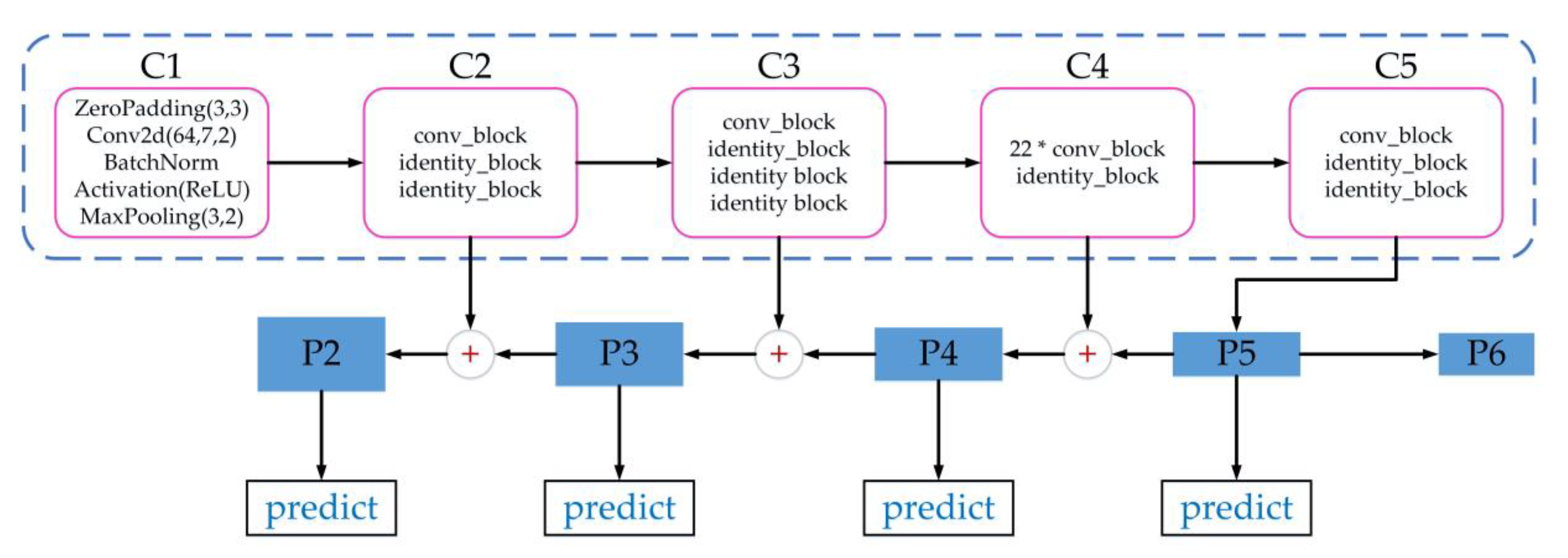
Convolutional backbone is a series feature maps used by convolutional layer to extract open-pit mines, and it mainly applies the structure of ResNet101. The ResNet101 network is a residual network proposed by four scholars from Microsoft Research, and its internal residual block uses skip connects to alleviate the problem of gradient disappearance caused by increasing depth in the network. The deep network is designed as H(x) = F(x) + x, which can also be converted to a residual function F(x) = H(x) − x. As long as F(x) = 0, this formula constitutes an identity map H(x) = x so that the residuals can be fitted more easily [34]. As Figure 3 shows, Mask R-CNN divides the Resnet101 network into five stages, which are denoted as C1, C2, C3, C4, and C5. The five stages correspond to the output of feature maps of five scales, which are used to build the feature pyramid of the FPN network.

Figure 3.
Feature pyramid networks (FPN) structure diagram.
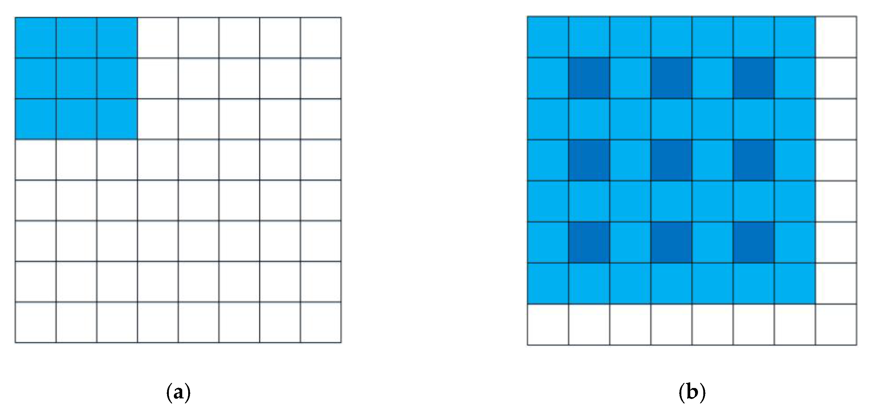
Local receptive fields are a very important concept in the Convolutional Neural Network (CNN). When CNN performs instance segmentation, on account of the final feature map size being much smaller than the size of the input images, the final predicted split mask will be rough. However, the dilated convolution can control the rate of the convolution kernel and obtain different convolution receptive fields [35]. Therefore, dilated convolution solves the contradiction between improving the receptive fields and maintaining the size of the feature map in CNN. Figure 4a shows the local receptive fields with a traditional 3 × 3 convolution kernel, which is the same as the 3 × 3 dilated convolution kernel with a rate of 1. In Figure 4b, when the dilated convolution kernel has a rate of 2, the local receptive field of the convolution kernel increases to 7 × 7. In this paper, a dilated convolution kernel with a rate of 2 is added to the structure of the feature pyramid, and the dilated convolution operation is carried out on the output features in each pyramid stage. Finally, the accuracy of mask prediction can be effectively improved in the category prediction stage at the pixel level.
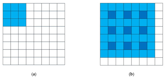
Figure 4.
Local receptive fields: (a) dilated convolution kernel with rate = 1; (b) dilated convolution kernel with rate = 2.
3.1.2. RPN Framework and RoI Align
RPN is a Full Convolutional Neural (FCN) network. RPN carries out an end-to-end training of the open-pit mines target detection frame by adding additional category and regression convolutional layers on the CNN. This framework lays anchor with different proportions on the original image, and, at the same time, it generates candidate boxes which can match the open-pit mines targets of various scales and extract the boundary. RPN first traverses the CNN feature map output with a 3 × 3 sliding window. Mask R-CNN establishes an m × m binary mask to distinguish the front and rear scenes of each target object with the branch of instance segmentation. At the current position in the pixel space of the open-pit mines image, the mapping point of the center sliding window is the anchor [36,37]. Five feature maps, namely, P2, P3, P4, P5, and P6, with different scales are several anchor boxes generated by the RPN, and the preset proposal can obtain the size and coordinates of corresponding areas in the open-pit mines’ target image, where P1, P2, P3, P4, and P5 are the feature pyramid. Mask R-CNN abandons the P1 characteristics of stage1 and takes down sampling based on stage5 (P5) to obtain P6 characteristics. Finally, the five feature maps of different scales (P2, P3, P4, P5, and P6) are input into the RPN to generate RoI, respectively. Due to different stride lengths, RoI Align was performed on the corresponding stride of four feature maps (P2, P3, P4, and P5) with different scales. RoI Align aims to solve the problem of large actual deviation in the original image caused by the formation of candidate regions in the quantization process [38]. Concat connection is conducted based on the RoI Align generated and divides the network into three parts: the fully connected prediction class, the fully connected predictive rectangle box, and the full convolution predicts pixel segmentation. These three parts are represented by the mask, the target border and the border’s class of open-pit mines, respectively.
3.1.3. Border Regression and Loss Function
For a given border (, , , ), target border regression is utilized to obtain the final regression border (, , , ) and make it closer to the real border (, , , ). That is, we need to find a mapping f, such that f(, , , ) = (, , , ), and (, , , ) ≈ (, , , ), where the subscripts x, y, w, and h represent the horizontal distance, the vertical distance, the width and the height of the three types border of center points, respectively. The border regression learns about these transformations, and translation (, ) and scale zooming (, ) are calculated based on the parameters of the real border and the predicted border. The calculations are as follows:
The objective function is expressed as (P) = φ5(P), is the parameter to learn (* represents x, y, w, h), φ5(P) is the eigenvector that predicts the border, and (P) is the regression value obtained. The goal is to minimize the difference between the regression value and the true value = (tx, ty, tw, th). The loss function obtained is as follows:
Discrete probability distribution p is used to represent the probability of the target and background of the open-pit mines, in which the real border is labeled as . The loss function is obtained as follows:
The mean value of the sigmoid function was calculated for each pixel of the mask, which was defined as the average binary cross entropy loss function . This method can effectively improve the effect of instance segmentation. Therefore, the loss function of Mask-RCNN consists of the three loss functions, including classification loss, regression loss and segmentation loss [39]. The total loss function is as follows:
3.2. Transfer Learning
The essence of transfer learning is the transfer and reuse of knowledge. The existing knowledge is called the source domain, while the new knowledge which needs to be learned is called the target domain [40]. According to the definition of transfer learning, it can be divided into three types: distributed differential transfer learning, characteristic differential transfer learning and tag differential transfer learning. Distributed differential transfer learning refers to the difference in the marginal distribution or conditional probability distribution between the source domain and the target domain. Characteristic differential transfer learning refers to the difference in the feature space between the source domain and the target domain. Tag differential transfer learning refers to the difference in the tag space between the source domain and the target domain. Generally, the target domain is different from the source domain in terms of data distribution, characteristic dimensions and model output change conditions [41].
Mathematically, transfer learning contains two elements: domains and tasks [42]. The domains U contains two elements: sample feature space Ӽ and the probability distribution p(x) of the overall x, where the sample set X = () Ӽ, φ. For a domain U = {Ӽ, φ}, we defined the task Г on U as containing two elements: the label space У and the function f, where У is a discrete random variable with uniform distribution. The set Y = () У is the sample of the population, and У is called the label space of Y, where f: Ӽ→У can be obtained from the training sample {}, X,Y. From the view of probability, f can be thought of as the conditional probability p(y|x), and the task can be represented as Г = {У, p(y|x)}. The two tasks are different, if and only if the label space У has at least one difference when compared to conditional probability p(y|x). When the source domain-labeled data . and target domain non-labeled data are fixed, we can finally minimize the binary loss function to improve the learning effect of the target task. In the absence of the target domain calibration data, knowledge transfer can be accomplished by reducing the distribution difference between the source domain and the target domain [43].
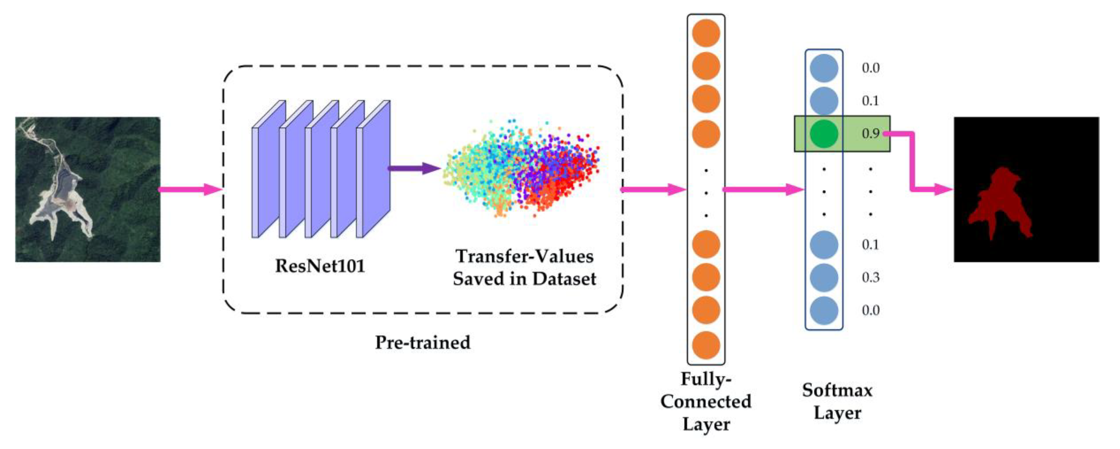
Due to the small number of open-pit mine manual labeling target datasets, the Mask R-CNN network should be pre-trained on the dataset firstly to prevent the model from overfitting. It can be seen that the label space of the source domain (a dataset has already been trained) and target domain (untrained open-pit mines dataset) are different, and the transfer learning of open-pit mines belongs to tag-differential transfer learning. Thus, we must make full use of the Mask R-CNN in the source domain to guide the target recognition of the new open-pit mine dataset [44]. Mask R-CNN has already trained the weights for automatic identification of about 80 categories, such as aircraft and pedestrians. By selecting pre-trained ResNet101 to initialize the model, the transfer values of open-pit mines were saved in a dataset (source domain). As the Figure 5 shows, the pre-trained process generated 1024 features through the fully connected layer, and in the Softmax layer, 80 features were finally generated. On the basis of source domain weight, we used transfer learning to find the category with the closest characteristics of open-pit mines, and the generalization performance of the model was greatly improved.
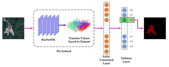
Figure 5.
Transfer learning.
4. Experiments
4.1. Experiment Data
4.1.1. Data Source and Identification Index
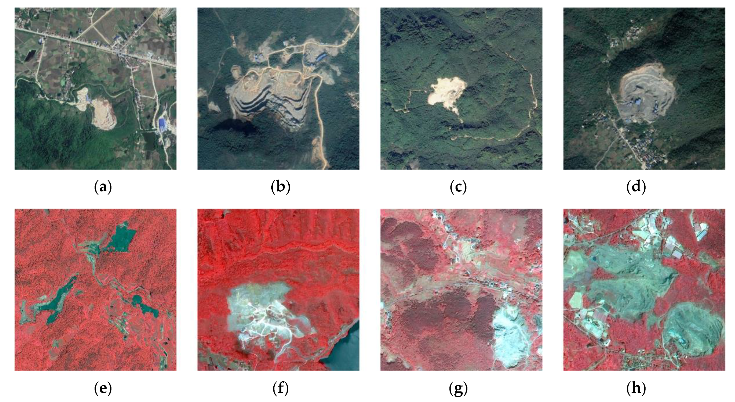
Data sources include image data and auxiliary data. Image data are mainly used for extraction and verification of open-pit mines, while auxiliary data are mainly used to show the spatial distribution characteristics of open-pit mines. We used Gaofen-1 and Gaofen-2 satellite images to monitor the geological environment of open-pit mines, and for areas that were not covered or had unclear images, we supplemented the image data with Google Earth satellite images of the same period. The satellite image data time is from January to August 2019. All the satellite images have been preprocessed by radiometric calibration, atmospheric correction, orthographic correction and image fusion. According to the open-pit mines distribution of mineral resources in Hubei Province, the identification indexes of main open-pit mines are established according to the mining degree and spatial texture characteristics of surface [45]. The interpretation marks established in the open-pit mines were verified by field investigation, and the interpretation signs are summarized as Figure 6.

Figure 6.
Identification index. True-color images: (a) iron mine in Qichun County; (b) quarry mine in Yangxin County; (c) granite mine in Xingshan County; (d) coal mine in Huangshi City; false-color images: (e) coal mine in Yuan’an County; (f) quarry mine in Chibi City; (g) quarry mine in Chongyang County; (h) coal mine in Daye City.
- (1)
- After the rocks and soils are stripped, the surfaces of open-pit mines are mainly steep walls and platforms. The bedrock is bare and fresh, and some of the platforms are piled up with the waste residue. Therefore, the features of open-pit mines in true-color images mainly appear white or yellow, and there are multiple steps or steep slopes connected with roads.
- (2)
- In the false-color image, the difference between the open-pit mines and the images background is obvious. The open-pit mine’s surface is mainly gray or gray-black with a simple texture and regional block, which is in great contrast with the background forest vegetation that a has rough texture and reddish brown reflection.
4.1.2. Sample Database
The sample database of IMRT is mainly divided into user samples and model samples. User samples are mainly extracted from field investigation or visual interpretation of remote sensing images, which are the basis of model samples. Based on the user samples, remote sensing images are converted into a sample format, which is required for the model training and testing through a series of data processing. The experimental source domain data are in the COCO dataset, which has a total of 80 samples with labeled categories. The target domain data are the non-labeled open-pit mines images. The full name of MS COCO is Microsoft Common Objects in Context, which is an object detection and segmentation dataset. The target from complex daily scenes is mainly extracted, and the target of interest can be calibrated by precise segmentation [46,47]. MS COCO uses json files to store the information about target of interest, and it classifies all data into training sets (validation sets are included in the training sets) and test sets. These mainly include object instances, object key points and image captions.
In this paper, the open-pit mine interpretation symbol database was established from the color and texture index of remote sensing images, and on this basis, a training open-pit mine sample dataset of IMRT was made on the structure of the MS COCO classic sample dataset. The experimental data were semantically segmented in the open-pit mines of each image, and the resolution of each image was two meters. The open-pit mine sample dataset mainly adopts the following format: the cv2_mask folder mainly contains all the 8-bit mask labels needed for training; the json folder includes the json file that represents the coordinates of the training object; the labelme_json folder contains the annotation samples for the semantic segmentation of open-pit mines in img.png, info.yaml, label.png, label_names.txt and label_viz.png; and the pic folder mainly contains all the image data in jpg format. The structure is shown in Figure 7.

Figure 7.
Dataset folder of training data.
4.2. Training Environment and Function Analysis
This experiment was conducted in a Windows 64-bit operating system with 16GB running memory. A quad-core Intel CORE I5 9th Gen CPU was configured, and a GeForce GTX 1650TI graphics card was equipped. The running environment of this model is python3.5.6, and the framework is TensorFlow. The training of the IMRT model mainly depends on the libraries, such as TensorFlow, Keras, OpenCV and PIL. TensorFlow uses a data flow diagram to design the computational flow, which enables the users to train large-scale neural networks with parallel operations. Keras is an advanced library for rapidly prototyping deep learning, and it has an excellent expansibility for TensorFlow. PIL mainly obtains the color of the pictures by comparing them with the color library. On the other hand, OpenCV recognizes colors by distinguishing the HSV (Hue, Saturation, Value) components of the picture strictly. These libraries provide a good foundation for us to obtain the low-lever and the high-level features of open-pit mine images better.
The size of sample datasets was set to 600 × 600, and the true-color images (experimental samples) and the false-color images (reference samples) were trained, respectively. The total number of experimental samples is 600, and there were 400 reference samples. The experimental samples and reference samples were trained in batches. With an initial learning rate of 10−3 [48], the network had a total of 100,000 training epochs. During the experiment, the COCO dataset divided all the data into a training set and a test set, among which the validation set is included in the training set.
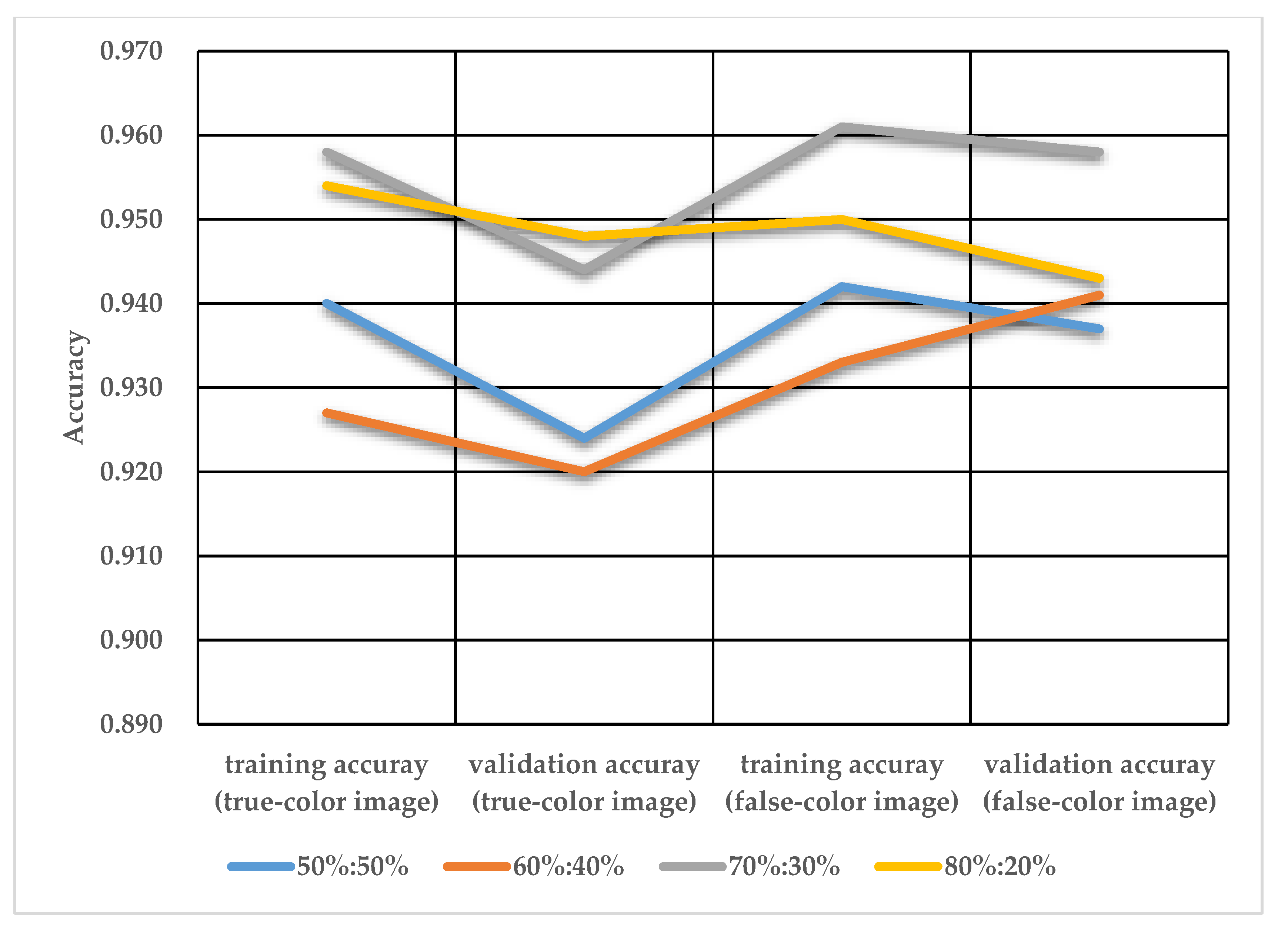
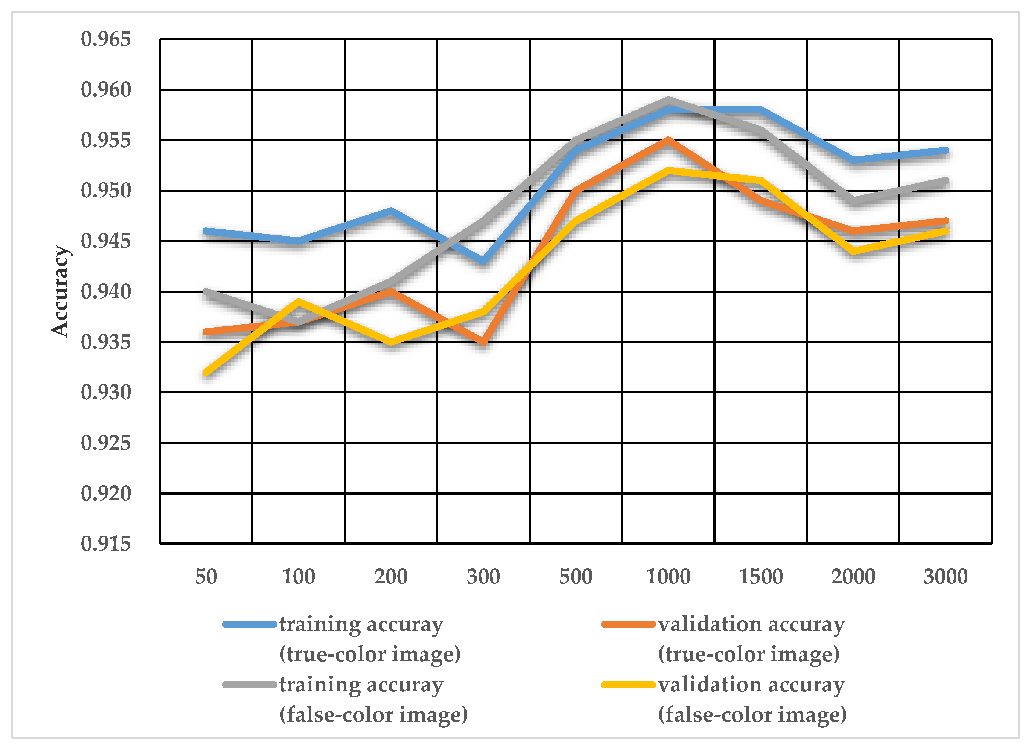
By controlling the constant of batch size, we planned to analyze the accuracy changes in training and validation accuracy by adjusting the ratio of the training set and validation set. After that, we controlled the ratio between the training set and the validation set constant again to obtain the influence of batch size changes on the training and validation accuracy. As shown in Figure 8, the validation accuracy of the true-color image with a ratio of 70%:30% was lower than that with a ratio of 80%:20%, however, the training accuracy of the true-color image as well as the training and validation accuracies of the false-color image were higher than other ratios. When the ratio of the training set and validation set remains unchanged in the process of batch size increasing, the accuracy of the true-color images and false-color images presents an overall trend of increasing and then regional stability. As shown in Figure 9, when the batch size is 1000, there is an advantage. Therefore, the ratio of the training set and validation set is 70%:30%, and the batch size is 1000 to participate in the open-pit mine identification.

Figure 8.
Training and validation accuracies of the true-color image and false-color image under four different ratios of training and validation samples.

Figure 9.
Training and validation accuracies of the true-color image and false-color image under different batch sizes.
4.3. Accuracy Evaluation
The evaluation of open-pit mine extraction accuracy is mainly carried out in two ways: pixel-based evaluation and object-based evaluation. The pixel-based evaluation methods evaluate the extracted pixels and aim to reflect the consistency of the extracted results in geometric accuracy and shape similarity. The object-based evaluation methods can avoid the pixel bias error. With the purpose of analyzing the potential causes of extraction errors, the evaluation results can be correlated with the parameters by quantifying the number of extracted targets. In order to solve the problems such as a fuzzy boundary or complex internal structure, in this paper, we used the two accuracy evaluation methods to evaluate the extraction results.
The evaluation indexes based on pixel are mainly composed of pixel accuracy (PA), comprehensive evaluation index (F1) and Kappa coefficient [49]. PA is an evaluation index to calculate the matching proportion of the predicted pixel values and the real pixel values. The higher the PA, the higher matching degree of the predicted value and the real value. F1 can be regarded as the binary classification problem of open-pit mine targets and backgrounds. Kappa coefficient represents the coincidence degree between the classified image and the reference image, and it is an objective evaluation standard to test their consistency.
where is the number of the correctly classified samples divided by the total number of samples, and is the number of the misclassified samples divided by the total number of samples.
In terms of object-based evaluation, Precision, Recall, FalseAlarm and MissingAlarm [50,51,52] are mainly used to quantitatively evaluate the predicted results. Precision is the ratio between the number of open-pit mines extracted correctly (TP) and the count of the extraction open-pit mines identified by IMRT. Recall is the ratio between the number of open-pit mines and the number of open-pit mines in the sample database. FalseAlarm is the ratio between the number of open-pit mine target identifications wrongly (FP) extracted and the count of the identification results. MissingAlarm is the ratio between the number of omission extractions (FN) and the number of open-pit mines in the sample database.
5. Discussion
5.1. Open-Pit Mine Identification Results
Figure 10 compares the intelligent extraction model with traditional extraction methods of multi-source remote sensing. The extraction results of SVM and MLE have better integrity on the whole, but these traditional extraction methods are mainly affected by the surface objects with high reflectivity, such as bare ground and road, so it is easy for them to be misclassified. Faster R-CNN can locate and classify the target on the spatial position of each open-pit mines accurately, but it lacks the boundary mask information. Compared with the three methods, the IMRT model has better performance in the comprehensive locating boundary precision, the fragmentation degree and the integrity of the extraction boundary of the extraction results. The accuracy evaluation method described above is used to quantify the extraction results of IMRT, faster R-CNN, SVM and MLE models. The pixel-based accuracy evaluation results are shown in Table 1, and the object-based accuracy evaluation results are shown in Table 2. The comparison results are as follows:
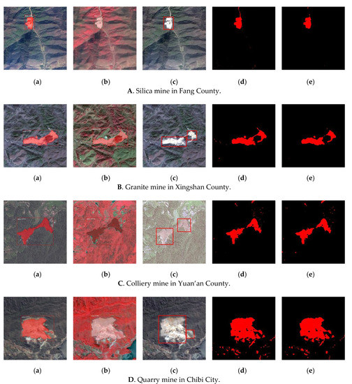
Figure 10.
Mine identification results. (a) Improved Mask R-CNN and Transfer learning (IMRT) identification results of the true-color image; (b) IMRT identification results of the false-color image; (c) faster R-CNN identification results; (d) Maximum Likelihood (MLE) identification results; (e) Support Vector Machine (SVM) identification results.

Table 1.
Precision evaluation based on pixels.

Table 2.
Precision evaluation based on objects.
In true-color images, SVM and MLE extracted the pixels belonging to the supervised classification characteristics of open-pit mines as much as possible, but there were also obvious errors in the extraction results. In Figure 10A, the two traditional extraction methods mistakenly divided the marginal road into an open-pit mine. As shown in Figure 10C, farmland and other land types were classified as open-pit mines. During the influence of spectral characteristics, the open-pit mine extraction of the MLE classification was severely broken and low in accuracy. The extraction results of false-color images by all methods performed well. However, the deep learning model can extract the complete boundary information of block regions. To some extent, the undeveloped areas in the center of open-pit mines also participated in the overall target extraction, so the traditional model performed a little better than the deep learning method, as shown in Figure 10B. Faster R-CNN had a relatively good identification ability for open-pit mines, but for large open-pit mines, the selection area of the identification box was too large. As shown in Figure 10D, when many targets are in the area, it is difficult to truly locate the open-pit mine targets in the image. Compared with the traditional extraction method, the IMRT model was able to extract the complete structures and obvious edge features of small open-pit mines, and it did not cause leakage or misclassification. As shown in Figure 10D, because the false-color image eliminates the influence of water vapor, the extraction effect of open-pit mines with the false-color image is even better than the true-color image. That is to say, the extraction results obtained by IMRT are more consistent with the real surface values.
In terms of pixel-based evaluation, among the two traditional extraction methods, the results of SVM have a better performance, the index of F1 is 0.7148, and the Kappa coefficient is 0.6943, but the PA is slightly lower than that of the MLE, which is 0.9320. For the extraction results of the IMRT model and the faster R-CNN model, the evaluation indexes of the IMRT model are higher than the other one. However, the lowest value of accuracy index in the deep learning method is higher than the highest one of the traditional method, indicating that compared with the traditional method, deep learning has more advantages in open-pit mine recognition. The IMRT model has the best performance in PA and Kappa coefficient, with values of 0.9718 and 0.8251, respectively.
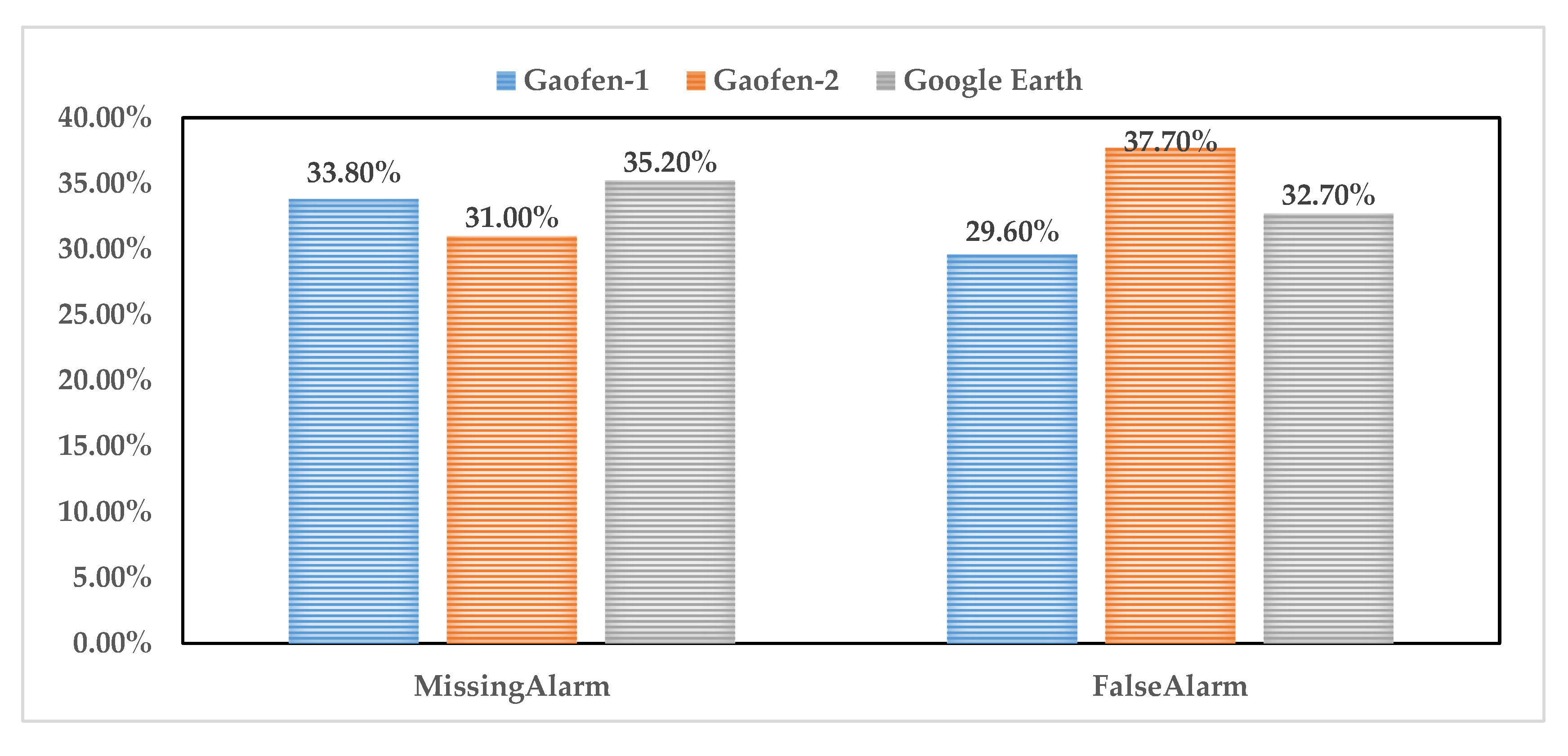
According to object-based evaluation, the Recall and MissingAlarm of MLE classification results are the worst, with values of 0.6826 and 0.3174, respectively, indicating that this method could not identify or classify the open-pit mines well. The FalseAlarm of SVM is the highest, which shows that the error extracted by this method is the biggest. Among the results of IMRT and the faster R-CNN, IMRT has the best Recall and MissingAlarm, with values of 0.9138 and 0.0862. In the index of FalseAlarm, faster R-CNN performs better, at 0.1143, which is a little lower than the IMRT model at 0.0190. Faster R-CNN performs better in terms of FalseAlarm; its value of 0.1143 is slightly lower than that of the IMRT model. Of the three types of satellite image samples statistics (Figure 11), the MissingAlarm of Google Earth satellite images and the FalseAlarm of Gaofen-2 are the highest. However, there is a small difference between the MissingAlarm and the FalseAlarm of the three satellite image samples, which indicates that the IMRT model has good applicability to Gaofen-1, Gaofen-2 and Google Earth satellite images.
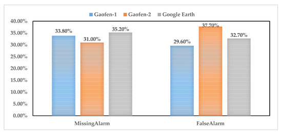
Figure 11.
MissingAlarm and FalseAlarm based on objects.
To sum up, for the multi-source remote sensing image identification of open-pit mines, the deep learning identification method is better than the traditional target identification method in precision and effect. To be specific, the Precision, F1 and FalseAlarm of the faster R-CNN model are the best, and IMRT is better in PA, Kappa coefficient, Recall and MissingAlarm, which shows that both the IMRT model and the faster R-CNN deep learning model have a good effect on the target identification of open-pit mines. Compared with faster R-CNN, IMRT has a better performance on MissingAlarm, which proves that this model has a higher accuracy of identification. Thus, IMRT is more suitable for the identification of open-pit mines with multi-source remote sensing images.
5.2. Open-Pit Mine Dynamic Monitoring
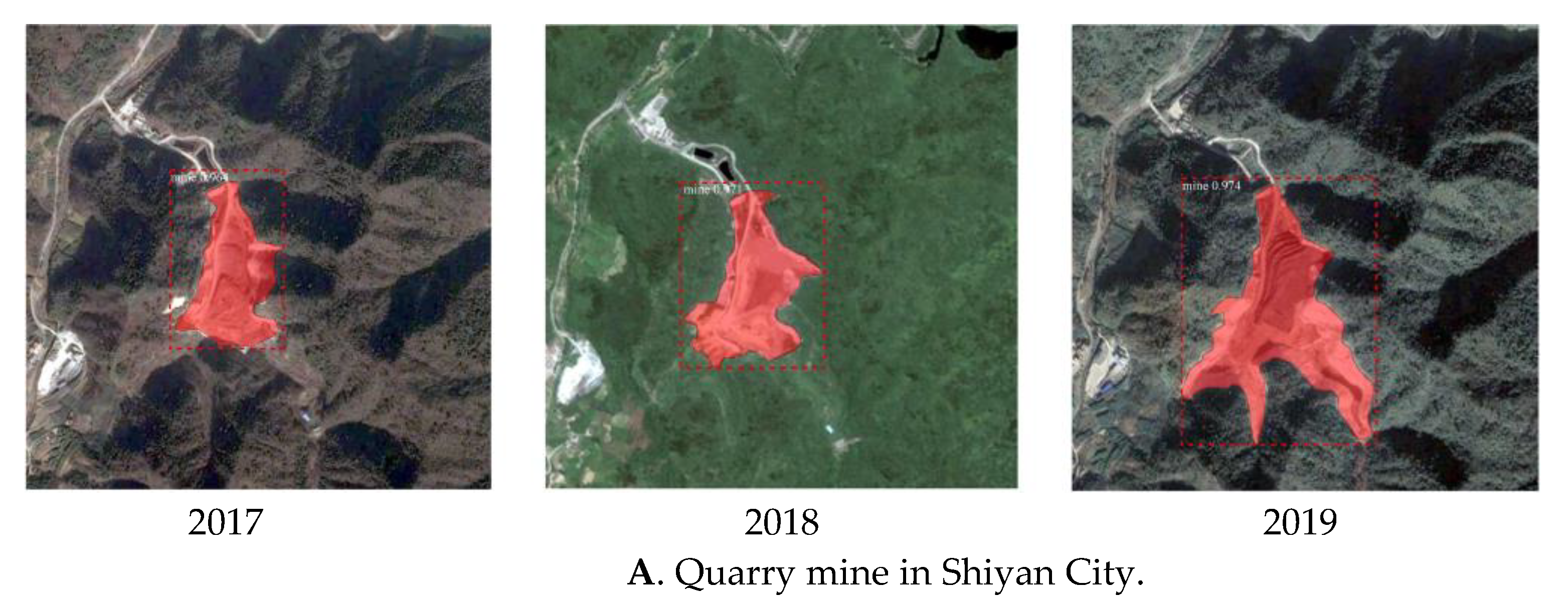
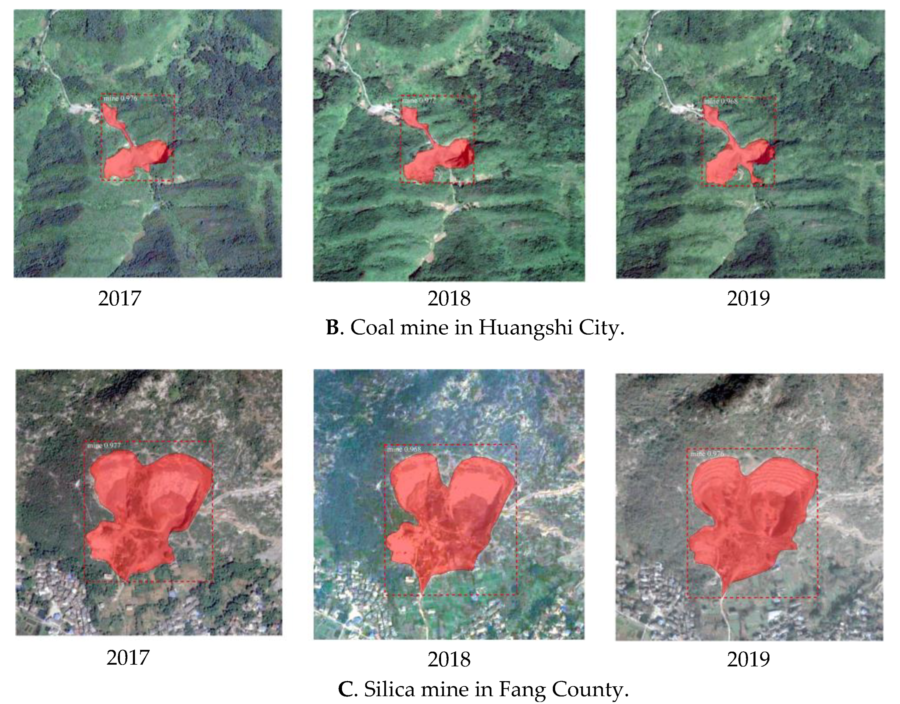
The remote sensing interpretation results of Hubei Province show that there are open-pit mines in the key mining areas of the whole province. Among which, the open-pit mines in western, northern, central and eastern of Hubei Province are relatively concentrated, and the central region is comparatively sparse. There are 25 key mining areas in Yichang, thus representing the area with the most mines in Hubei Province, followed by Xianning and Huangshi. According to the comprehensive interpretation of key mining areas in each city, Huangshi has the largest number of open-pit mines. Jingmen and Shiyan have the most abundant interpretation types, and, on the contrary, Huanggang, Jingzhou and Shennongjia have the least. Based on the Geological Environment Monitoring Report of 130 Key Mining Areas in Hubei Province and the target identification results of IMRT for open-pit mine during 2017–2019, there were 1213 open-pit mines in 2017, 1179 in 2018, and 1114 in 2019. As is shown in Figure 12, in the three-year dynamic monitoring, the number of open-pit mines decreases year by year, while the area of the majority open-pit mines continues to increase. For example, the quarry mine in Shiyan City, the coal mine in Huangshi City and the silica mine in Fang County have been continuously expanding in the past three years. The monitoring results in this paper show that the target boundary of the open-pit mines is continuously expanding. The target recognition study based on the IMRT model has promoted the application of automatic extraction in open-pit mines.
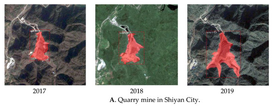

Figure 12.
Open-pit mine changes from 2017 to 2019.
5.3. Assessment of Mine Environment Damages
The characteristics and intensity of mines’ geological environment problems are closely related to mines’ geological environment background and topographical landscape damages. Therefore, the damages rate of the topographical landscape (DROTL) is an important index to demonstrate the influence of mines’ geological environments. In this paper, three levels are used to evaluate the impact degree of topographical landscapes. Level I represents the DROTL when it is above 40%; level II represents the DROTL when it is between 20% and 40%; and level III represents the DROTL when it is less than 20%. The evaluation formula is as follows:
where is the topographical landscape damaged area and is the open-pit mining area.
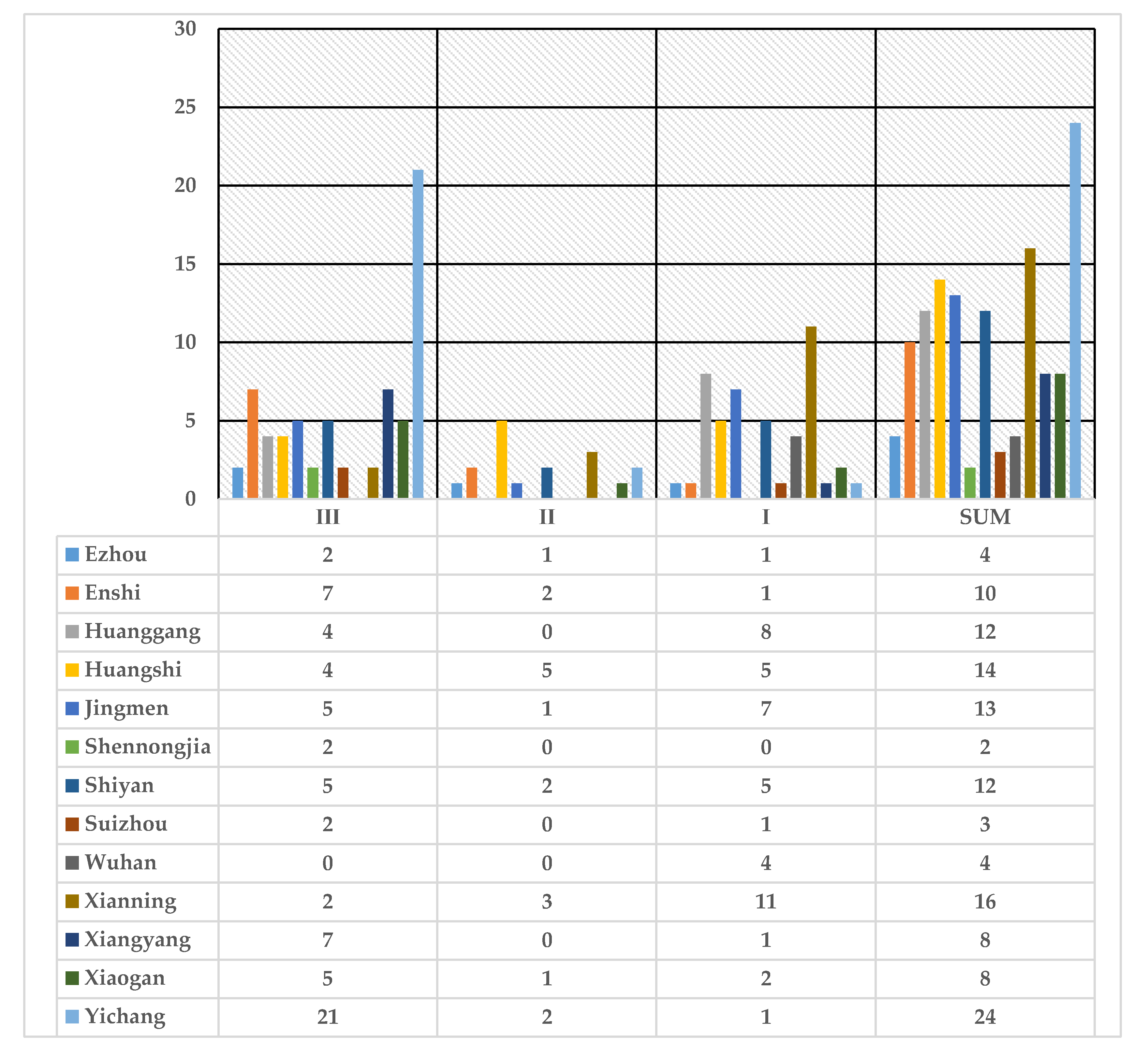
The damages of topographical landscape are evaluated with the recognition results of IMRT and the remote sensing interpretation results. As shown in Figure 13, the total number of key mining areas in Shennongjia is two, representing the smallest number. As we can see, the DROTL level of all the key mining areas is Ⅲ, showing that the damage degree of this area is relatively slight. The maximum number of key mining area is 24 in Yichang, and the DROTL levels are mostly Ⅲ, with only 1 for level I. This indicates that the mines in this region are in reasonable exploitation. The topographical landscapes in Huangshi, Xianning and Jingmen are seriously damaged, and with 75.0%, 68.8% and 53.8% of the topographical landscape destruction in their regions, respectively, they are represented by level I. A total of 36.2% of topographical landscape damage to the key mining area reached level I in Hubei Province, which shows that mineral exploitation has caused serious damage to the topographical landscape.
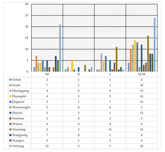
Figure 13.
The damages rate of the topographical landscape of cities in Hubei.
In the remote sensing interpretation of mines’ geological environments, the level of land occupation and destruction (Table 3) is mainly evaluated through the degree of occupation and destruction of farmland, forest land (or grassland) and unused land. As shown in Table 4, in the evaluation, there are 45 key mining areas in level I, 37 key mining areas in level II, 44 key mining areas in level III, and 4 key mining areas without mining land occupation or destruction. Level I of land occupation and destruction represents a total of 34.62%, which is close to the amount of key mining areas facing topographical landscape damage.

Table 3.
The scale of land occupation and destruction evaluation.

Table 4.
The level of land occupation and destruction of cities in Hubei.
Large-scale and high-intensity development of mines directly lead to geological environment problems such as destruction of water resource balance and reduction of vegetation coverage and land occupation. It is necessary for departments to exercise their functions, regulate the mineral resource exploitation activities and ensure the orderly exploitation of mineral resources. Through mine monitoring, it is of great practical significance to provide accurate and reliable data for departments and realize the coordinated development of mines and the ecological environment.
6. Conclusions
Deep learning provides an approach to learn effective features automatically from a training set, and it can perform unsupervised characteristic learning from an enormous original image dataset. In view of the low extraction accuracy, low efficiency and low degree of automation of remote sensing images of mines by traditional methods, we proposed an open-pit mine extraction model bases on Improved Mask R-CNN and Transfer learning (IMRT), constructed a set of multi-source mine sample databases consisting of Gaofen-1, Gaofen-2 and Google Earth satellite images with a resolution of two meters, and designed an automatic batch production process of open-pit mine targets in order to automatically identify and dynamically monitor open-pit mines. The main conclusions are as follows:
- (1)
- The experiment results show that the IMRT model is superior to traditional methods in precision, generalization, automation and efficiency. At the same time, this model has a good applicability for Gaofen-1, Gaofen-2 and Google Earth satellite images, which expands the data source of open-pit mines and enhances the practicability of model.
- (2)
- Remote sensing images are used to identify the open-pit mines in Hubei Province from 2017 to 2019 automatically. By analyzing the target recognition results of IMRT, it is shown that although the number of open-pit mines is slowly decreasing, some of the key mining areas are increasing. Part of the open-pit mines is constantly expanding.
- (3)
- Level I (serious) of land occupation and destruction accounts for 34.62%, and 36.2% of topographical landscape damage reached level I, which shows that the mineral exploitation has caused serious damage to the topographical landscape. It is necessary for the departments to regulate mineral resource exploitation activities and ensure the orderly exploitation of mineral resources.
Author Contributions
Conceptualization, C.W.; methodology, C.W. and L.C.; software, C.W. and L.C.; validation, C.W.; formal analysis, C.W., L.C. and L.Z.; resources, R.N.; writing—original draft, C.W.; writing—review and editing, C.W. and L.Z. All authors have read and agreed to the published version of the manuscript.
Funding
This research received no external funding.
Acknowledgments
This work is funded by Hubei Geological Environment Station. The vector data of 130 key mines in Hubei Province as well as Gaofen-1 and Gaofen-2 satellite images are mainly provided by the Hubei Data and Application Center.
Conflicts of Interest
The authors declare no conflict of interest.
References
- Pohl, C.; van Genderen, J. Multisensor image fusion in remote sensing: Concepts, methods and applications. Int. J. Remote Sens. 1998, 19, 823–854. [Google Scholar] [CrossRef]
- Ji, S.; Tian, S.; Zhang, C. Urban Land Cover Classification and Change Detection Using Fully Atrous Convolutional Neural Network. Geomat. Inf. Sci. Wuhan Univ. 2020, 45, 233–241. [Google Scholar]
- Zainuddin, M.; Kiyofuji, H.; Saitoh, K.; Saitoh, S. Using multi-sensor satellite remote sensing and catch data to detect ocean hot spots for albacore (Thunnus alalunga) in the northwestern North Pacific. Deep-Sea Res. Part II 2006, 53, 419–431. [Google Scholar] [CrossRef]
- Xiao, W.; Zhang, W.; Lyu, X.; Wang, X. Spatio-temporal patterns of ecological capital under different mining intensities in an ecologically fragile mining area in Western China: A case study of Shenfu mining area. J. Nat. Res. 2020, 35, 68–81. [Google Scholar]
- Wang, L.; Jin, X.; Jia, H.; Tang, Y.; Ma, G. Change detection for mine environment based on domestic high resolution satellite images. Remote Sens. Land Resour. 2018, 30, 151–158. [Google Scholar]
- Nguyen, A.; Liou, Y.; Li, M.; Tran, T. Zoning eco-environmental vulnerability for environmental management and protection. Ecol. Indic. 2016, 69, 100–117. [Google Scholar] [CrossRef]
- Asif, Z.; Chen, Z. An integrated optimization and simulation approach for air pollution control under uncertainty in open-pit metal mine. Front. Environ. Sci. Eng. 2019, 13, 2095–2201. [Google Scholar] [CrossRef]
- He, F.; Xu, Y.; Chen, H.; Zhang, J. Present status of mine geohazards in the northwest region of China and characteristics of their temporal-spatial distribution. Geol. Bull. China 2008, 27, 1245–1255. [Google Scholar]
- Gong, P.; Liu, H.; Zhang, M.; Li, C.; Wang, J. Stable classification with limited sample: Transferring a 30-m resolution sample set collected in 2015 to mapping 10-m resolution global land cover in 2017. Sci. Bull. 2019, 64, 370–373. [Google Scholar] [CrossRef]
- Diao, M.; Liu, F.; Tan, Z.; Xue, T.; Wang, Y. Research and implement on automatic production method of mine remote sensing monitoring interpretation record table. Remote Sens. Land Resour. 2018, 30, 212–217. [Google Scholar]
- Alborzi, N.; Poorahangaryan, F.; Beheshti, H. Spectral-spatial Classification of Hyperspectral Images Using Signal Subspace Identification and Edge-preserving Filter. Int. J. Autom. Comput. 2020, 17, 222–232. [Google Scholar] [CrossRef]
- Huang, X.; Zhang, L.; Li, P. Classification of High Spatial Resolution Remotely Sensed Imagery Based Upon Fusion of Multiscale Features and SVM. J. Remote Sens. 2007, 11, 48–54. [Google Scholar]
- Hou, W.; Lu, X.; Zhang, C.; Wang, J. Object-oriented Information Extraction from High Resolution Imagery: A Case Study for Recognition of Residential Area in Lixian County, Sichuan Province. J. Geo-Inf. Sci. 2010, 12, 119–125. [Google Scholar]
- Kang, J.; Zhou, L.; Zhao, D.; Wen, X. High Resolution Remote Sensing Image Object Recognition Method Based on Histogram Feature Knowledge Base. Chin. Rare Earth 2020, 41, 32–40. [Google Scholar]
- Sampath, A.K.; Gomathi, N. Decision tree and deep learning based probabilistic model for character recognition. J. Cent. South Univ. 2017, 24, 2862–2876. [Google Scholar] [CrossRef]
- Yu, K.; Jia, L.; Chen, Y.; Xu, W. Deep Learning: Yesterday, Today, and Tomorrow. J. Comput. Resour. Dev. 2013, 50, 1799–1804. [Google Scholar]
- Dang, Y.; Zhang, J.; Deng, K.; Zhao, Y.; Yu, F. Study on the Evaluation of Land Cover Classification using Remote Sensing Images Based on AlexNet. J. Geo-Inf. Sci. 2017, 19, 1530–1537. [Google Scholar]
- Wang, L.; Li, J.; Zhou, G.; Yang, D. Application of Deep Transfer Learning in Hyperspectral Image Classification. Comput. Eng. A 2019, 55, 181–186. [Google Scholar]
- Clabaut, É.; Lemelin, M.; Germain, M.; Williamson, M.; Brassard, É. A Deep Learning Approach to the Detection of Gossans in the Canadian Arctic. Remote Sens. 2020, 12, 3123. [Google Scholar] [CrossRef]
- Cai, H.; Xu, Y.; Li, Z.; Cao, H.; Feng, Y.; Chen, S.; Li, Y. The division of metallogenic prospective areas based on convolutional neural network model: A case study of the Daqiao gold polymetallic deposit. Geol. Bull. China 2019, 38, 1999–2009. [Google Scholar]
- Yang, H.; Zhao, Y.; Dong, J. Remote sensing image super-resolution of open-pit mining area based on texture transfer. J. China Coal Soc. 2019, 44, 3781–3789. [Google Scholar]
- Xiang, Y.; Zhao, Y.; Dong, J. Remote sensing image mining area change detection based on improved UNet siamese network. J. China Coal Soc. 2019, 44, 3773–3780. [Google Scholar]
- Wu, Z.; Lei, S.; Lu, Q.; Bian, Z.; Ge, S. Spatial distribution of the impact of surface mining on the landscape ecological health of semi-arid grasslands. Ecol. Indic. 2020, 111, 105996. [Google Scholar] [CrossRef]
- Slavomir, L.; Marcela, B.; Zofia, K.; Stefan, K.; Gabriel, F.; Vieroslav, M. Utilization of Geodetic Methods Results in Small Open-Pit Mine Conditions: A Case Study from Slovakia. Minerals 2020, 10, 489–510. [Google Scholar]
- Gong, C.; Lei, S.; Bian, Z.; Liu, Y.; Zhang, Z.; Cheng, W. Analysis of the Development of an Erosion Gully in an Open-Pit Coal Mine Dump During a Winter Freeze-Thaw Cycle by Using Low-Cost UAVs. Remote Sens. 2019, 11, 1365. [Google Scholar] [CrossRef]
- Zhang, Y.; Shen, W.; Li, M.; Lv, Y. Integrating Landsat Time Series Observations and Corona Images to Characterize Forest Change Patterns in a Mining Region of Nanjing, Eastern China from 1967 to 2019. Remote Sens. 2020, 12, 3191. [Google Scholar] [CrossRef]
- Wen, Y.; Li, L.; Shang, X.; Hu, F. An Instance Segmentation Method based on Improved MASK RCNN Feature Fusion. Comput. A Softw. 2019, 36, 130–133. [Google Scholar]
- Lu, H.; Fu, X.; He, Y.; Li, L.; Zhuang, W.; Liu, T. Cultivated Land Information Extraction from High Resolution UAV Images Based on Transfer Learning. Trans. Chin. Soc. Agric. Mach. 2015, 46, 274–279, 284. [Google Scholar]
- Wang, S.; Zhang, Z.; Zhao, X.; Zhou, Q. Eco-environmental synthetic analysis based on RS and GIS technology in Hubei province. Adv. Earth Sci. 2002, 17, 426–431. [Google Scholar]
- Zhou, T.; Fan, Y.; Yuan, F. Advances on petrogensis and metallogeny study of the mineralization belt of the Middle and Lower Reaches of the Yangtze River area. Acta. Petrol. Sin. 2008, 24, 1665–1678. [Google Scholar]
- Zhang, W.; Witharana, C.; Liljedahl, A.K.; Kanevskiy, M. Deep Convolutional Neural Networks for Automated Characterization of Arctic Ice-Wedge Polygons in Very High Spatial Resolution Aerial Imagery. Remote Sens. 2018, 10, 1487. [Google Scholar] [CrossRef]
- Kalfarisi, R.; Wu, Z.; Soh, K. Crack Detection and Segmentation Using Deep Learning with 3D Reality Mesh Model for Quantitative Assessment and Integrated Visualization. J. Comput. Civil. Eng. 2020, 34, 04020010. [Google Scholar] [CrossRef]
- Machefer, M.; Lemarchand, F.; Bonnefond, V.; Hitchins, A.; Sidiropoulos, P. Mask R-CNN Refitting Strategy for Plant Counting and Sizing in UAV Imagery. Remote Sens. 2020, 12, 3015. [Google Scholar] [CrossRef]
- Schaap, M.; Leij, F.; van Genuchten, M. Neural network analysis for hierarchical prediction of soil hydraulic properties. Soil Sci. Soc. Am. J. 1998, 62, 847–855. [Google Scholar] [CrossRef]
- Panboonyuen, T.; Jitkajornwanich, K.; Lawawirojwong, S.; Srestasathiern, P.; Vateekul, P. Semantic Labeling in Remote Sensing Corpora Using Feature Fusion-Based Enhanced Global Convolutional Network with High-Resolution Representations and Depthwise Atrous Convolution. Remote Sens. 2020, 11, 1233. [Google Scholar] [CrossRef]
- Sizkouhi, A.; Aghaei, M.; Esmailifar, S.; Mohammadi, M.; Grimaccia, F. Automatic Boundary Extraction of Large-Scale Photovoltaic Plants Using a Fully Convolutional Network on Aerial Imagery. IEEE J. Photovolt. 2020, 10, 1061–1067. [Google Scholar] [CrossRef]
- Almubarak, H.; Bazi, Y.; Alajlan, N. Two-Stage Mask-RCNN Approach for Detecting and Segmenting the Optic Nerve Head, Optic Disc, and Optic Cup in Fundus Images. Appl. Sci. 2020, 10, 3833. [Google Scholar] [CrossRef]
- Li, D.; He, W.; Guo, B.; Li, M.; Chen, M. Building target detection algorithm based on Mask-RCNN. Sci. Surv. Mapp. 2019, 44, 172–180. [Google Scholar]
- Shi, J.; Zhou, Y.; Zhang, Q. Service robot item recognition system based on improved Mask RCNN and Kinect. Chin. J. Sci. Instrum. 2019, 40, 216–228. [Google Scholar]
- Zhuang, F.; Luo, P.; He, Q.; Shi, Z. Survey on Transfer Learning Research. J. Softw. 2015, 26, 26–39. [Google Scholar]
- Hu, F.; Xia, G.; Hu, J.; Zhang, L. Transferring Deep Convolutional Neural Networks for the Scene Classification of High-Resolution Remote Sensing Imagery. Remote Sens. 2015, 7, 14680–14707. [Google Scholar] [CrossRef]
- Zhang, B.; Shi, Z.; Zhao, X.; Zhang, J. A Transfer Learning Based on Canonical Correlation Analysis Across Different Domains. Chin. J. Comput. 2015, 38, 1326–1336. [Google Scholar]
- Zlateski, A.; Jaroensri, R.; Sharma, P.; Durand, F. On the Importance of Label Quality for Semantic Segmentation. In Proceedings of the IEEE/CVF Conference on Computer Vision and Pattern Recognition, Salt Lake City, UT, USA, 18–22 June 2018; pp. 1479–1487. [Google Scholar]
- Wu, T.; Luo, J.; Xia, L.; Yang, H.; Shen, Z.; Hu, X. An Automatic Sample Collection Method for Object-oriented Classification of Remotely Sensed Imageries Based on Transfer Learning. Acta Geol. Cartogr. Sin. 2014, 43, 908–916. [Google Scholar]
- Li, C.; Lu, L.; Bi, M.; Wang, M.; Zhao, G. Sythetic information ore-prospecting model for gold minerals of Baishan area, Jilin. World Geol. 2010, 29, 71–77. [Google Scholar]
- Vinyals, O.; Toshev, A.; Bengio, S.; Erhan, D. Show and Tell: Lessons Learned from the 2015 MSCOCO Image Captioning Challenge. IEEE Trans. Pattern Anal. 2017, 39, 652–663. [Google Scholar] [CrossRef]
- Xu, C.; Wang, X.; Yang, Y. Attention-YOLO: YOLO Detection Algorithm That Introduces Attention Mechanism. Comput. Eng. A. 2019, 55, 13–23, 125. [Google Scholar]
- Lv, Y.; Zhang, C.; Yun, W.; Gao, L.; Wang, H.; Ma, J.; Li, H.; Zhu, D. The Delineation and Grading of Actual Crop Production Units in Modern Smallholder Areas Using RS Data and Mask R-CNN. Remote Sens. 2020, 12, 1074. [Google Scholar] [CrossRef]
- Song, X.; Jiao, L. Classification of Hyperspectral Remote Sensing Image Based on Sparse Representation and Spectral Information. J. Electron. Inf. Technol. 2012, 34, 268–272. [Google Scholar]
- Li, Q.; Liu, X.; Li, M.; Niu, J.; Li, R. A target detection algorithm of HFSWR based on redundant discrete wavelet transform. Chin. J. Radio Sci. 2016, 31, 501–507. [Google Scholar]
- Duan, R.; Zhao, W.; Huang, S.; Chen, J. Fast line detection algorithm based on improved Hough transformation. Chin. J. Sci. Instrum. 2010, 31, 2774–2780. [Google Scholar]
- Lin, Y.; Zhang, B.; Xu, J.; Hou, K.; Zhou, X. Building Extraction from High Resolution Remote Sensing Imagery with Multi-feature and Multi-scale. Bull. Surv. Mapp. 2017, 12, 53–57. [Google Scholar]
Publisher’s Note: MDPI stays neutral with regard to jurisdictional claims in published maps and institutional affiliations. |
© 2020 by the authors. Licensee MDPI, Basel, Switzerland. This article is an open access article distributed under the terms and conditions of the Creative Commons Attribution (CC BY) license (http://creativecommons.org/licenses/by/4.0/).

