Abstract
The Gravity Recovery and Climate Experiment (GRACE) mission has provided global observations of temporal variations in the gravity field resulting from mass redistribution at the surface and within the Earth for the period 2002–2017. Although GRACE satellites are not able to realistically detect the second zonal parameter (ΔC20) of geopotential associated with the flattening of the Earth, they can accurately determine variations in degree-2 order-1 (ΔC21, ΔS21) coefficients that are proportional to variations in polar motion. Therefore, GRACE measurements are commonly exploited to interpret polar motion changes due to variations in the global mass redistribution, especially in the continental hydrosphere and cryosphere. Such impacts are usually examined by computing the so-called hydrological polar motion excitation (HAM) and cryospheric polar motion excitation (CAM), often analyzed together as HAM/CAM. The great success of the GRACE mission and the scientific robustness of its data contributed to the launch of its successor, GRACE Follow-On (GRACE-FO), which began in May 2018 and continues to the present. This study presents the first estimates of HAM/CAM computed from GRACE-FO data provided by three data centers: Center for Space Research (CSR), Jet Propulsion Laboratory (JPL), and GeoForschungsZentrum (GFZ). In this paper, the data series is computed using different types of GRACE/GRACE-FO data: ΔC21, ΔS21 coefficients of geopotential, gridded terrestrial water storage anomalies, and mascon solutions. We compare and evaluate different methods of HAM/CAM estimation and examine the compatibility between CSR, JPL, and GFZ data. We also validate different HAM/CAM estimations using precise geodetic measurements and geophysical models. Analysis of data from the first 19 months of GRACE-FO shows that the consistency between GRACE-FO-based HAM/CAM and observed hydrological/cryospheric signals in polar motion is similar to the consistency obtained for the initial period of the GRACE mission, worse than the consistency received for the best GRACE period, and higher than the consistency obtained for the terminal phase of the GRACE mission. In general, the current quality of HAM/CAM from GRACE Follow-On meets expectations. In the following months, after full calibration of the instruments, this accuracy is expected to increase.
1. Introduction
1.1. Polar Motion Variations due to Mass Redistribution
The Earth’s gravity field is changing in time and space because of mass displacements in the surficial fluid layers: the atmosphere, the ocean, the land hydrosphere. Such mass variability induces variations in Earth orientation parameters (EOPs): precession and nutation, polar motion (PM), and length-of-day (LOD) variations [1]. The EOPs should be determined with the highest possible accuracy, because they have many applications in modern geodesy, astronomy, and other disciplines. Such applications include transforming coordinates from a terrestrial reference frame into a celestial reference frame, precise positioning of objects on the Earth’s surface, launching and navigating spacecraft and satellites.
PM variations result from many geophysical processes, which are characterized by different frequencies, from a few days to decades [2]. Among these factors we can distinguish mass redistribution of atmosphere, oceans, continental water, snow and ice, the gravitational attraction of the Sun, Moon, and planets, interactions between core and mantle [3], or even climate changes [4,5]. However, over the last few decades, researchers have focused mainly on interpretation of changes in PM caused by global and regional mass redistribution [6,7,8,9,10,11,12]. Such impacts have been proven to be the main contributors to variation in the Earth’s rotation for time scales of a few years or less, especially for seasonal time scales [13,14].
The excitation of PM resulting from changing mass redistribution of Earth surficial fluid layers is usually represented with effective angular momentum (EAM) functions: atmospheric, oceanic, hydrological, and cryospheric (called atmospheric angular momentum (AAM), oceanic angular momentum (OAM), hydrological angular momentum (HAM), and cryospheric angular momentum (CAM), respectively). However, the author of work [15] argued that it is difficult to separate cryospheric signals, especially those from mountain glaciers. This is because of the small spatial scales of mountain glaciers, difficulties in the separation of mountain glacier mass signals from surrounding hydrological signals, and absence of data over some mountain glacier regions in models of glacial isostatic adjustment (GIA) [15]. Therefore, HAM and CAM are usually treated together to reflect the total effect of water stored in soil moisture, groundwater, surface water, snow, ice, and biomass. In many papers [6,7,9,10,11], such excitation is denoted as HAM, even though it represents the impact of not only liquid water but also snow and ice. Therefore, to emphasize that we consider effects from all water storage components, including continental water, snow and ice, we use HAM/CAM instead of HAM in the remainder of this paper.
PM variations are described in terms of the two equatorial components of excitation function of the Earth rotation. The first of them, χ1, is oriented towards the Prime (Greenwich) Meridian, and the second one, χ2, is perpendicular to χ1 and oriented towards 90° E. The complex form of the equatorial components (χ1 + iχ2) is also used. The axial component (χ3) of the excitation function of the Earth rotation is related to LOD variations. The spatial distribution of the main continents and oceans leads to a situation in which χ2 is more closely related to the mass redistribution on land in the Northern Hemisphere, whereas χ1 is more sensitive to mass changes over the Greenland Ice Sheet and oceans.
In general, the contribution of geophysical impacts to the PM variation is investigated by studying the geophysical excitation, which describes the influence of the sum of the atmospheric, oceanic, and hydrological/cryospheric effects (AAM + OAM + HAM/CAM). Nevertheless, other phenomena, which are hard to detect and measure, also contribute to the geophysical excitation (for example the effects from earthquakes). From the geodetic perspective, the total PM excitation resulting from external factors can be measured. Contemporary space geodesy and satellite techniques, including Satellite Laser Ranging (SLR), Global Navigation Satellite Systems (GNSS), and Very Long Baseline Interferometry (VLBI) deliver accurate and precise observations of EOPs. For example, the current accuracy of PM measurements is as high as 0.05 mas (miliarcseconds) (1 mas is about 3 cm on the surface of Earth). The geodetic angular momentum (GAM), or geodetic excitation of PM, describes the full variation of PM resulting from all external impacts. Equatorial components (χ1, χ2) of GAM are obtained from precisely measured coordinates (x, y) of the pole, using Liouville’s equation [16,17]. In an ideal situation, if all geophysical processes were to be considered during the determination of geophysical excitation, and no errors were related with geodetic measurements, the geodetic excitation and geophysical excitation would be the same. However, they are not equal because of the presence of both observation errors and model errors. Moreover, some geophysical phenomena, that are currently difficult to detect or measure, are omitted.
PM changes due to angular momentum have been studied in the last few decades based on geophysical models and observations of the atmosphere and oceans [1,6,18,19,20,21,22,23,24]. The knowledge of atmospheric pressure and wind fields enable the computation of AAM, while ocean bottom pressure and ocean currents are essential for the calculation of OAM. It has previously been demonstrated that at seasonal and subseasonal time scales, the sum of AAM and OAM explain 80% of PM excitation [19,21]. The residual variation can be associated with HAM/CAM, which describes mass changes in land hydrosphere constituents, such as soil water, surface water, groundwater, snow water, ice, and water in biomass. The sum of these components is usually called the terrestrial water storage (TWS). However, although the role of AAM and OAM in the PM excitation budget has been well known and described, the HAM/CAM causes the biggest part of uncertainty. This problem is not so visible in the case of LOD and precession and nutation, because HAM/CAM has a smaller impact on these EOPs. Precession and nutation are also well established by theoretical models.
1.2. Hydrological/Cryospheric Excitation of PM from Hydrological and Climate Models
In many studies, HAM/CAM has been estimated using meteorological measurements, numerical climate models, or global hydrological models [6,7,9,11,25,26,27,28,29,30,31]. Hydrological models are usually obtained from ground-based and satellite observations and simulations of the distribution of various TWS components (soil water, surface water, canopy water storage, etc.) [32]. The climate models are more complex as they integrate different modules (land hydrosphere constituents, ocean, atmosphere, ice) to analyze climate evolution and predict its future changes resulting from e.g., increasing of CO2 concentration in the atmosphere [33]. The authors of [25] showed that variations in the land hydrosphere are the main contributors to PM excitation at seasonal time scales because of the strong seasonal cycle in the continental water storage. However, HAM/CAM obtained from different model data exhibit visible divergences, which include differences between particular model estimates and discrepancies between model estimates and the hydrological/cryospheric signals in observed PM excitation [6,9,11,28,29,30]. Currently available global water storage models suffer from many limitations, such as the lack of a groundwater storage component, lack of adequately modelled polar ice sheets, or ignoring global mass conservation [34]. The sources of differences between particular hydrological and climate models include differences in processing algorithms, input data, number of parameters estimated, and spatial and temporal resolution. In our previous works [9,10,11,12,28,29], we compared and evaluated HAM/CAM obtained from several hydrological and climate models. In particular, in [11] we tested various hydrological models from the Global Land Data Assimilation System (GLDAS), in [9] we evaluated GLDAS, the Land Surface Discharge Model (LSDM), and several climate models from the CMIP5 (Coupled Model Intercomparison Project Phase 5), in [10,12] we validated LSDM in different spectral bands. In work [29] the Climate Prediction Center (CPC) model, National Oceanic and Atmospheric Administration (NOAA) model, GLDAS, and LSDM were compared with gravimetric and geodetic observations, while in paper [28] a validation of the National Center for Environmental Prediction/National Center for Atmospheric Research (NCEP/NCAR) model, WaterGAP Global Hydrology Model (WGHM), GLDAS, CPC, and NOAA was presented. However, all those works underlined that HAM/CAM obtained from hydrological and climate models are in worse consistency with observed hydrological/cryospheric signals than HAM/CAM computed from gravimetric observations provided by the Gravity Recovery and Climate Experiment (GRACE) mission.
1.3. Hydrological/Cryospheric Excitation of PM from GRACE and GRACE-FO
Alternative sources of data for the determination of PM excitation due to global mass variations are observations of Earth gravity field changes. Such unique data has been delivered by the GRACE mission [35,36,37,38]. In the years 2002–2017, two GRACE twin satellites measured mutually the changes in distance between them, which allowed changes in the Earth’s gravity field to be determined, resulting from variations in the redistribution of surface fluids. The changes in the Earth’s gravitational field as measured by GRACE are usually represented by monthly gravity field models consisting of spherical harmonics (SH) coefficients of geopotential. Although GRACE satellites are not able to realistically detect the second zonal parameter (ΔC20) of geopotential that is related to the Earth’s oblateness, they can precisely determine variations in degree-2 order-1 (ΔC21, ΔS21) coefficients that are proportional to changes in PM. Therefore, GRACE measurements are commonly exploited to interpret polar motion variations due to changes in global mass redistribution, especially in the continental hydrosphere and cryosphere. After the removal of tidal contributions and nontidal atmospheric and oceanic effects from the GRACE-based gravity fields, the residual signal mostly indicate the land hydrosphere and cryosphere contribution. Therefore, the use of Earth’s gravity field variations due to changes in land water, snow, and ice mass represents another approach to assess the hydrological/cryospheric excitation of PM independently from geophysical models. GRACE temporal gravity field estimates have been used in a number of studies to determine mass-related hydrological/cryospheric PM excitation (e.g., [8,9,10,11,12,39,40,41,42]). It was generally concluded that global observations of the Earth’s gravity field variations by GRACE provide hydrological/cryospheric excitation of PM with higher accuracy than hydrological models [9,11,12]. There has also been an attempt to exploit global gravity models based on kinematic orbits of low-Earth-orbit satellites other than GRACE, such as Swarm, TerraSAR-X, TanDEM-X, MetOp-A, MetOp-B, and Jason 2 [43]. However, the accuracy of the determined HAM/CAM was found to be less satisfactory than that derived from GRACE estimates [43].
During the entire 15-year period of the GRACE activity, the quality of its measurements was not equal and this was mainly due to equipment deterioration. In particular, in the terminal phase of the GRACE, which is after 2016, the data noise increased noticeably as a result of a change in thermal control of the spacecraft due to the increasingly limited battery capacity. A further decrease in the accuracy of the GRACE data in 2017 was due to exclusion of one of the two accelerometers. However, in the initial phase of the mission, the measurements were also not free from the impact of equipment condition, as the proper calibration of all instruments took time. The GRACE data analyses showed that the best GRACE performance occurred in the years 2006–2013 [12].
The unprecedented success and scientific robustness of the data from the GRACE mission, which terminated in 2017, contributed to the launch of its successor, GRACE Follow-On (GRACE-FO or GFO) [44]. The goal of the GRACE-FO, which began in May 2018, was to continue high-resolution global measurements of temporal variations in the Earth’s gravity field. The orbit and design of the GRACE-FO constellation is similar to the satellite system of its predecessor. As in the previous mission, in GRACE-FO, two twin satellites are placed in the same, almost polar (inclination 89°) low Earth orbit (altitude of ~500 km), at a distance of about 220 km from each other. The two satellites use a dedicated two-way microwave ranging system to precisely measure changes in the distance and speed between them, which can be then used to determine the Earth’s gravity field variations and global mass changes. Despite its similar design to GRACE, GRACE-FO incorporates a number of improvements, such as a laser-ranging interferometer (LRI), which, together with a K-band microwave system, is used to measure the distance between satellites. LRI enables even more accurate inter-satellite ranging because of the shorter wavelength of light. Another update is the use of three star cameras instead of two to improve the orientation of the satellites.
The monthly time series of both GRACE- and GRACE-FO-based geopotential models are made available to users by official GRACE/GRACE-FO data centers at GeoForschungsZentrum (GFZ) in Potsdam, Germany; the Jet Propulsion Laboratory (JPL) in Pasadena, CA, USA; and the Center for Space Research (CSR) in Austin, TX, USA.
The objective of the current study is to present the first estimates of HAM/CAM obtained from the new GRACE-FO mission. The novelty in this work is also that the three different GRACE/GRACE-FO data types are used to calculate, compare, and evaluate HAM/CAM: (1) ΔC21, ΔS21 coefficients of geopotential (GRACE/GRACE-FO Level-2 data), also named as GSM coefficients; (2) gridded TWS anomalies (GRACE/GRACE-FO Level-3 data); and (3) mascon (MAS) solutions (GRACE/GRACE-FO Level-3 data). We also confront and validate various methods of HAM/CAM estimation and discuss the reasons for the differences between HAM/CAM calculated using these methods. The study of the consistency between the solutions from CSR, JPL, and GFZ is included as well. We also evaluate different HAM/CAM series using precise geodetic measurements of the pole coordinates and geophysical models of AAM and OAM. Based on comparison with HAM/CAM data obtained from the previous GRACE mission, we attempt to assess the updates and improvements in hydrology/cryosphere-related excitation of PM. The analyses are divided into three parts: (1) internal consistency of GRACE- and GRACE-FO-based HAM/CAM; (2) external validation of GRACE- and GRACE-FO-based HAM/CAM conducted by comparing HAM/CAM with the hydrological signal in observed PM excitation (geodetic residuals (GAO)); and (3) comparison of consistency between GAO and HAM/CAM based on GSM coefficients, gridded TWS anomalies, and mascon data. These analyses can be useful in determining the accuracy of measurements of the new GRACE-FO mission, especially in the context of using them to interpret changes in PM.
2. Materials and Methods
2.1. HAM/CAM from Different GRACE and GRACE-FO Data Types
The GRACE/GRACE-FO Level-2 data are commonly used in the determination of HAM/CAM. The datasets have the form of spherical harmonics (SH) coefficients of geopotential, also known as Stokes’ coefficients or GSM (GRACE/GRACE-FO satellite-only model). The variations of χ1 and χ2 equatorial components of HAM/CAM depend on variations of degree-2, order-1 spherical harmonic coefficients (ΔC21, ΔS21) of geopotential models (based on [17,45]):
where Re is the Earth’s mean radius; M is the Earth’s mass; A, B, and C are the principal moments of inertia for Earth; A’ = (A + B)/2 is an average of the equatorial principal moments of inertia and A = 8.0101 × 1037 kg·m2, B = 8.0103 × 1037 kg·m2, and C = 8.0365 × 1037 kg·m2 (Table 1 in [45]); and ΔC21 and ΔS21 are the normalized spherical harmonics coefficients of the gravity field.
HAM/CAM series obtained in this way mainly indicate the impact of the land hydrosphere and cryosphere. However, GIA, barystatic sea-level contributions resulting from inflow of water from land into oceans (so-called sea-level angular momentum or SLAM), and earthquake signatures are not removed. In addition, some residual signals from ocean (signals from residual variations remaining over the ocean after removing the appropriate ocean model, partly related to ocean model errors and leakage between land and ocean) might be also retained. However, it should be noted that both atmospheric and oceanic signals are removed from all GRACE data products using Atmosphere and Ocean De-aliasing (AOD) data. In particular, AOD data removes ocean dynamic effects from GRACE gravity fields. The residual ocean signals retained in HAM/CAM computed from GSM may be due to the non-removal of the entire mass of oceans, errors in the ocean model used to determine AOD, and leakage between land and ocean. Therefore, in this paper, we refer to these signals as residual ocean signals. Since the χ2 component of HAM/CAM is more closely related to mass variations over lands, the unremoved signals from the oceans should not affect noticeably the variability of this component. However, they can affect χ1 component, because it is associated with ΔC21 representing much part of the oceans. It should also be kept in mind that, similar to GSM-based HAM/CAM, in GAO, which is the reference for evaluating HAM/CAM, GIA is not removed. GIA apply to the readjustment in response to the last deglaciation, but also to present ice mass changes. Therefore, it is important to consider GIA, especially in the case of Greenland that has been distinguished by significant mass loss in recent years. However, GIA affects mainly trend in PM excitation and do not affect the seasonal or short-term variability of HAM/CAM. GIA impact can be eliminated using a GIA model such as ICE6G model [46] or model developed by A et al. [47]. Barystatic sea-level changes, signals from earthquakes, and atmosphere and ocean model errors are associated with both GAO and GRACE/GRACE-FO-based HAM/CAM.
Another method of determining HAM/CAM from GRACE/GRACE-FO is to exploit TWS anomalies (GRACE/GRACE-FO Level-3 data). In this method, equatorial components of HAM/CAM (χ1, χ2) are calculated by summing up the impacts of TWS (Δq) over the whole Earth [17]:
where is a change in TWS; are latitude, longitude, and time, respectively; Re is Earth’s mean radius; dS is the surface area; and C and A are Earth’s principal moments of inertia. The factor 1.098 accounts for the yielding of the solid Earth to surface load, rotational deformation, and core–mantle decoupling [17].
To compute HAM/CAM using this method, 2 different GRACE/GRACE-FO data types can be used, first, TWS anomalies given in regular grids and obtained from SH coefficients, and second, TWS anomalies computed using mascon (MAS) approach.
In the first data set, TWS anomalies are given in regular latitude-longitude grids and are obtained from SH coefficients of all available degrees and orders, after appropriate reprocessing (filtering, correcting due to GIA, replacing ΔC20 coefficient with an estimate from SLR, and correcting degree-1 coefficients). These products provide information on changes in the water content in terrestrial areas only because of the masking of ocean regions. Consequently, the resulting HAM/CAM series describe the effects from continental water, snow and ice without residual ocean signals, or barystatic sea-level changes. However, due to the truncation of spherical harmonics and filtration of TWS solutions, some parts of real geophysical signal are removed. Therefore, to restore these removed signals, the scaling factors are applied to the data [48].
The use of a mascon (MAS) approach for determining TWS anomalies involves directly using the inter-satellite range-rate and acceleration observation to estimate the mass changes of mass concentration blocks on the Earth’s surface [49,50,51]. Like gridded TWS anomalies, MAS represents GRACE/GRACE-FO Level-3 data, delivering monthly changes of TWS. However, in contrast to SH-based TWS anomalies, MAS-based TWS anomalies are given in blocks with known geophysical locations [51,52]. Unlike GSM data and gridded TWS anomalies, MAS models do not use spherical harmonic functions but instead apply mass concentration functions. There are several classes of MAS solutions but usually, MAS-based TWS anomalies are computed directly from inter-satellite range-rate measurements through explicit partial derivatives. This approach leads to GRACE/GRACE-FO maps without north–south stripes, and consequently, there is no need to use filtering, which has been known to remove some real geophysical signals along with the stripes. The GIA, ΔC20, degree-1 coefficient corrections used in gridded TWS anomalies are also applied in MAS solutions. The MAS approach also enables better separation of land and ocean signals than SH approach. HAM/CAM series obtained from MAS data only express the impact of land hydrosphere, snow, and ice on PM excitation because it masks the ocean areas. It should be noted that for both TWS and MAS data considered here, the same GIA model was applied [46], so the consistency between these types of data is conserved. Note that ΔC20, degree-1, and GIA corrections applied in Level-3 data are not implemented in Level-2 data.
The methods of data processing in the newest realization of GRACE models (Release-06 or RL06) and first GRACE-FO series were consistent, including the use of the same background models (e.g., model of static gravity field, planetary ephemerides, mean pole model, and ocean tides model) and the same dealiasing product (Atmosphere and Ocean De-Aliasing Level-1B Release-6 or AOD1B RL06). For both GRACE and GRACE-FO, the same 3 data types (GSM, TWS, and MAS) are developed and made available to the users. The data file formats also remain the same The PM excitation caused by land hydrosphere and cryosphere and obtained from the GRACE/GRACE-FO observations is denoted in previous studies as gravimetric–hydrological excitation, gravimetric excitation, or simply GRACE-/GRACE-FO-based HAM (or HAM/CAM).
In this study, for Level-2 GRACE/GRACE-FO data, we used 3 monthly GSM solutions provided by the 3 official data centers:
- Jet Propulsion Laboratory (JPL), Pasadena, CA, USA—JPL RL06 solution;
- Center for Space Research (CSR), Austin, TX, USA—CSR RL06 solution;
- GeoForschungsZentrum (GFZ) Potsdam, Germany—GFZ RL06 solution.
For Level-3 GRACE/GRACE-FO data, we used 3 monthly TWS solutions (obtained from spherical harmonics of all available degrees and orders) provided by the same 3 data centers (JPL RL06, CSR RL06 and GFZ RL06 solutions) and 1 MAS solution provided by JPL (JPL RL06M v02 solution). All the data were obtained from JPL PO.DAAC Drive (https://podaac-tools.jpl.nasa.gov/drive/files/GeodeticsGravity). The spatial sampling of TWS solutions used in this study was 1°, while the spatial sampling of MAS data exploited here was 0.5°. However, the sampling does not reflect real spatial resolution of GRACE/ GRACE-FO datasets, because it depends on many factors, including filtering, leakage errors, or scaling factors used. Nevertheless, to keep consistency between TWS and MAS data, we downsampled MAS solution into regular 1° latitude-longitude grids using 3D linear interpolation. However, HAM/CAM obtained for downsampled and nondownsampled MAS data presented the same geophysical effect on polar motion.
It should be noted that there are other institutes that process and distribute temporal gravity models, including the Institute of Geodesy at Graz University of Technology (ITSG) in Graz, Austria; the Centre National d’Études Spatiales (CNES) in Toulouse, France; and Tongji University in Shanghai, China. However, to date, only CSR, JPL, and GFZ provide GRACE and GRACE-FO solutions for both Level-2 and Level-3 data, so in this study we focused on data from these 3 institutes. The GRACE data covered the time period between April 2002 and June 2017, while, at the time of this study, GRACE-FO series were available for June 2018 to December 2019, which was selected as the study period. Each GRACE and GRACE-FO time series had a monthly temporal resolution. In the following, for HAM/CAM computed from ΔC21, ΔS21, we use “GSM-based HAM/CAM”, for HAM/CAM computed from TWS anomalies based on spherical harmonics, we use “TWS-based HAM/CAM”, and for HAM/CAM computed from TWS anomalies taken from MAS, we use “MAS-based HAM/CAM”.
2.2. Observed Hydrological Signal in PM Excitation
A common way of evaluating model-based HAM/CAM or GRACE/GRACE-FO-based HAM/CAM series is to compare them with the hydrological/cryospheric signals in the observed excitation. Such signal can be computed from precise measurements of pole coordinates and models of geophysical processes occurring in the atmosphere and the ocean. In order to separate hydrological and cryospheric effects from observed geodetic excitation (geodetic angular momentum or GAM), the signals from atmosphere and ocean are removed from the GAM series to obtain the residual series, named geodetic residuals (GAM–AAM–OAM or GAO), according to the formula:
where GAM is geodetic angular momentum, AAM is atmospheric angular momentum, and OAM is oceanic angular momentum. AAM and OAM are also denoted as the effective angular momentum functions (EAMF) of atmosphere and ocean.
GAO = GAM − AAM − OAM,
In Equation (5), GAM is computed from precise coordinates of the pole, whereas AAM and OAM are based on geophysical models of atmosphere and ocean. In GAO, both mass terms (related to atmospheric air pressure and ocean bottom pressure) and motion terms (related to wind speed and ocean currents) are removed. It is important, because GRACE and GRACE-FO satellites are able to measure changes in mass but they cannot detect mass movement. Removing mass and motion terms of AAM and OAM from GAM makes GAO consistent with HAM/CAM from GRACE/ GRACE-FO. Nevertheless, it is of common knowledge that motion components of AAM and OAM are much weaker than corresponding mass terms [19,45,53]. The resulting GAO series represents mainly the impact of land hydrosphere and cryosphere on PM excitation, but also contains signals from GIA, barystatic sea-level changes, and large earthquakes. They do not contain signals from atmosphere and oceans.
In this study, the χ1 and χ2 equatorial components of GAM were based on daily combined EOP 14 C04 series derived from VLBI, SLR, and GNSS [54], which can be accessed from the International Earth Rotation and Reference System Service (IERS) website (https://www.iers.org/IERS/EN/DataProducts/EarthOrientationData/eop.html, accessed on 20 April 2020). The series are available at temporal resolution of 24 h and are updated regularly. Here, in order to calculate GAM, we used the algorithm provided by Ch. Bizouard, which is available at http://hpiers.obspm.fr/eop-pc/index.php?index=excitactive&lang=en (accessed on 20 April 2020).
For AAM, we used χ1 and χ2 mass and motion series based on the ECMWF (European Center for Medium-Range Weather Forecasts) model [14]. For OAM, we used the χ1 and χ2 mass and motion series based on MPIOM (Max Planck Institute Ocean Model) [55]. Both AAM and OAM series are available at http://rz-vm115.gfz-potsdam.de:8080/repository (accessed on 20 April 2020) and have temporal resolution of 3 h. The data sets were provided by GFZ and they are called ESM (Earth System Model) GFZ data.
Our motivation for choosing ESM GFZ series was that they are consistent with Atmosphere and Ocean De-Aliasing Level-1B Release-6 (AOD1B RL06) data [56], used in the processing of GRACE and GRACE-FO gravity fields. Both AOD1B RL06 and ESM GFZ use the same models of atmosphere and ocean (ECMWF and MPIOM, respectively). Therefore, GAO series computed using AAM and OAM time series from GFZ provide results comparable with GRACE/GRACE-FO estimates. Of course, the GAO series used for evaluation of GRACE/GRACE-FO HAM/CAM are not free of errors. In particular, they are affected by uncertainties in the atmospheric and oceanic models. However, in our previous work [9], we showed that the choice of AAM and OAM models does not affect the level of correlation between GAO and HAM/CAM. Nevertheless, it can have some influence on the amplitudes of GAO.
It should be kept in mind that GRACE/GRACE-FO estimates have a temporal resolution of 1 month, the GAM has a temporal resolution of 24 h, while AAM and OAM have a resolution of 3 h. Therefore, in order to maintain consistency between all datasets, we removed oscillations with periods shorter than 1 month from the GAM, AAM, and OAM series by downsampling them through the application of a Gaussian filter with full width at half maximum (FWHM) equal to 60 days.
3. Results
In the first part of this study, we focus on analysis of internal agreement between HAM/CAM obtained from different GRACE and GRACE-FO solutions. To do this, we analyze the differences among HAM/CAM series from different GRACE models and we assess the deviation from the mean (Section 3.1). We then perform an external validation of GRACE/GRACE-FO-based HAM/CAM series based on comparison with GAO data (Section 3.2). Finally, in the last section (Section 3.3) we focus on comparing HAM/CAM series obtained from the three GRACE/GRACE-FO data types (GSM, TWS, and MAS) from one data center and contrast them with the GAO data.
3.1. Internal Consistency of GRACE- and GRACE-FO-Based HAM/CAM Estimates
At present, a number of temporal gravity models based on GRACE/GRACE-FO observations are available to users (available e.g., at http://icgem.gfz-potsdam.de/series). These estimates, made accessible by various institutes, have different processing strategies, parameters, and background models applied. Therefore, the results arising from their use are similar but not identical. The differences between particular GRACE/GRACE-FO models make the interpretation of the results more difficult. The question of which solution is the most appropriate remains unanswered because the response depends on, among other factors, the purpose of the intended research. Previous papers that have exploited temporal gravity models to analyze global mass changes or PM variations due to mass redistribution used either the data from one processing center (e.g., [30,41,57]) or the mean of several solutions (e.g., [11,58]). There are also papers in which a number of GRACE models were evaluated based on external data (e.g., [9,10,12,40,42]), but no detailed compatibility analysis between individual GRACE solutions was performed. In particular, no such analysis has been conducted for the newest generation of the GRACE models (RL06) or for the first GRACE-FO datasets. Therefore, we begin our analyses with a study of the internal consistency between HAM/CAM from GRACE/GRACE-FO solutions.
It should be noted that most of the previous papers that evaluated PM excitation series computed from GRACE gravity models used either GSM coefficients or TWS gridded data, but there have been few attempts to compare these two methods. An attempt to do so was undertaken by our group [9,59], but this was performed for the previous release of GRACE models (RL05). Similarly, the authors of [8] examined the consistency of the previous GRACE RL05 and GRACE RL06 solutions in the form of TWS and geopotential coefficients. Therefore, here, we perform such an analysis for both the latest generation of the GRACE series (RL06) and the first GRACE-FO estimates.
For an analysis of consistency between GRACE/GRACE-FO solutions, we selected HAM/CAM series obtained from two data types (GSM and TWS), as the MAS solution was not available for all three data centers. The series are presented in Figure 1. For completeness, the series of GAO are also plotted in Figure 1, but they are discussed in detail in Section 3.2. Discussion of trends in HAM/CAM and GAO is also included in the next section. It is clear from Figure 1 that GRACE/GRACE-FO-based HAM/CAM series are more consistent with each other when Level-3 TWS data are used. In addition, TWS-based HAM/CAM data are also characterized by smaller amplitudes than GSM-based HAM/CAM. The smaller amplitudes of TWS-based HAM/CAM can result from the fact that all residual ocean signals, which were not removed during GRACE/GRACE-FO data processing, are eliminated here using land mask. However, in GSM-based HAM/CAM such signals are not removed entirely. GSM-based HAM/CAM includes contributions from not only land hydrosphere and cryosphere, but also some ocean mass which is passively determined by TWS, because the use of AOD1B removes only ocean dynamic effect. This proves that non-removal of the residual signals from the ocean can have an impact on lower consistency between HAM/CAM series obtained from different data centers. This is particularly true for χ1, because this component is more sensitive to mass changes over oceans.
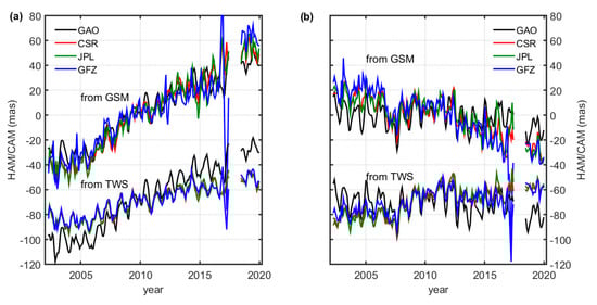
Figure 1.
Time series of (a) χ1 and (b) χ2 components of hydrological polar motion excitation and cryospheric polar motion excitation (HAM/CAM) computed from the Gravity Recovery and Climate Experiment (GRACE) and GRACE Follow-On (GRACE-FO) monthly solutions from official GRACE/GRACE-FO processing centers at Center for Space Research (CSR), Jet Propulsion Laboratory (JPL), and GeoForschungsZentrum (GFZ). Level-2 data (GSM) and Level-3 data (terrestrial water storage (TWS)) are considered. Time series for geodetic residuals (GAO) are added for comparison. The offset value between ΔC21, ΔS21 coefficients of geopotential (GRACE/GRACE-FO Level-2 data (GSM)-based HAM/CAM and TWS-based HAM/CAM time series, used for better data visibility, is 70 mas.
Some conclusions about the uncertainties of GSM-based HAM/CAM can be drawn from Figure 2, which presents the errors of HAM/CAM computed from formal errors of the ΔC21 and ΔS21 coefficients. Mean errors and standard deviation (STD) of errors are also added for each time series. However, it should be kept in mind that the levels of formal errors of the coefficients do not result from validation using external data. They rather reflect the quality of the algorithm used. Nevertheless, the values can be helpful in assessing improvements in the GRACE-FO processing strategy compared with its predecessor. It is clear from Figure 2 that the best performance of the GRACE mission is found for the period between 2006 and 2013, which was also noted in other works [12,60]. During this period, all the instruments on board the GRACE satellites were working properly and had not yet degraded. Compared with data from other processing centers, the CSR series provides the lowest errors of HAM/CAM, which may prove the best quality of the CSR data processing algorithm. The errors of GRACE-FO-based HAM/CAM are visibly lower and more constant than errors obtained for GRACE estimates, which indicates that the GRACE-FO mission performs better in its initial phase than the GRACE mission in the same phase. The errors of TWS-based HAM/CAM are not presented here because the errors of TWS gridded data are not publicly available. However, it should be kept in mind that such errors would be complex, because the TWS estimation requires the use of coefficients of all available degrees, and it is known that as the degree increases, the results become more noisy and the errors rise. Moreover, GRACE/GRACE-FO Level-3 data uncertainties also depend on the filter applied, gain factors used to restore the signal lost during filtration, and errors of the GIA model applied. These uncertainties are not applicable to Level-2 data, which does not apply these processing steps.
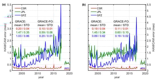
Figure 2.
Errors of χ1 (a) and χ2 (b) components of HAM/CAM obtained from GRACE Level-2 data. The errors were computed from formal errors of ΔC21, ΔS21 coefficients. Mean errors and STD of errors are added for each time series.
In order to check consistency among GRACE and GRACE-FO data, we present root mean square (RMS) of the differences (or root mean square errors, RMSE) between HAM/CAM calculated from particular GRACE and GRACE-FO solutions separately for GSM and TWS estimates (Table 1a). The results are supplemented with correlation coefficients between HAM/CAM series (also Table 1a). As shown in Table 1a, the lowest RMSE and the highest correlations are obtained when GRACE/GRACE-FO data from CSR and JPL are compared (correlation coefficients are above 0.80 for both GRACE and GRACE-FO; RMSE values vary from 1.71 to 5.42 mas for GRACE and from 1.00 to 3.34 mas for GRACE-FO). Similar conclusions were drawn in our previous paper [12], where we compared GSM-based HAM/CAM computed from data provided by different data centers. GRACE/GRACE-FO-based HAM/CAM series are the most compatible with each other when TWS data are used, which may be due to the masking of all residual ocean signals in these series. It is also apparent that HAM/CAM series from particular GRACE/GRACE-FO solutions are more compatible for χ2 than for χ1 because of the spatial distribution of main continents and the fact that χ2 is more responsible to mass changes over lands than χ1. Therefore, a better HAM/CAM quality is expected for χ2. The consistency between HAM/CAM from particular solutions is higher for GRACE-FO than for GRACE (lower RMSE, higher correlations); however, it should be kept in mind that GRACE-FO series are currently shorter than GRACE series and this might affect the quality assessment of GRACE-FO-based HAM/CAM estimates.

Table 1.
(a) Root mean square (RMS) of differences (root-mean-square errors, RMSE) and correlation coefficients between HAM/CAM from particular GRACE/GRACE-FO solutions and (b) RMSE between HAM/CAM from particular GRACE/GRACE-FO solutions and HAM/CAM from mean GRACE/GRACE-FO (mean of CSR, JPL, and GFZ solutions). Note that for GRACE, the critical value of correlation coefficient for 58 independent points and a 95% confidence level is 0.22, while the standard error of the difference between two correlation coefficients is 0.19. For GRACE-FO, the critical value of correlation coefficient for 12 independent points and a 95% confidence level is 0.50, while the standard error of the difference between two correlation coefficients is 0.47.
We now analyze particular HAM/CAM series by checking their deviation from the mean. To do this, we show RMSE and correlation coefficients between HAM/CAM obtained from particular GRACE/GRACE-FO data and HAM/CAM from mean GRACE/GRACE-FO (mean of data from CSR, JPL, and GFZ) (Table 1b). As it can be seen from Table 1b, the GRACE/GRACE-FO-based HAM/CAM series are more consistent with the mean when the Level-3 datasets are used, which may result from masking total ocean impacts in TWS data. The HAM/CAM series computed from GFZ data deviate most from the mean, while CSR- and JPL-based HAM/CAM are characterized by rather similar agreements with the mean value. The highest divergences between HAM/CAM from GFZ and mean HAM/CAM as well as between HAM/CAM from GFZ and HAM/CAM from other institutes is visible for the terminal phase of the GRACE (see Figure 1). After 2016, the χ1 and χ2 series obtained from the GFZ data show a visible jump and a sudden increase in their noise. The errors of HAM/CAM series from GFZ also start to increase rapidly during this period (Figure 2). In the final phase of the GRACE mission, some instruments were significantly degraded and others, such as one of the accelerometers, were turned off. This undoubtedly had an impact on the reduction of the mission accuracy in that period. The computational algorithms used by the GFZ apparently proved to be the most sensitive to these factors. Currently, due to some problems with processing GRACE and GRACE-FO data at GFZ, specialists from this institute recommend replacing the ΔC21 and ΔS21 coefficients from GFZ with a combination of data from GRACE GFZ and SLR [61]. In our previous work [12], we compared HAM/CAM from a “pure” GFZ solution with HAM/CAM computed on the basis of a combination of GRACE and SLR. The use of such a combination has been proven to significantly improve compatibility between HAM/CAM and GAO [12].
Water mass changes in some areas may affect HAM/CAM more than the corresponding mass variations in other regions. This is due to the geographical location of the area, but also because of the size of annual variation in water mass in this region, resulting from seasonal amplitudes of precipitation, runoff and evaporation. For example, tropical areas in Africa, Southeast Asia, and the Amazon, which have strong annual amplitudes of TWS, have a greater impact on HAM/CAM variability than desert areas [29,41]. Therefore, we also examine the spatial agreement between HAM/CAM from particular GRACE/GREACE-FO solutions and HAM/CAM from the mean GRACE/GRACE-FO data. This can be conducted with the use of GRACE/GRACE-FO Level-3 data. The maps presented in Figure 3, Figure 4 and Figure 5 show the RMS of differences (or RMS error; RMSE) between HAM/CAM from individual GRACE/GRACE-FO models and HAM/CAM from the mean GRACE/GRACE-FO data. We consider three different periods: 2003, which represents the initial period of the GRACE mission (Figure 3), 2006, which represents the period of best GRACE performance (Figure 4); and 2019, which represents the initial period of the GRACE-FO mission (Figure 5). This analysis indicates that the largest deviations from the mean appear for the initial period of GRACE, which may be due to the fact that not all instruments have been properly calibrated during this period and the maximum accuracy of measurements has not yet been achieved [12,60]. For the first months of GRACE-FO these variations are visibly smaller, which indicates improvements in GRACE-FO equipment compared to its predecessor. Nevertheless, for GRACE-FO, the RMSE values are not as low as for period of highest GRACE accuracy, because GRACE-FO was not fully operational at the end of 2019. The HAM/CAM from JPL is distinguished by the highest spatial consistency with HAM/CAM from the mean GRACE/GRACE-FO, whereas HAM/CAM from GFZ is characterized by the highest deviations from the average. The largest differences from the mean are observed for the Northern Hemisphere, especially Europe, the Middle East, and the United States. In the Southern Hemisphere, the southern parts of Argentina and Chile are most affected by deviations from the mean.
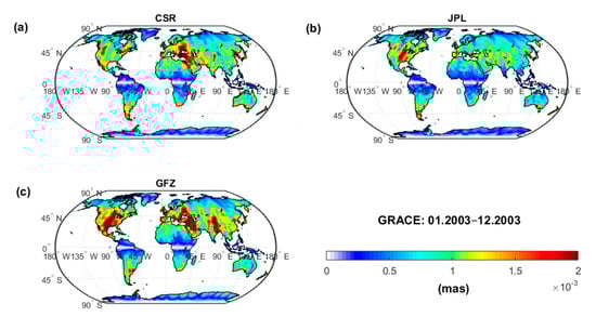
Figure 3.
Maps of RMS of differences between the mean GRACE solution (mean of data from CSR, JPL, and GFZ) and (a) HAM/CAM from CSR, (b) HAM/CAM from JPL, and (c) HAM/CAM from GFZ for 2003 (initial period of the GRACE mission).
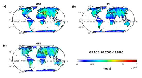
Figure 4.
Maps of RMS of differences between the mean GRACE solution (mean of data from CSR, JPL, and GFZ) and (a) HAM/CAM from CSR, (b) HAM/CAM from JPL, and (c) HAM/CAM from GFZ for 2006 (the period of best GRACE performance). The values are given in mas.
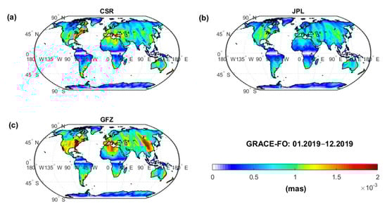
Figure 5.
Maps of RMS of differences between the mean GRACE-FO solution (mean of data from CSR, JPL, and GFZ) and (a) HAM/CAM from CSR, (b) HAM/CAM from JPL, and (c) HAM/CAM from GFZ for 2019 (initial period of the GRACE-FO mission). The values are given in mas.
3.2. External Validation of GRACE- and GRACE-FO-Based HAM/CAM Estimates
We now evaluate GRACE/GRACE-FO-based HAM/CAM estimates by comparing them with the external GAO dataset. First of all, we compare the variability of HAM/CAM and GAO series by analyzing the STD of each series (Table 2). The STD values show the higher variability of GSM-based HAM/CAM than TWS-based HAM/CAM, as reported in Section 3.1 (Figure 1). This is probably because of the non-removal of residual ocean signal in the GSM data. In general, for GRACE, TWS-based HAM/CAM underestimates the standard deviation of GAO (especially for χ2), whereas GSM-based HAM/CAM rather overestimates it (except for the CSR series). For GRACE-FO estimates, the TWS data provide higher STD consistency with GAO for χ1, whereas STD of GSM-based HAM/CAM agree better with STD of GAO for χ2. However, the fact that GAO series have visibly smaller variability for the GRACE-FO period than for the period of GRACE activity can have an impact on STD consistency between GAO and HAM/CAM.
Table 2.
Standard deviation (STD) of GAO and HAM/CAM (from GSM and TWS) series and trends in GAO and HAM/CAM (from GSM and TWS) series. Trend errors are given in brackets.
The trend values shown in Table 2 indicate that there are visible differences in trends between GSM-based and TWS-based HAM/CAM. This results from the fact that in GSM-based HAM/CAM, the GIA signal is retained, while in TWS-based HAM/CAM, GIA signatures are eliminated. It is also noticeable that trends for GRACE Level-2 data are more consistent with GAO trends in terms of their signs than trends for GRACE Level-3 data, because, similar to GSM-based HAM/CAM, GAO have trends due to GIA not being removed. Objective evaluation of HAM/CAM trends for GRACE-FO is not possible due to limited data length, however, they are reported for completeness.
Obviously, it is not possible to objectively compare results from GRACE and GRACE-FO as these two missions are over different time intervals so the signal content would not be comparable. Moreover, there are different lengths of data for the two missions: the GRACE-FO time series considered here has a length of only 19 months (June 2018 to December 2019), whereas the time series for GRACE runs for 163 months (April 2002 to June 2017 with occasional gaps). In addition, observations from the first months of the GRACE-FO may be less accurate than observations from future months, for example because there remains a need for full instrument calibration. However, we try to verify if the current level of agreement between HAM/CAM and GAO in the initial period of the GRACE-FO mission is similar to the level of agreement between HAM/CAM and GAO in the initial, best, and terminal phase of the GRACE. To do this, we select three 19-month periods that are distinguished by different accuracies of GRACE observations:
- June 2003 to December 2004 (initial period of the GRACE mission),
- June 2007 to December 2008 (best GRACE performance),
- June 2015 to December 2016 (terminal phase of the GRACE mission).
The fourth time interval considered (June 2018 to December 2019) relates to the period of GRACE-FO activity.
In order to evaluate GRACE and GRACE-FO-based HAM/CAM, for each time interval and for each equatorial component of HAM/CAM separately, we produced scatter plots showing the relationship between HAM/CAM and GAO (Figure 6, Figure 7, Figure 8, Figure 9, Figure 10, Figure 11, Figure 12 and Figure 13). The red lines in the plots were fitted to the data points using the least squares method; the closer the points to the red line, the higher the relationship between the series. To assess the quality of GRACE/GRACE-FO-based HAM/CAM in each time interval, we introduce the following parameters: correlation coefficients, RMSE, and relative explained variance. The latter indicator shows the variability agreement between the reference series (here GAO) and the evaluated series (here HAM/CAM):
where varexp is the relative explained variance, var(GAO) is the variance of the GAO series, and var(GAO−HAM/CAM) is the variance of differences between GAO and HAM/CAM. The most desirable value for this parameter is 100%. The values of all three parameters are shown on the scatter plots (Figure 6, Figure 7, Figure 8, Figure 9, Figure 10, Figure 11, Figure 12 and Figure 13).
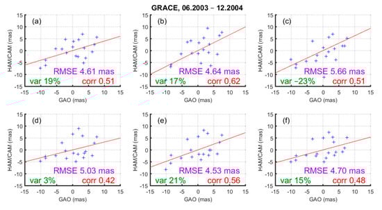
Figure 6.
Scatter plots showing the relationship between the χ1 component of GAO and HAM/CAM from (a) CSR GSM, (b) JPL GSM, (c) GFZ GSM, (d) CSR TWS, (e) JPL TWS, and (f) GFZ TWS. The red line was fitted to the data points using the least squares method. The values in purple indicate the RMSE, the values in red (corr) indicate the correlation coefficients between series, and the values in green (var) indicate the relative explained variances. The considered time period is June 2003 to December 2004. Note that the critical value of correlation coefficient for 12 independent points and a 95% confidence level is 0.50, while the standard error of the difference between two correlation coefficients is 0.47. All the parameters were computed after removal of trends.
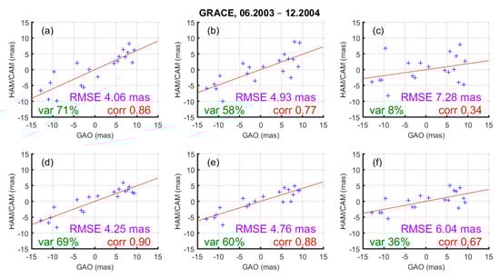
Figure 7.
Scatter plots showing the relationship between the χ2 component of GAO and HAM/CAM from (a) CSR GSM, (b) JPL GSM, (c) GFZ GSM, (d) CSR TWS, (e) JPL TWS, and (f) GFZ TWS. The red line was fitted to the data points using the least squares method. The values in purple indicate the RMSE, the values in red (corr) indicate the correlation coefficients between series, and the values in green (var) indicate the relative explained variances. The considered time period is June 2003 to December 2004. Note that the critical value of correlation coefficient for 12 independent points and a 95% confidence level is 0.50, while the standard error of the difference between two correlation coefficients is 0.47. All the parameters were computed after removal of trends.
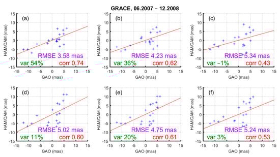
Figure 8.
Scatter plots showing the relationship between the χ1 component of GAO and HAM/CAM from (a) CSR GSM, (b) JPL GSM, (c) GFZ GSM, (d) CSR TWS, (e) JPL TWS, and (f) GFZ TWS. The red line was fitted to the data points using the least squares method. The values in purple indicate the RMSE, the values in red (corr) indicate the correlation coefficients between series, and the values in green (var) indicate the relative explained variances. The considered time period is June 2007 to December 2008. Note that the critical value of correlation coefficient for 12 independent points and a 95% confidence level is 0.50, while the standard error of the difference between two correlation coefficients is 0.47. All the parameters were computed after removal of trends.
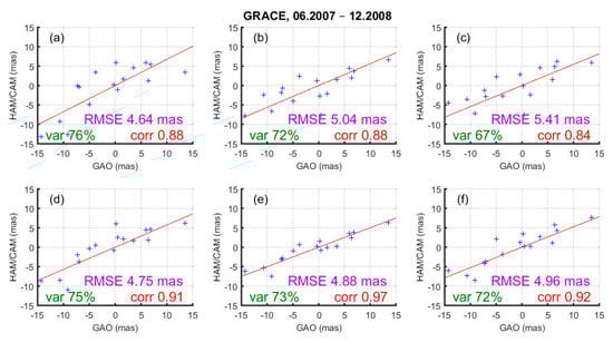
Figure 9.
Scatter plots showing the relationship between the χ2 component of GAO and HAM/CAM from (a) CSR GSM, (b) JPL GSM, (c) GFZ GSM, (d) CSR TWS, (e) JPL TWS, and (f) GFZ TWS. The red line was fitted to the data points using the least squares method. The values in purple indicate the RMSE, the values in red (corr) indicate the correlation coefficients between series, and the values in green (var) indicate the relative explained variances. The considered time period is June 2007 to December 2008. Note that the critical value of correlation coefficient for 12 independent points and a 95% confidence level is 0.50, while the standard error of the difference between two correlation coefficients is 0.47. All the parameters were computed after removal of trends.
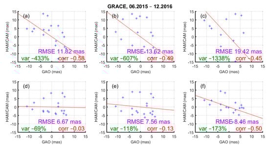
Figure 10.
Scatter plots showing the relationship between the χ1 component of GAO and HAM/CAM from (a) CSR GSM, (b) JPL GSM, (c) GFZ GSM, (d) CSR TWS, (e) JPL TWS, and (f) GFZ TWS. The red line was fitted to the data points using the least squares method. The values in purple indicate the RMSE, the values in red (corr) indicate the correlation coefficients between series, and the values in green (var) indicate the relative explained variances. The considered time period is June 2015 to December 2016. Note that the critical value of correlation coefficient for 12 independent points and a 95% confidence level is 0.50, while the standard error of the difference between two correlation coefficients is 0.47. All the parameters were computed after removal of trends.
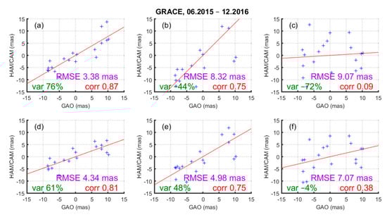
Figure 11.
Scatter plots showing the relationship between the χ2 component of GAO and HAM/CAM from (a) CSR GSM, (b) JPL GSM, (c) GFZ GSM, (d) CSR TWS, (e) JPL TWS, and (f) GFZ TWS. The red line was fitted to the data points using the least squares method. The values in purple indicate the RMSE, the values in red (corr) indicate the correlation coefficients between series, and the values in green (var) indicate the relative explained variances. The considered time period is June 2015 to December 2016. Note that the critical value of correlation coefficient for 12 independent points and a 95% confidence level is 0.50, while the standard error of the difference between two correlation coefficients is 0.47. All the parameters were computed after removal of trends.
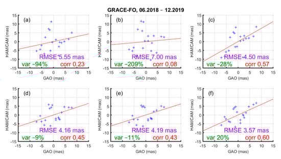
Figure 12.
Scatter plots showing the relationship between the χ1 component of GAO and HAM/CAM from (a) CSR GSM, (b) JPL GSM, (c) GFZ GSM, (d) CSR TWS, (e) JPL TWS, and (f) GFZ TWS. The red line was fitted to the data points using the least squares method. The values in purple indicate the RMSE, the values in red (corr) indicate the correlation coefficients between series, and the values in green (var) indicate the relative explained variances. The considered time period is June 2018 to December 2019. Note that the critical value of correlation coefficient for 12 independent points and a 95% confidence level is 0.50, while the standard error of the difference between two correlation coefficients is 0.47. All the parameters were computed after removal of trends.
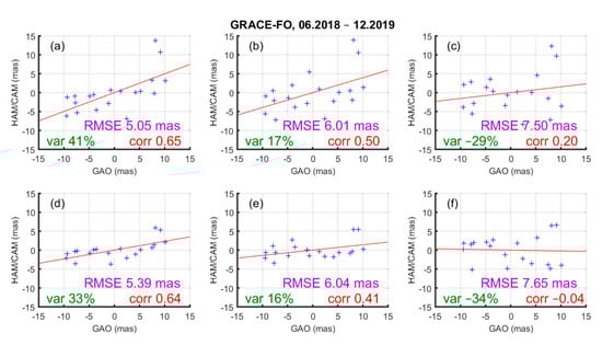
Figure 13.
Scatter plots showing the relationship between the χ2 component of GAO and HAM/CAM from (a) CSR GSM, (b) JPL GSM, (c) GFZ GSM, (d) CSR TWS, (e) JPL TWS, and (f) GFZ TWS. The red line was fitted to the data points using the least squares method. The values in purple indicate the RMSE, the values in red (corr) indicate the correlation coefficients between series, and the values in green (var) indicate the relative explained variances. The considered time period is June 2018 to December 2019. Note that the critical value of correlation coefficient for 12 independent points and a 95% confidence level is 0.50, while the standard error of the difference between two correlation coefficients is 0.47. All the parameters were computed after removal of trends.
The scatter plots for the initial period of the GRACE mission (Figure 6 and Figure 7) show that during that period, for χ1, the RMSE values range from about 4.53 to 5.66 mas, whereas for χ2 they reach values between 4.06 and 7.28 mas. The corresponding values of varexp range between −23% and 21% for χ1, and between 8% and 71% for χ2, while correlation coefficients are as high as 0.42–0.62 (χ1) and 0.34–0.90 (χ2). There is a clear difference between the results obtained for χ1 and χ2, especially in terms of the varexp and correlation values, which is mainly due to the higher sensitivity of χ2 to mass changes over continents. The Level-3 GRACE data from CSR and JPL seem to be the most appropriate for HAM/CAM determination.
Compared with the initial period of GRACE activity, the period between June 2007 and December 2008 is distinguished by the clear improvement of agreement between HAM/CAM and GAO (Figure 8 and Figure 9), which is not surprising, because the considered time interval is within the period of best GRACE performance. The results from particular processing centers are more consistent with each other compared to the previously analyzed period, as a result of the general high accuracy of GRACE measurements in 2007 and 2008. There is also no noticeable difference between results obtained using GRACE Level-2 and Level-3 data. This may indicate that the use of TWS data improves results especially during periods of reduced accuracy of GRACE measurements. However, there are still clear differences in results for χ1 and χ2, but this is rather an effect of the definition of the χ1 and χ2 equatorial components of PM excitation. The RMSE reach values of 3.58–5.34 mas for χ1 and 4.64–5.41 mas for χ2, while varexp range between −1% and 54% for χ1, and between 67% and 76% for χ2. The correlation coefficients increased to 0.43–0.74 (χ1) and 0.84–0.97 (χ2).
In the terminal phase of the GRACE activity, there is a clear increase in the errors, especially for χ1 (RMSE values vary from 6.67 to 19.42 mas) (Figure 10 and Figure 11), which is an effect of equipment deterioration and age-related battery issues. For χ2, these values range from 3.38 to 9.07 mas. In addition, varexp and correlations indicate poor consistency between HAM/CAM and GAO in χ1 as the values of these parameters are negative. Nevertheless, TWS and GSM data from CSR enable us to obtain good results for χ2 (RMSE of 3.4 and 4.3 mas for GSM and TWS, respectively; varexp of 76% and 61% for GSM and TWS, respectively; and correlations of 0.87 and 0.81 for GSM and TWS, respectively). However, these numbers are not as satisfactory as those for the period between June 2007 and December 2008.
The first results for the GRACE-FO mission were more favorable than those of the terminal phase of GRACE, but the high HAM/CAM quality that was achieved during the best GRACE period, has not yet been replicated (Figure 12 and Figure 13). Nevertheless, after full calibration of the instruments, the accuracy should increase. The current RMSE of GRACE-FO-based HAM/CAM, depending on data type and processing center, reaches 3.57–7.00 mas for χ1 and 5.05–7.65 mas for χ2, the correlation coefficients are as high as 0.08–0.60 (χ1) and −0.04–0.65 (χ2), and varexp ranges between −209% and 20% for χ1 and between −34% and 41% for χ2. Compared with data from the final years of the GRACE activity, the improvement in results for GRACE-FO is especially visible for χ1. Moreover, the discrepancy in results between χ1 and χ2 is smaller than that for GRACE.
3.3. External Validation of GSM–Based, TWS–Based and MAS-Based HAM/CAM from JPL
Finally, we compare in detail HAM/CAM estimates computed from three different GRACE/GRACE-FO data types, namely GSM, TWS, and MAS. All three datasets were processed by the JPL GRACE/GRACE-FO data center. The GFZ team has not provided their mascon solution. For the newly released mascon series from CSR (CSR RL06M v2), in contrast to data from JPL, mascons are defined on an ellipsoid. Moreover, in CSR RL06M v2, an additional correction to the ΔC30 coefficient is introduced (for GRACE-FO only). This could introduce inconsistencies while comparing with other GRACE/GRACE-FO data. Therefore, we focus here on data from JPL only.
We assess the quality of HAM/CAM estimates based on comparison with GAO. Figure 14 shows the time series of GAO, GSM-based HAM/CAM, TWS-based HAM/CAM, and MAS-based HAM/CAM. The trends for GRACE Level-2 data are most consistent with GAO trends due to not removing of GIA signals in both data types. Conversely, HAM/CAM from TWS and HAM/CAM from MAS have similar trends (see also trend values in in Table 3). Taking into consideration both the trends and STD of the series, MAS-based HAM/CAM ranks between GSM-based HAM/CAM and TWS-based HAM/CAM (Table 3).
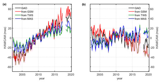
Figure 14.
Time series of (a) χ1 and (b) χ2 components of GAO and HAM/CAM computed from GRACE and GRACE-FO monthly solutions. Level-2 data (GSM) and Level-3 data (TWS and MAS) are considered. All GRACE- and GRACE-FO-based HAM/CAM series were computed using data from JPL.
Table 3.
Standard deviation (STD) of GAO and HAM/CAM (from GSM, TWS, and MAS) series and trends in GAO and HAM/CAM (from GSM, TWS, and MAS) series. All GRACE- and GRACE-FO-based HAM/CAM series were computed using data from JPL. Trend errors are given in brackets.
We now conduct a detailed evaluation of HAM/CAM computed from three different data types by presenting scatter plots together with values of RMSE, varexp, and correlation coefficients (Figure 15 and Figure 16). We consider the whole period of the GRACE activity (April 2002 to June 2017, Figure 15) and the first 19 months of GRACE-FO operation (June 2018 to December 2019, Figure 16). The plots indicate that the GRACE/GRACE-FO Level-3 data provide the lowest errors of HAM/CAM: TWS-based HAM/CAM is most consistent with GAO for χ1 (RMSE is as high as 6.06 mas for GRACE and 4.19 mas for GRACE-FO; varexp values are 39% for GRACE and −11% for GRACE-FO, correlation coefficients are 0.64 for GRACE and 0.43 for GRACE-FO), while MAS-based HAM/CAM is most consistent with GAO for χ2 (RMSE are as high as 5.66 mas for GRACE and 3.92 mas for GRACE-FO; varexp values are 62% for GRACE and 65% for GRACE-FO, correlation coefficients are 0.81 for GRACE and 0.84 for GRACE-FO). It should be remembered that χ2 is more sensitive to mass changes over land, so it can be concluded that MAS data are most appropriate to analyze water storage changes on land and assess the resulting PM excitation due to the land hydrosphere and cryosphere. Indeed, previous paper [15] showed that in studies on changes in water storage it is more appropriate to use MAS data than SH solutions. Therefore, although TWS-based HAM/CAM is in slightly a better agreement with GAO for χ1 component than MAS-based HAM/CAM, we generally recommend using MAS solution in the study of PM excitation due to land hydrosphere/cryosphere. This decision is also supported by a better STD and trend consistency between HAM/CAM and GAO for MAS data than TWS data, for both χ1 and χ2 (Table 3).
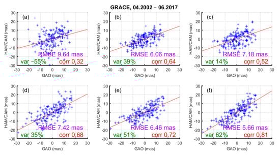
Figure 15.
Scatter plots showing the relationship between χ1 component of GAO and HAM/CAM from (a) JPL GSM, (b) JPL TWS, and (c) JPL MAS, and scatter plots showing the relationship between χ2 component of GAO and HAM/CAM from (d) JPL GSM, (e) JPL TWS, and (f) JPL MAS. The red line was fitted to the data points using the least squares method. The values in purple indicate the RMSE, the values in red (corr) indicate the correlation coefficients between series, and the values in green (var) indicate the relative explained variances. The considered time period is April 2002 to June 2017. Note that the critical value of correlation coefficient for 63 independent points and a 95% confidence level is 0.21, while the standard error of the difference between two correlation coefficients is 0.18. All the parameters were computed after removal of trends.
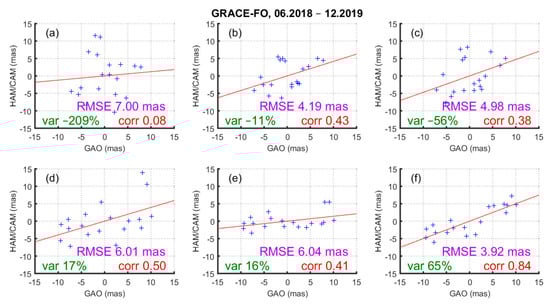
Figure 16.
Scatter plots showing the relationship between χ1 component of GAO and HAM/CAM from (a) JPL GSM, (b) JPL TWS, and (c) JPL MAS, and scatter plots showing the relationship between χ2 component of GAO and HAM/CAM from (d) JPL GSM, (e) JPL TWS, and (f) JPL MAS. The red line was fitted to the data points using the least squares method. The values in purple indicate the RMSE, the values in red (corr) indicate the correlation coefficients between series, and the values in green (var) indicate the relative explained variances. The considered time period is June 2018 to December 2019. Note that the critical value of correlation coefficient for 12 independent points and a 95% confidence level is 0.50, while the standard error of the difference between two correlation coefficients is 0.47. All the parameters were computed after removal of trends.
4. Discussion
4.1. Sources of Differences between HAM/CAM Obtained from Various GRACE and GRACE-FO Data Types
In this study, we checked the consistency between HAM/CAM computed from three GRACE/GRACE-FO data products (GSM, TWS, MAS). However, these time series are not expected to be similar because each GRACE/GRACE-FO data type was developed using different methods. First of all, we should distinguish between the two levels of GARCE and GRACE-FO data processing, namely Level-2 and Level-3. The data from Level-2 (GSM) are less processed than Level-3 data (TWS and MAS), which means that some corrections and models are not included. The first of them is ΔC20 coefficient correction. ΔC20 coefficient of geopotential is responsible for the flattening of the Earth (or Earth’s oblateness). The uncertainty of ΔC20 determined from GRACE/GRACE-FO is higher than uncertainty of ΔC20 provided from SLR measurements [62,63]. Therefore, during GRACE/GRACE-FO Level-3 data processing, ΔC20 from GRACE/GRACE-FO is replaced with a value obtained from SLR.
Another processing step in Level-3 data is adding degree-1 coefficients (ΔC10, ΔC11, ΔS11) which are responsible for geocenter position in relation to the Earth-fixed reference frame. The GRACE and GRACE-FO satellites are not able to measure these terms and the values given in GRACE/GRACE-FO Level-2 data files are equal to zero. In Level-3 data sets, these values are taken either from SLR observations or from a combination of GRACE data (from other than degree-1 coefficients) with ocean models [64]. However, it should be kept in mind that the computation of HAM/CAM from Level-2 data only requires the coefficients ΔC21 and ΔS21, so the above corrections do not affect GSM-based HAM/CAM. Similarly, the filtering of GRACE/GRACE-FO data primarily affects coefficients of higher degrees. Nevertheless, using above mentioned modifications is essential for the correct determination of HAM/CAM from TWS and MAS.
Another correction included in Level-3 data and not included in Level-2 is a GIA correction that should be applied to remove effects from postglacial rebound, but also from present ice mass changes. It is known that postglacial rebound primarily affects PM trends, but rather does not affect interannual, seasonal, and shorter HAM/CAM variations. In previous sections, we noticed that there are visible differences in trends between GSM-based HAM/CAM and TWS-based HAM/CAM (Section 3.1, Section 3.3), and between GSM-based HAM/CAM and MAS-based HAM/CAM (Section 3.3). Such trend differences mainly result from the use of GIA model in TWS and MAS data (they are both Level-3 data), which is not used in GSM (Level-2). The GIA model applied in all TWS solutions and in MAS data used in this study is the same [46], which allows for consistency between the series.
Another similarity between TWS and MAS data is that in both of them ocean signals are completely removed as a result of the masking of these areas, so only the signals from lands are preserved. In GSM series, although some atmospheric and oceanic contributions are removed using AOD data, the residual ocean impacts resulting from not removing the entire ocean signal, ocean model errors and leakage errors can affect HAM/CAM. That is why GSM-based HAM/CAM seem to be noisier and have a higher STD than TWS-based and MAS-based HAM/CAM. In GAO, similar to GSM data, the residual ocean signals are not removed (the mask is not put on ocean areas). This might be the reason why STD of GAO is more consistent with STD of GSM-based HAM/CAM. In turn, TWS-based HAM/CAM and MAS-based HAM/CAM visibly underestimate STD of GAO. Nevertheless, the overall agreement between GAO and HAM/CAM (measured with correlation coefficients, varexp and RMSE) is higher for Level-3 GRACE/GRACE-FO data than for Level-2 data. The non-removal of the total ocean mass in GSM data has an effect on especially χ1 component, which is more sensitive to mass changes over oceans, but this should not significantly affect χ2 component, which is more closely related to mass variations over lands. Although GSM-based HAM/CAM has additional ocean signals that are not present in TWS- and MAS-based HAM/CAM, both methods are reported in the literature [9,29,41,42]. Our purpose was to compare these methods even though they provide slightly different results.
Another issue is that for computation of HAM/CAM from Level-2 data, only ΔC21 and ΔS21 coefficients of geopotential are needed, while the use of TWS data requires water storage anomalies calculated from all available coefficients, the accuracy of which decreases with increasing degree and order. Therefore, the second method can lead to higher uncertainties.
4.2. Sources of Differences between HAM/CAM Obtained from GRACE and GRACE-FO Data Provided by Different Data Centers (CSR, JPL, GFZ)
This study compares HAM/CAM from GRACE and GRACE-FO data provided by three data centers (CSR, JPL, GFZ). Although the previous works showed an improvement in agreement between particular GRACE solutions for the newest realization (RL06) compared to older releases, and an increase of the consistency between HAM/CAM and GAO [8,10], the differences between particular HAM/CAM series are still non-negligible. A detailed study on this topic was performed in the work of [12]. One of the sources of the discrepancies between HAM/CAM from various data centers are different background models used to develop particular GRACE solutions, like mean gravity field model, pole tides model, ocean tides model, solid Earth tides model, AOD data, and planetary ephemerides needed for the computation of perturbations induced by celestial bodies. However, of these models, only mean gravity field model (GGM05C for CSR and JPL, EIGEN-6C4 for GFZ) and ocean tides model (FES2014 for JPL and GFZ, GOT4.8 for CSR) are different for the newest RL06 GRACE/GRACE-FO solutions. This cannot fully explain the high consistency between JPL and CSR data and the lower compatibility between GFZ and other GRACE/GRACE-FO solutions.
It should be noted that GRACE/GRACE-FO solutions provided by various institutes differ from each other not only in background models, but also in data processing methods and parametrization schemes of accelerometers, K-band ranging, and LRI measurements. They probably make a non-negligible contribution to the differences between particular GRACE/GRACE-FO solutions. However, their impact on HAM/CAM estimation is difficult to assess as not all details on the processing of GRACE/ GRACE-FO observations are available to users.
5. Conclusions
This study presented the first estimates of hydrological/cryospheric excitation of PM from the new GRACE-FO mission alongside the results obtained from the previous experiment, GRACE. In particular, the consistency among GRACE-based HAM/CAM and among GRACE-FO-based HAM/CAM computed from data provided by various institutes (CSR, JPL, and GFZ) was analyzed. External validation of HAM/CAM series was also performed by comparing with hydrological/cryospheric signals in observed excitation (GAO). The paper also showed a comparison between HAM/CAM computed from different GRACE/GRACE-FO data types, namely Level-2 data (ΔC21, ΔS21 coefficients of geopotential) and Level-3 data (TWS anomalies obtained from spherical harmonics and TWS anomalies taken from MAS data).
The conducted research demonstrated that the highest internal consistency between different GRACE and GRACE-FO HAM/CAM series can be obtained for data from JPL and CSR (correlation coefficients are above 0.80 for both GRACE and GRACE-FO; RMSE values are between 1.71 and 5.42 mas for GRACE, and between 1.00 and 3.34 mas for GRACE-FO). The earlier studies reported in [40] conducted with the GRACE RL05 solutions show similar conclusions. The HAM/CAM series computed from data provided by GFZ deviated the most from the mean and from other solutions. This problem is well known in the international scientific community and is caused probably by processing algorithm used at GFZ. We showed that the spatial distribution of HAM/CAM (shown as maps of RMSE between HAM/CAM from particular GRACE/GRACE-FO solution and HAM/CAM from mean GRACE/GRACE-FO data) was similar for all GRACE and GRACE-FO data sets, and the largest deviations from the mean spatial distribution take place in the first months of the GRACE mission (visibly larger than for GRACE-FO in its initial period). This proves that, in general, the GRACE-FO mission performs better in its initial phase than the GRACE mission in the same phase. The highest internal consistency among different GRACE/GRACE-FO-based HAM/CAM was obtained when Level-3 data are used. We also proved that HAM/CAM from particular GRACE/GRACE-FO solutions are more compatible with each other for χ2 than for χ1, which has been already reported in previous works [9,12,40,59].
The external validation of GRACE and GRACE-FO series proved that the highest consistency between HAM/CAM and GAO can be obtained when GRACE/GRACE-FO Level-3 data are used. In particular, TWS provided the highest agreement between HAM/CAM and GAO for χ1 component (for JPL, correlation coefficients were 0.64 for GRACE and 0.43 for GRCE-FO; varexp values were 39% for GRACE and −11% for GRACE-FO; RMSE values were 6.06 mas for GRACE and 4.19 mas for GRACE-FO), whereas MAS provided the highest consistency with GAO for χ2 component (for JPL, correlation coefficients were 0.81 for GRACE and 0.84 for GRACE-FO; varexp values were 62% for GRACE and 65% for GRACE-FO; RMSE values were 5.66 mas for GRACE and 3.92 mas for GRACE-FO). For the study of PM excitation due to land hydrosphere and cryosphere, we recommend using MAS data also because of the higher consistency between MAS-based HAM/CAM and GAO in terms of STD, for both equatorial components. Therefore, future research should focus on comprehensive analysis of mascons from various data centers. Currently, mascon solutions are made available by the three institutes, namely JPL, CSR, and Goddard Space Flight Center (GSFC). However, to date, only the first two processing centers provide data for both GRACE and GRACE-FO missions.
The evaluation of the first 19 months of GRACE-FO observations, which was based on comparison between HAM/CAM and GAO, demonstrated that the current level of consistency (measured with correlation coefficients, RMSE and varexp) between GRACE-FO-based HAM/CAM and GAO was similar to the consistency of GRACE-based HAM/CAM and GAO in the initial period of the GRACE mission, lower than the consistency of GRACE-based HAM/CAM and GAO in the most accurate period of GRACE, and higher than the consistency of GRACE-based HAM/CAM and GAO in the terminal phase of the GRACE. Compared with the results from GRACE, the GRACE-FO increased the agreement between HAM/CAM and GAO especially for the χ1 component. In addition, the discrepancy in results between χ1 and χ2 was reduced.
In general, the actual level of consistency between GAO and HAM/CAM from the GRACE-FO mission (correlation coefficients: 0.08 to 0.60 for χ1 and −0.04 to 0.84 for χ2; varexp: −209% to 20% for χ1 and −34% to 65% for χ2; RMSE: 3.57 to 7.00 mas for χ1 and 3.92 to 7.65 mas for χ2, depending on data type and processing center) was as expected. In the following months, after full calibration of all instruments, this accuracy is supposed to improve [65]. It should be kept in mind that, like GRACE, GRACE-FO has a design life of 5 years; however, it is believed that the activity of GRACE-FO satellites, like that of GRACE, will be much longer than this projection. This will enable scientists to continue monitoring global mass changes that affect many geophysical processes, including polar motion. As GRACE-FO progresses, its data series will increase in length, and a need to evaluate the updated HAM/CAM series will arise. This paper establishes the early indications of GRACE-based HAM/CAM and provides a framework by which the extended series can be assessed.
Author Contributions
Conceptualization, J.Ś. and M.W.; methodology, J.Ś., M.W. and J.N.; software, J.Ś.; validation, J.Ś. and M.W.; formal analysis, J.Ś.; investigation, J.Ś.; resources, J.Ś.; data curation, J.Ś.; writing—original draft preparation, J.Ś.; writing—review and editing, J.Ś., M.W. and J.N.; visualization, J.Ś.; supervision, J.Ś. and J.N.; project administration, J.Ś.; funding acquisition, J.Ś. and J.N. All authors have read and agreed to the published version of the manuscript.
Funding
This research was funded by National Science Center, Poland (NCN), grant number 2018/31/N/ST10/00209, and by the Polish National Agency for Academic Exchange (NAWA) grant number PPI/APM/2018/1/00032/U/001.
Acknowledgments
We kindly acknowledge the CSR, JPL, and GFZ teams for providing the GRACE and GRACE-FO Level-2 and Level-3 data used in this research. We would like to thank three anonymous Reviewers for their valuable comments that contributed to the improvement of the article.
Conflicts of Interest
The authors declare no conflict of interest.
References
- Barnes, R.T.H.; Hide, R.; White, A.A.; Wilson, C.A. Atmospheric angular momentum fluctuations, length-of-day changes and polar motion. Proc. R. Soc. A Math. Phys. Eng. Sci. 1983, 387, 31–73. [Google Scholar] [CrossRef]
- Lambeck, K. The Earth’s Variable Rotation: Geophysical Causes and Consequences; Cambridge University Press: Cambridge, UK, 1980. [Google Scholar]
- Greiner-Mai, H. Decade variations of the Earth’s rotation and geomagnetic core-mantle coupling. J. Geomagn. Geoelectr. 1993, 45, 1333–1345. [Google Scholar] [CrossRef]
- Adhikari, S.; Caron, L.; Steinberger, B.; Reager, J.T.; Kjeldsen, K.K.; Marzeion, B.; Larour, E.; Ivins, E.R. What drives 20th century polar motion? Earth Planet. Sci. Lett. 2018, 502, 126–132. [Google Scholar] [CrossRef]
- Youm, K.; Seo, K.W.; Jeon, T.; Na, S.H.; Chen, J.; Wilson, C.R. Ice and groundwater effects on long term polar motion (1979–2010). J. Geodyn. 2017, 106, 66–73. [Google Scholar] [CrossRef]
- Brzeziński, A.; Nastula, J.; Kołaczek, B. Seasonal excitation of polar motion estimated from recent geophysical models and observations. J. Geodyn. 2009, 48, 235–240. [Google Scholar] [CrossRef]
- Chao, B.F.; O’Connor, W.P. Global surface-water-induced seasonal variations in the Earth’s rotation and gravitational field. Geophys. J. Int. 1988, 94, 263–270. [Google Scholar] [CrossRef]
- Göttl, F.; Schmidt, M.; Seitz, F. Mass-related excitation of polar motion: An assessment of the new RL06 GRACE gravity field models. Earth Planets Space 2018, 70. [Google Scholar] [CrossRef]
- Nastula, J.; Wińska, M.; Śliwińska, J.; Salstein, D. Hydrological signals in polar motion excitation—Evidence after fifteen years of the GRACE mission. J. Geodyn. 2019, 124, 119–132. [Google Scholar] [CrossRef]
- Nastula, J.; Śliwińska, J. Prograde and retrograde terms of gravimetric polar motion excitation estimates from the GRACE monthly gravity field models. Remote Sens. 2020, 12, 138. [Google Scholar] [CrossRef]
- Śliwińska, J.; Wińska, M.; Nastula, J. Terrestrial water storage variations and their effect on polar motion. Acta Geophys. 2019, 67, 17–39. [Google Scholar] [CrossRef]
- Śliwińska, J.; Nastula, J.; Dobslaw, H.; Dill, R. Evaluating gravimetric polar motion excitation estimates from the RL06 GRACE monthly-mean gravity field models. Remote Sens. 2020, 12, 930. [Google Scholar] [CrossRef]
- Chen, J.L.; Wilson, C.R.; Zhou, Y.H. Seasonal excitation of polar motion. J. Geodyn. 2012, 62, 8–15. [Google Scholar] [CrossRef]
- Dobslaw, H.; Dill, R.; Grötzsch, A.; Brzeziński, A.; Thomas, M. Seasonal polar motion excitation from numerical models of atmosphere, ocean, and continental hydrosphere. J. Geophys. Res. 2010, 115, B10406. [Google Scholar] [CrossRef]
- Chen, J.L. Satellite gravimetry and mass transport in the earth system. Geod. Geodyn. 2018, 10, 402–415. [Google Scholar] [CrossRef]
- Brzezinski, A. Polar motion excitation by variations of the effective angular momentum function: Considerations concerning deconvolution problem. Manuscr. Geod. 1992, 17, 3–20. [Google Scholar]
- Eubanks, T.M. Variations in the orientation of the Earth. In Contributions of Space Geodesy to Geodynamics: Earth Dynamics: Geodynamic Series; Smith, D.E., Turcotte, D.L., Eds.; American Geophysical Union: Washington, DC, USA, 1993; Volume 24, pp. 1–54. [Google Scholar]
- Brzeziński, A.; Nastula, J.; Kołaczek, B.; Ponte, R.M. Oceanic excitation of polar motion from interannual to decadal periods. In International Association of Geodesy Symposia, Proceedings of the IAG General Assembly, Sapporo, Japan, 30 June–11 July 2003; Sansò, F., Ed.; Springer: New York, NY, USA, 2003; Volume 128, pp. 591–596. [Google Scholar] [CrossRef]
- Gross, R.S.; Fukumori, I.; Menemenlis, D. Atmospheric and oceanic excitation of the Earth’s wobbles during 1980–2000. J. Geophys. Res. Solid Earth 2003, 108, 2370. [Google Scholar] [CrossRef]
- Nastula, J. The regional atmospheric contributions to the polar motion and EAAM excitation functions. In Gravity, Geoid and Marine Geodesy, Proceedings of the International Symposium No. 117, Tokyo, Japan, 30 September–5 October 1996; Segawa, J., Fujimoto, H., Okubo, S., Eds.; Springer: Berlin/Heidelberg, Germany; pp. 281–288. [CrossRef]
- Nastula, J.; Ponte, R.M. Further evidence for oceanic excitation of polar motion. Geophys. J. Int. 1999, 139, 123–130. [Google Scholar] [CrossRef]
- Nastula, J.; Ponte, R.M.; Salstein, D.A. Regional signals in atmospheric and oceanic excitation of polar motion. In Polar Motion: Historical and Scientific Problems; Dick, S., McCarthy, D., Luzum, B., Eds.; Astronomical Society of the Pacific: San Francisco, CA, USA, 2000; pp. 463–472. [Google Scholar] [CrossRef]
- Nastula, J.; Ponte, R.M.; Salstein, D.A. Comparison of polar motion excitation series derived from GRACE and from analyses of geophysical fluids. Geophys. Res. Lett. 2007, 34. [Google Scholar] [CrossRef]
- Nastula, J.; Salstein, D.A.; Kołaczek, B. Patterns of atmospheric excitation functions of polar motion from high–resolution regional sectors. J. Geophys. Res. 2009, 114, B04407. [Google Scholar] [CrossRef]
- Chen, J.L.; Wilson, C.R. Hydrological excitations of polar motion, 1993–2002. Geophys. J. Int. 2005, 160, 833–839. [Google Scholar] [CrossRef]
- Chen, J.L.; Wilson, C.R.; Chao, B.F.; Shum, C.K.; Tapley, B.D. Hydrological and oceanic excitations to polar motion and length-of-day variation. Geophys. J. Int. 2000, 141, 149–156. [Google Scholar] [CrossRef]
- Hinnov, L.A.; Wilson, C.R. An estimate of the water storage contribution to the excitation of polar motion. Geophys. J. R. Astron. Soc. 1987, 88, 437–459. [Google Scholar] [CrossRef]
- Nastula, J.; Pasnicka, M.; Kolaczek, B. Comparison of the geophysical excitations of polar motion from the period 1980.0–2007.0. Acta Geophys. 2011, 59, 561–577. [Google Scholar] [CrossRef]
- Wińska, M.; Nastula, J.; Kołaczek, B. Assessment of the global and regional land hydrosphere and its impact on the balance of the geophysical excitation function of polar motion. Acta Geophys. 2016, 64, 1–23. [Google Scholar] [CrossRef]
- Wińska, M.; Nastula, J.; Salstein, D.A. Hydrological excitation of polar motion by different variables from the GLDAS model. J. Geod. 2017, 17, 7110. [Google Scholar] [CrossRef]
- Wińska, M.; Śliwińska, J. Assessing hydrological signal in polar motion from observations and geophysical models. Stud. Geophys. Geod. 2018, 63, 95–117. [Google Scholar] [CrossRef]
- Rodell, M.; Houser, P.R.; Jambor, U.; Gottschalck, J.; Mitchell, K.; Meng, C.-J.; Arsenault, K.; Cosgrove, B.; Radakovich, J.; Arsenault, K.; et al. The global land data assimilation system. Bull. Am. Meteorol. Soc. 2004, 85, 381–394. [Google Scholar] [CrossRef]
- Taylor, K.E.; Stouffer, R.J.; Meehl, G.A. An overview of CMIP5 and the experiment design. Bull. Am. Meteorol. Soc. 2012, 93, 485–498. [Google Scholar] [CrossRef]
- Güntner, A. Improvement of global hydrological models using GRACE data. Surv. Geophys. 2008, 29, 375–397. [Google Scholar] [CrossRef]
- Tapley, B.D.; Bettadpur, S.; Watkins, M.; Reigber, C. The gravity recovery and climate experiment: Mission overview and early results. Geophys. Res. Lett. 2004, 31, L09607. [Google Scholar] [CrossRef]
- Tapley, B.; Watkins, M.M.; Flechtner, F.; Reigber, C.; Bettadpur, S.; Rodell, M.; Famiglietti, J.; Landerer, F.; Chambers, D.; Reager, J.; et al. Contributions of GRACE to understanding climate change. Nat. Clim. Chang. 2019, 9, 358–369. [Google Scholar] [CrossRef] [PubMed]
- Wahr, J.; Molenaar, M.; Bryan, F. Time variability of the Earth’s gravity field: Hydrological and oceanic effects and their possible detection using GRACE. J. Geophys. Res. 1998, 103, 30205–30229. [Google Scholar] [CrossRef]
- Wouters, B.; Bonin, J.A.; Chambers, D.P.; Riva, R.E.M.; Sasgen, I.; Wahr, J. GRACE, time-varying gravity, Earths system dynamics and climate change. Rep. Prog. Phys. 2014, 77, 116801. [Google Scholar] [CrossRef] [PubMed]
- Göttl, F.; Murböck, M.; Schmidt, M.; Seitz, F. Reducing filter effects in GRACE-derived polar motion excitations. Earth Planets Space 2019, 71, 1–11. [Google Scholar] [CrossRef]
- Meyrath, T.; van Dam, T. A comparison of interannual hydrological polar motion excitation from GRACE and geodetic observations. J. Geodyn. 2016, 99, 1–9. [Google Scholar] [CrossRef]
- Seoane, L.; Nastula, J.; Bizouard, C.; Gambis, D. Hydrological excitation of polar motion derived from GRACE gravity field solutions. Int. J. Geophys. 2011. [Google Scholar] [CrossRef]
- Seoane, L.; Biancale, R.; Gambis, D. Agreement between Earth’s rotation and mass displacement as detected by GRACE. J. Geodyn. 2012, 62, 49–55. [Google Scholar] [CrossRef]
- Śliwińska, J.; Nastula, J. Determining and evaluating the hydrological signal in polar motion excitation from gravity field models obtained from kinematic orbits of LEO satellites. Remote Sens. 2019, 11, 1784. [Google Scholar] [CrossRef]
- Kornfeld, R.P.; Arnold, B.W.; Gross, M.A.; Dahya, N.T.; Klipstein, W.M. GRACE-FO: The gravity recovery and climate experiment follow-on mission. J. Spacecr. Rocket. 2019, 56, 931–951. [Google Scholar] [CrossRef]
- Gross, R. Theory of earth rotation variations. In VIII Hotine-Marussi Symposium on Mathematical Geodesy; Sneeuw, N., Novák, P., Crespi, M., Sansò, F., Eds.; Springer: Cham, Switzerland, 2015; Volume 142, pp. 41–46. [Google Scholar]
- Peltier, W.R.; Argus, D.F.; Drummond, R. Space geodesy constrains ice-age terminal deglaciation: The global ICE-6G C (VM5a) model. J. Geophys. Res. Solid Earth 2015, 120, 450–487. [Google Scholar] [CrossRef]
- Geruo, A.; Wahr, J.; Zhong, S. Computations of the viscoelastic response of a 3-D compressible Earth to surface loading: An application to Glacial Isostatic Adjustment in Antarctica and Canada. Geophys. J. Int. 2013, 192, 557–572. [Google Scholar] [CrossRef]
- Landerer, F.W.; Swenson, S.C. Accuracy of scaled GRACE terrestrial water storage estimates. Water Resour. Res. 2012, 48. [Google Scholar] [CrossRef]
- Rowlands, D.D.; Luthcke, S.B.; McCarthy, J.J.; Klosko, S.M.; Chinn, D.S.; Lemoine, F.G.; Boy, J.-P.; Sabaka, T.J. Global mass flux solutions from GRACE: A comparison of parameter estimation strategies—Mass concentrations versus Stokes coefficients. J. Geophys. Res. 2010, 115, B01403. [Google Scholar] [CrossRef]
- Luthcke, S.; Sabaka, T.; Loomis, B.; Arendt, A.; McCarthy, J.; Camp, J. Antarctica, Greenland and Gulf of Alaska land-ice evolution from an iterated GRACE global mascon solution. J. Glaciol. 2013, 59, 613–631. [Google Scholar] [CrossRef]
- Watkins, M.M.; Wiese, D.N.; Yuan, D.-N.; Boening, C.; Landerer, F.W. Improved methods for observing Earth’s time variable mass distribution with GRACE using spherical cap mascons. J. Geophys. Res. Solid Earth 2015, 120, 2648–2671. [Google Scholar] [CrossRef]
- Wiese, D.N.; Landerer, F.W.; Watkins, M.M. Quantifying and reducing leakage errors in the JPL RL05M GRACE mascon solution. Water Resour. Res. 2016, 52, 7490–7502. [Google Scholar] [CrossRef]
- Wińska, M.; Nastula, J.; Śliwińska, J.; Salstein, D. Mass and motion terms of atmospheric and oceanic angular momentum contributions to polar motion excitation. In Proceedings of the European Geosciences Union General Assembly, Vienna, Austria, 8–13 April 2018. [Google Scholar] [CrossRef]
- Bizouard, C.; Lambert, S.; Gattano, C.; Becker, O.; Richard, J.Y. The IERS EOP 14C04 solution for Earth orientation parameters consistent with ITRF 2014. J. Geod. 2018, 93, 621–633. [Google Scholar] [CrossRef]
- Jungclaus, J.H.; Fischer, N.; Haak, H.; Lohmann, K.; Marotzke, J.; Matei, D.; Mikolajewicz, U.; Notz, D.; von Storch, J.S. Characteristics of the ocean simulations in MPIOM, the ocean component of the MPI-Earth system model. J. Adv. Model. Earth Syst. 2013, 5, 422–446. [Google Scholar] [CrossRef]
- Dobslaw, H.; Wolf, I.; Dill, R.; Poropat, L.; Thomas, M.; Dahle, C.; Esselborn, S.; König, R.; Flechtner, F. A new high–resolution model of non–tidal atmosphere and ocean mass variability for de–aliasing of satellite gravity observations: AOD1B RL06. Geophys. J. Int. 2017, 211, 263–269. [Google Scholar] [CrossRef]
- Gross, R.S.; Lavallée, D.A.; Blewitt, G.; Clarke, P.J. Consistency of Earth rotation, gravity, and shape measurements. In Observing Our Changing Earth, Proceedings of the International Association of Geodesy Symposia, Perugia, Italy, 2–13 July 2007; Sideris, M.G., Ed.; Springer: Berlin/Heidelberg, Germany, 2009; Volume 133. [Google Scholar] [CrossRef]
- Sakumura, C.; Bettadpur, S.; Bruinsma, S. Ensemble prediction and intercomparison analysis of GRACE time-variable gravity field models. Geophys. Res. Lett. 2014, 41, 1389–1397. [Google Scholar] [CrossRef]
- Nastula, J.; Salstein, D.A.; Popiński, W. Hydrological excitations of polar motion from GRACE gravity field solutions. Int. Assoc. Geod. Symp. 2016, 2011, 513–519. [Google Scholar] [CrossRef]
- Encarnação, J.T.; Save, H.; Tapley, B.; Rim, H.-J. Accelerometer parameterization and the quality of gravity recovery and climate experiment solutions. J. Spacecr. Rocket. 2020, 57, 740–752. [Google Scholar] [CrossRef]
- Dahle, C.; Murböck, M.; Flechtner, F.; Dobslaw, H.; Michalak, G.; Neumayer, K.H.; Abrykosov, O.; Reinhold, A.; König, R.; Sulzbach, R.; et al. The GFZ GRACE RL06 monthly gravity field time series: Processing details and quality assessment. Remote Sens. 2019, 11, 2116. [Google Scholar] [CrossRef]
- Cheng, M.; Ries, J.C.; Tapley, B.D. Variations of the Earth’s figure axis from satellite laser ranging and GRACE. J. Geophys. Res. 2011, 116, B01409. [Google Scholar] [CrossRef]
- Cheng, M.; Tapley, B.D.; Ries, J.C. Deceleration in the Earth’s oblateness. J. Geophys. Res. Solid Earth 2013, 118, 740–747. [Google Scholar] [CrossRef]
- Swenson, S.; Chambers, D.; Wahr, J. Estimating geocenter variations from a combination of GRACE and ocean model output. J. Geophys. Res. 2008, 113, B08410. [Google Scholar] [CrossRef]
- Flechtner, F.; Landerer, F.; Save, H.; Dahle, C.; Bettadbur, S.; Watkins, M.; Webb, F. NASA and GFZ GRACE follow-on mission: Status, science, advances. In Proceedings of the EGU General Assembly 2020 (online meeting), 4–8 May 2020; pp. 4–8. [Google Scholar] [CrossRef]


Publisher’s Note: MDPI stays neutral with regard to jurisdictional claims in published maps and institutional affiliations. |
© 2020 by the authors. Licensee MDPI, Basel, Switzerland. This article is an open access article distributed under the terms and conditions of the Creative Commons Attribution (CC BY) license (http://creativecommons.org/licenses/by/4.0/).