Article

Enhanced Redundant Measurement-Based Kalman Filter for Measurement Noise Covariance Estimation in INS/GNSS Integration

1
School of Automation Science and Electrical Engineering, Beihang University, Beijing 100191, China
2
Science and Technology on Complex System Control and Intelligent Agent Cooperation Laboratory, Beijing 100074, China
*
Author to whom correspondence should be addressed.
Remote Sens. 2020, 12(21), 3500; https://doi.org/10.3390/rs12213500
Submission received: 9 September 2020 / Revised: 18 October 2020 / Accepted: 21 October 2020 / Published: 24 October 2020
(This article belongs to the Section Urban Remote Sensing)

Abstract

:
Adaptive Kalman filters (AKF) have been widely applied to the inertial navigation system (INS)/global navigation satellite system (GNSS) integrated navigation system. However, the traditional AKF methods suffer from the problems of filtering instability or covariance underestimation, especially when the GNSS measurement disturbances occur. In this paper, an enhanced redundant measurement-based AKF is developed to improve the filtering performance. The scheme is based on the mutual difference sequence derived from the redundant measurement of INS. By using the mutual difference sequence, the measurement noise covariance can be estimated without being affected by the inaccuracy estimates, hence avoiding the risk of filtering divergence. In addition, the kernel density estimation is used to estimate the GNSS measurement noise’s probability density to detect whether the Gaussian properties of the measurement noise are maintained. When the noise statistics are far from Gaussian distribution, the difference sequence will be modeled as an autoregressive process using the Burg’s method. The real variance of the difference sequence can then be updated relying on the autoregressive model in order to avoid the covariance underestimation. A field experiment was carried out to evaluate the performance of the proposed method. The test results demonstrate that the proposed method can effectively mitigate the GNSS measurement disturbances and improve the accuracy of the navigation solution.

Graphical Abstract

1. Introduction

The integrated navigation system composed of the inertial navigation system (INS) and the global navigation satellite system (GNSS) is being widely used to provide the complete navigation states (i.e., position, velocity and orientation) due to their complementary characteristics [1]. In the integrated system, INS as a self-contained system can provide high-bandwidth, low short-term noise outputs, but its output accuracy degrades over time; GNSS solutions have long-term stability in an open sky environment, but its update rate is low and the solution accuracy suffers from degradation when the ideal navigation environment changes. Therefore, the fusion of the INS and GNSS information using a Kalman filter (KF) can combine their advantages so as to prevent the drifting of INS solution and smooth the GNSS position output [2]. Furthermore, considering the different architectures for INS/GNSS integration, nonlinear filters such as extended Kalman filter (EKF), unscented Kalman filter (UKF) and particle filter (PF) are commonly used to deal with the nonlinearity of the integrated system. The method applied by the EKF algorithm for approximating these nonlinearities is the Taylor series. In the EKF method, the nonlinear function is linearized through calculating the term of the first order of the Taylor series about the state point. However, both the EKF and KF method can only obtain the optimal estimates by the criterion of minimum mean square error when the statistical properties of the system parameters are known and the measurement noises are in Gaussian distribution [3,4]. The UKF method utilizes the unscented transformation to parameterize the first two moments of the random state which undergo a nonlinear transformation. This kind of transformation does not require that the noise distribution belongs to Gaussian. Moreover, it can obtain more accurate mean and covariance than that achieved by nonlinear function approximation because of the notion that it should be easier to approximate a distribution than to linearize a nonlinear function [5]. Although the UKF algorithm seems to have considerable merit compared with the EKF method, the unknown statistical properties of noise is still a stumbling block to its optimal estimation [6]. Different from the UKF method, which is based on deterministic sampling, the PF method applies a large number of random particles to approximately represent the states’ posterior density distribution [7]. The state estimates can be then obtained from the posterior density distribution by using the Bayesian filtering theory [8]. Nonetheless, due to the large number of samples, the PF method usually requires heavy computation burden. Meanwhile, the degeneracy problem and sample impoverishment always haunt PF [9]. Therefore, the computation cost and its own flaws limit the applications of PF in real-time navigation.
In practical integration navigation applications, especially in some challenging environments such as urban canyons, foliage covered areas and open pits, the GNSS signals are subject to interference. Therefore, the measurement noise statistic characteristics are uncertain and time varying. Besides, the uncertainty involved in the system state model also has a serious influence on the process noise covariance. Considering the noise covariance variation, the conventional KF and nonlinear filters are usually unable to be directly used to estimate the navigation states. The inadequate prior assumption of the noise covariance will significantly influence the localization performance of the INS/GNSS integrated system and potentially will lead to filter divergence [10,11,12]. To improve the performance of the integrated system, the concept of adaptive Kalman filter (AKF) was employed to deal with the inadequate noise covariance [13,14]. Generally, these methods fall into four categories: Bayesian methods, maximum likelihood estimations, covariance matching approaches, and correlation techniques [15,16]. The basic idea of Bayesian methods is to obtain a recursion equation for the posterior probability density function (PDF) of the state from the measurement and then estimate the parameters by integrating the PDF. In the maximum likelihood estimation, the likelihood function is maximized to obtain the noise statistic estimates. Although both of them are theoretically sound, they require heavy computations and have been falling out of application in favor of INS/GNSS integration. Covariance matching approaches balance the trade-off between the computation and the performance. Yet the core idea behind these methods is intuitive. Thus, the matching method’s convergence is not always accurate and gives biased covariance estimates [17]. Correlation techniques are fruitful in noise covariance estimation, where a set of linear equations relating the components of the noise statistics to the autocorrelation of the innovation or residual sequences are established. Through solving these linear equations, the measurement or process noise covariance can be obtained. One of the most popular correlation methods is innovation-based adaptive estimation (IAE), in which an estimate of the noise covariance is provided by a linear transformation of the innovation covariance [18,19].
Although the IAE method can improve the accuracy of the INS/GNSS integration navigation solutions by using the estimated noise covariance, the stability of the IAE method is compromised. As well-known, the IAE method is based on the innovation, which is easily influenced by both the contaminated measurements as well as inaccurate estimates. Therefore, the estimated covariance using IAE has the risk to decline in accuracy and even results in filtering divergence, especially in the case where the statistical properties of both measurement noise and process noise are needed to be estimated [20]. Aiming for solving this problem, Zhang et al. [21] proposed a redundant measurement-based adaptive estimation (RMAE) for the INS/GNSS integrated navigation system, in which the INS solutions are used as redundant measurements to estimate the measurement noise covariances. As the estimates of the measurement noise covariance are only based on the measurements, the RMAE method is immune to the state errors. In view of this advantage, Ge et al. [22] combined the RMAE method with the algorithms for process noise covariance estimation so as to avoid the coupling problem of estimating the measurement and process noise covariance simultaneously. In the INS/GNSS navigation, however, the GNSS measurement noise may no longer be in a Gaussian distribution and the measurements are correlated in time or even involve many random outliers, especially in multipath afflicted environments. Thus, the measurement noise covariance obtained using RMAE may be underestimated due to ignoring the autocorrelation when the mutual difference sequence is non-Gaussian. To improve the position accuracy and reliability, Dhital et al. [23] assumed that the GNSS measurement noise follows a heavy-tailed distribution in the challenging environments such as deep canyons and adjusted the measurement noise covariance using a scalar based on the acceleration consistency between the GNSS and INS. Ghaleb et al. [24] modeled the correlated measurement residual sequence as a first-order autoregressive process AR(1), and then used the Yule-Walker method to estimate the measurement noise covariance. The measurement residual sequence collected in estimation, however, neglects the steady-state error of GNSS and INS. Therefore, the measurement residual sequence is not capable of representing the measurement noises properly. Moreover, the randomness testing based on the improper measurement residuals may lead to the misjudgment of the optimality of KF.
In this work, we focus on the measurement noise covariance estimation. Based on the RMAE method, an enhanced redundant measurement-based adaptive Kalman filter is developed, which extends RMAE to the case with correlated measurements. Furthermore, the abnormal observations are also considered. The random weighting method is introduced into the measurement covariance estimation to control outliers’ precision levels, which overcomes the limitation of the RMAE method; that is, all samples from historical epochs make an equivalent contribution to the measurement covariance estimation. The improved RMAE method can accurately achieve the varying measurement noise covariance without relying on states estimation. Thus, the coupling problem of covariance estimation can be solved by combining the enhanced RMAE method with other schemes for the estimation of process noise covariance.
The remainder of this paper is organized as follows: Section 2 describes the INS/GNSS tightly coupled scheme briefly; Section 3 introduces the implementation of the enhanced redundant measurement-based adaptive Kalman filter; the field test results are discussed in Section 4, and Section 5 summarizes this paper with a conclusion.

2. INS/GNSS Tightly Coupled Integration

According how GNSS measurements are used in the integration algorithm, the way of corrections applied to the inertial navigation solution, and whether the GNSS user equipment is aided, the INS/GNSS integration architecture can be mainly divided into three groups: loosely coupled, tightly coupled and ultra-tightly coupled integration systems [25].
The loosely coupled system has a simple structure, where the outputs of the GNSS navigation filter are directly input as measurements to the integration filter. However, the errors of the filtering outputs are time correlated, so the usage of a cascaded architecture may disrupt the state estimation of KF. Different from the loosely coupled integration, the GNSS navigation filter and the integration filter are combined into one in the tightly coupled integration to get rid of the statistical problem of cascading. Furthermore, this architecture has a suppression effect on GNSS multipath and still works even when the number of visible satellites drops to one [26]. The main feature of an ultra-tightly coupled system is that the INS is used to aid GNSS receiver acquisition and tracking. In the ultra-tight coupling, the corrected INS solution is used to generate the commands of the GNSS receiver’s numerically controlled oscillator. Thus, compared with tight coupling, the ultra-tightly coupled integration can operate with a lower tracking bandwidth. Nevertheless, this architecture is usually very complex and computationally intensive, and a new interface between GNSS receiver and INS need to be designed. Hence, the tightly coupled INS/GNSS integration is widely preferred for its good robustness as well as easy implementation.

2.1. Dynamic Model

In the tightly coupled integration, the system state model can be established by combining an INS and a GNSS state error propagation. The states of INS consist of the attitude error φn, velocity error δVn and position error (δL, δλ, δh), together with the gyroscope drift εb and accelerometer error b, while the states additionally considered in GNSS are the GNSS user equipment’s clock offset δtu and its drift δtru.
The attitude error propagation in the local-level frame, which can also be stated as the navigation (n-)frame, is formulated as
φ ˙ n = ( ω i e n + ω e n n ) × φ n + ( δ ω i e n + δ ω e n n ) C b n ε b
where ω i e n is the earth rate expressed in n-frame, ω e n n denotes the rate of n-frame with respect to the earth-centered, earth-fixed (e-)frame, C b n is the direction cosine matrix from the body (b-)frame to n-frame.
The transition function of the velocity error vector in the n-frame can be described as
δ V ˙ n = f n × f n + δ V n × ( 2 ω i e n + ω e n n ) + V n × ( 2 δ ω i e n + δ ω e n n ) + δ g n + C b n b
where f n and δ g n represent the specific force and gravitational error, respectively.
The position error propagation is shown as follows
{ δ L ˙ = δ V y n R M + h V y n ( R M + h ) 2 δ h δ λ ˙ = δ V x n ( R N + h ) cos L V x n ( R N + h ) 2 cos L δ h + V x n · tan L ( R N + h ) cos L δ L δ h ˙ = V z n
where δL, δλ, δh are the position error components in the latitude, longitude and height. V x n , V y n , V z n are the velocity components in the east, north, and up direction. RM and RN denote the meridian and transverse radius of curvature, respectively.
The error model of gyroscope is assumed to be the combination between zero-offset bias and first-order Gauss-Markov (GM) process, thus
{ ε = ε b + ε r ε ˙ b = 0 ε ˙ r = 1 T g ε r + ω g
where ε b and ε r denote gyroscope bias and first-order GM process, respectively. T g is the correlation time, ω g is the driving noise.
The stochastic model for accelerometer error is modeled as
˙ b = 1 T a b + w a
where T a is the correlation time and w a is Gaussian white noise.
For the state errors of GNSS, the propagation functions are
{ δ t ˙ u = δ t r u + w u δ t ˙ r u = 1 T r u δ t r u + w r u
where Tru is the correlation times, wu and wru are Gaussian white noises.
The error propagation model of the measurements can be represented as follows
{ δ ρ i = ρ G i ρ I i δ ρ ˙ i = ρ ˙ G i ρ ˙ I i
where ρ G i and ρ ˙ G i are the pseudo-range and pseudo-range rate, respectively. ρ I i and ρ ˙ I i represent the INS-driven pseudo-range and pseudo-range rate.
The pseudo-range ρ G i and pseudo-range rate ρ ˙ G i can be calculated using the broadcasted ephemeris from the satellites, whose models are as follows
{ ρ G i = r i + ( δ t u δ T i ) c + Δ i o n i + Δ t r o p i + v ρ i ρ ˙ G i = r ˙ i + ( δ t ˙ u δ T ˙ i ) c + v ρ ˙ i r i = ( x x i ) 2 + ( y y i ) 2 + ( z z i ) 2 r ˙ i = x x i r i x t + y y i r i y t + z z i r i z t
where r i denotes the true geometric distance between the receiver and satellite, and r ˙ i is the true range rate. δ T i and δ T ˙ i are the satellite clock offset and drift which can be directly obtained from the broadcasted ephemeris. c is the speed of light. Δ i o n and Δ t r o p are propagation delays of ionosphere and troposphere, respectively. These propagation errors can be mitigated by the Klobuchar model and troposphere delay models, such as Hopfield and Egnos models [27,28]. v ρ i and v ρ ˙ i are the measurement noise. (x,y,z) denotes the true position of the receiver in e-frame and (xi,yi,zi) is the position of the satellite, which can also be obtained from the ephemeris.
The INS-driven pseudo-range ρ I i and pseudo-range rate are represented as
{ ρ I i = ( x I x i ) 2 + ( y I y i ) 2 + ( z I z i ) 2 ρ ˙ I i = x I x i ρ I i x I t + y I y i ρ I i y I t + z I z i ρ I i z I t
where (xI,yI,zI) denotes the inertial measurement unit’s position in the e-frame, which can be converted from the INS position solution.

2.2. Navigation Fusion with EKF

The non-linearity of the measurement model limits the application of KF. Thus, an EKF method is used to fuse the outputs of the INS and GNSS system. In the EKF method, the non-linear models are linearized applying Taylor series expansion, which makes the measurement models suitable for the linear filtering conditions. The implementation of EKF can be described as follows
Time Updating
{ X ^ k / k 1 = F k , k 1 X ^ k 1 P k / k 1 = F k , k 1 P k 1 F k , k 1 T + Γ k 1 Q k 1 Γ k 1 T
where X ^ k 1 is the state estimate at time k−1 and X = [φn, δVn, δL, δλ, δh, εb, εr, b, δtu, δtru], Pk−1 is the estimation covariance. X ^ k / k 1 and Pk/k−1 denote the state prediction and prediction covariance. Fk,k−1 is the state transition matrix. Γ k 1 and Qk−1 are the noise-driven matrix and process noise covariance matrix, respectively.
Measurement Updating
{ X ^ k = X ^ k / k 1 + K k ( Z k H k X ^ k / k 1 ) K k = P k / k 1 H k T ( H k P k / k 1 H k T + R k ) 1 P k = ( I K k H k ) P k / k 1
where Zk denotes the difference between the GNSS pseudo-range (rate) and the INS-driven pseudo-range (rate). Hk is the measurement matrix and H k = h / X ^ k / k 1 , in which h represents the nonlinear measurement function. Kk denotes the Kalman gain and Rk is the measurement noise covariance matrix.
For the INS/GNSS tightly coupled system, the EKF method is the problem. Although it can solve the nonlinear filtering problem and obtain better navigation results, the time-varying measurement noise covariance and abnormal observations caused by the disturbances of challenging environments may result in inaccurate solutions or even divergence problems. Therefore, the measurement noise covariance used in the filter should be adapted to that of the real-time environments.

3. Enhanced Redundant Measurement-Based AKF

The RMAE method is immune to the inaccurate estimates and performs well in the case where the measurement stochastic noises are Gaussian. Nonetheless, the assumption of the white noise for GNSS measurement is not reasonable, especially in the harsh environment where the multipath errors are correlated over time. In addition, the outliers involved in the measurements will also limit the accuracy of the covariance estimation. Thus, an enhanced redundant measurement-based AKF scheme is developed in this section. The enhancement consists of three parts: a measurement-based robust adaptive noise covariance estimation for Gaussian noise, a switching strategy between the RMAE method and the Burg’s algorithm according to the statistics analysis of the second-order mutual difference sequences, and the measurement noise covariance estimation for non-Gaussian noise.

3.1. Redundant Measurement-Based Robust Adaptive Measurement Noise Covariance EstimationSubsection

The observation equations expressed in (8) and (9) show that there are two separate observations available for the same measurement values. GNSS provides the pseudo-range and pseudo-range rate directly, while INS provides them in an implicit manner. Based on the RMAE method, the measurements ZGNSS and ZINS from GNSS and INS can respectively be modeled as [29]
{ Z G N S S ( k ) = Z ( k ) + f G N S S ( k ) + V G N S S ( k ) Z I N S ( k ) = Z ( k ) + f I N S ( k ) + V I N S ( k )
where Z(k) denotes the true measurement at time epoch k, fGNSS(k) and fINS(k) are the steady-state errors of the measurements, VGNSS(k) and VINS(k) are mutually independent Gaussian noises.
Subtracting every two adjacent measurements, the difference sequences of the GNSS and INS measurement yield as
{ Δ Z G N S S ( k ) = Z G N S S ( k ) Z G N S S ( k 1 ) = Z ( k ) Z ( k 1 ) + f G N S S ( k ) f G N S S ( k 1 ) + V G N S S ( k ) V G N S S ( k 1 ) Δ Z I N S ( k ) = Z I N S ( k ) Z I N S ( k 1 ) = Z ( k ) Z ( k 1 ) + f I N S ( k ) f I N S ( k 1 ) + V I N S ( k ) V I N S ( k 1 )
Then, the second-order mutual difference sequence of the measurements can be calculated as
Z ( k ) = Δ Z G N S S ( k ) Δ Z I N S ( k ) V G N S S ( k ) V G N S S ( k 1 ) [ V I N S ( k ) V I N S ( k 1 ) ]
where the steady item f of the measurement errors is much smaller than the noise, so it can be neglected after subtraction in (14).
The two separate measurement noises are uncorrelated and zero-mean,
{ E [ V G N S S ( k ) V I N S T ( k ) ] = 0 E [ V G N S S ( k ) V G N S S T ( k 1 ) ] = 0 E [ V I N S ( k ) V I N S T ( k 1 ) ] = 0 E [ Z ( k ) ] = 0
where E[ ] is the expectation operator.
Thus, the autocorrelation of the second-order mutual difference sequences can be written as
E [ Z ( k ) Z T ( k ) ] = E [ V G N S S ( k ) V G N S S T ( k ) ] + E [ V G N S S ( k 1 ) V G N S S T ( k 1 ) ] + E [ V I N S ( k ) V I N S T ( k ) ] + E [ V I N S ( k 1 ) V I N S T ( k 1 ) ]
On the other side, the INS error accumulation is much smaller than the GNSS error in a short term. Therefore, the measurement noise covariance of GNSS can be approximated as
R G N S S = E [ V G N S S V G N S S T ] E [ Z ( k ) Z T ( k ) ] / 2
The calculation of the autocorrelation E[∇Z(k)∇ZT(k)] can utilize a limited number of samples of the second-order mutual difference sequence,
E [ Z ( k ) Z T ( k ) ] = 1 M m = 0 M 1 Z ( k m ) Z T ( k m )
where M denotes the size of the window, which is chosen by experience as it implies a trade-off between the smoothness and sharpness of the covariance estimation.
The RMAE method is decoupled from state estimation errors and suitable for the case without any random outliers involved in the GNSS measurement. However, if the abnormal observations occur, the samples from different sequences are likely to be contaminated and cannot accurately describe the statistical properties of the measurement noise, thus leading to the bias for measurement noise covariance estimation. To improve the robustness of the RMAE method, the random weights concept [30] is applied to (18), the autocorrelation can be then obtained using random weighting estimation as
E [ Z ( k ) Z T ( k ) ] = 1 M m = 0 M 1 w m Z ( k m ) Z T ( k m )
where wm denotes the random weighting factor from the Dirichlet distribution, which meets the condition m = 0 M 1 w m = 1 . The details on their determination can be found in [31].

3.2. Detection of GNSS Measurement Noise Statistics

Since the GNSS measurements are likely to be disturbed by the surroundings around the GNSS receiver, the statistical properties of the measurement noise may be far from the assumption and change to be non-Gaussian as well [32]. Before the stage of covariance estimation for the correlated noise, a detection to determine whether the measurement noise is Gaussian or not is introduced first in this subsection.
Considering the disturbance of the challenging environment would contaminate the observation’s statistical properties significantly, it is not easy to find out which family of the distribution the observation is from when the disturbance occurs. Unlike the parametric estimation assuming that the observed data belong to a given parametric family of distributions, the kernel density estimation (KDE) as a nonparametric estimation just assumes that the probability density of distribution exists [33,34]. So, the KDE method can be used to estimate the probability density under a less rigid assumption about the measurement noise statistics.
For the sake of testing accuracy, instead of innovation or residual which is also influenced by the inaccurate estimates, the second-order mutual difference sequence that relies only on the measurement is used to test the statistical properties of the measurement noise. Suppose that the independent samples ∇Z1, ∇Z2, …, ∇ZN are extracted from the second-order mutual difference sequence, the PDF of the data sequence can be estimated by KDE method as
f ^ n ( z ) = 1 N h i = 1 N K ( z Z i h )
where N is the size of sampling window, h is called bandwidth, K(⋅) denotes the kernel function.
Generally, the global estimation accuracy of f ^ n ( z ) is measured with the mean integrated square error (MISE), which is defined by
M I S E [ f ^ n ( z ) ] = E { f ^ n ( z ) f n ( z ) } 2 d z
Theories and experiments have verified that there is very little influence on the biases of MISE when the different kernel functions are selected in the context of sufficient sample size [35]. Therefore, the kernel function is commonly chosen as the Gaussian kernel function in practice, which is defined as
K ( u ) = 1 2 π e u 2 2
Along with the Gaussian kernel function, the optimal bandwidth that minimizes the MISE can be obtained by the rule of thumb [33]
h o p t = 1.06 σ N 1 / 5
where σ is the variance of the observed sequence, which can be obtained by the adaptive estimation described in Section 3.1.
According to the definition of PDF, the probability of the data falls around z can be written as
f ( z ) = d F ( z ) d z = lim h 0 F ( z + h / 2 ) F ( z h / 2 ) h
where F(z) denotes the cumulative distribution function.
Equation (24) indicates that f(z) can represent the probability of each data point that falls around z in the second-order mutual difference sequence. Furthermore, the data’s credibility can be measured through the probability as well. As illustrated in Figure 1, the dashed lines represent the individual bumps placed at the samples from the difference sequence interval { z } t 1 t n and the solid line is the density estimate which is constructed though adding each bump up. When the current datum sample zt shown by the red circle appears at the edge of the kernel density estimate, the probability of this point is very small. So, the red datum point is not likely to be from the same PDF of the previous data { z } t 1 t n and it implies that the GNSS measurement may be contaminated by the surroundings. If zt represented by the blue circle falls in the interior of the kernel density estimate, it is determined that this point belongs to the same PDF as the previous data { z } t 1 t n . The credibility of the current datum can directly be calculated by (20) in real time. If the measurement noise is normal, the credibility of each datum will satisfy the condition that f ^ n ( z t ) > K ( 3 σ ) ; Otherwise the measurement disturbance is inferred to occur and the Gaussian properties of the measurement noise may change when the condition does not hold continuously.

3.3. Measurement Noise Covariance Estimation for Non-Gaussian Noise

The RMAE method is sensitive to the correlated errors induced by the environmental noises that affect the GNSS receiver. Ignoring this autocorrelation of the measurement, especially in the multipath environment, can lead to underestimation of the measurement noise covariances. Affected by these underestimates, the filter will trust the measurement’s correctness more and cause serious implications on the filtering performance. Therefore, when the changes of the Gaussian properties of the measurement noise are detected, the second-order mutual difference sequence should be considered as a corrected sequence rather than a Gaussian noise process. Ghaleb et al. [24] used an AR(1) process to describe the corrected noise. However, the autoregressive model order also has to be estimated according to the practical noise process. Furthermore, the Yule-Walker method is unstable and may lead to poor parameter estimation in some special cases [36].
The Burg’s method is a widely employed algorithm for autoregressive modelling as it can provide reliable parameter estimates and a stable model on the contrary to the Yule-Walker and covariance method. Unlike the Yule-Walker method which can be expressed in a single set of equations, the Burg’s method operates on the difference sequence in iterations. Once the autoregressive model order p of the difference sequence is estimated using Akaike’s criterion [37], the Burg’s recursion can be implemented as follows [38,39].
Step1: Initialize the AR coefficients a 0 ( 0 ) = 1 as well as the forward prediction error vector f 0 ( 0 ) and the backward prediction error vector b 0 ( 0 ) using the difference sequence, namely,
f 0 ( 0 ) = b 0 ( 0 ) = [ Z 1 , Z 2 , , Z N ]
where N denotes the number of difference sequence samples.
Step2: Calculate the reflection coefficient
k l = 2 n = l N f n ( l 1 ) b n 1 ( l 1 ) n = l N [ ( f n ( l 1 ) ) 2 + ( b n 1 ( l 1 ) ) 2 ]
where l is the stage.
Step3: Update the prediction errors and the AR coefficients am via the Levinson-Durbin recursion.
{ f n ( l ) = f n ( l 1 ) + k l b n 1 ( l 1 ) b n ( l ) = b n 1 ( l 1 ) + k l f n 1 ( l 1 ) n = l , l + 1 , , N a m ( l ) = a m ( l 1 ) + k l a l m ( l 1 ) m = 1 , 2 , , l a l ( l ) = k l
where m and n are the symbols for counting.
Step4: Repeat steps from 2 to 3 until l = p.
After the iterations, the AR model that describes the correlation of the measurement noise can be constructed as
Z N = i = 1 p a i Z N i + v
where v is a zero-mean white noise process.
According to Ghaleb in [24], the actual variance of the difference sequence can be then obtained as follows
σ Z 2 = m = 0 M 1 Z ( k m ) Z T ( k m ) M ( 1 i = 1 p a i β i )
where βi is the autocorrelation coefficient of the difference sequence.

3.4. Implementation of the Enhanced AKF

To illustrate the above descriptions, the flowchart of the proposed enhanced redundant measurement-based AKF method is shown in Figure 2. The main steps are as follows: After the states and covariance initialization, the time-propagation is operated to predict the states using the knowledge of the a priori processing noise covariance of the INS/GNSS integrated system. Once the measurements from INS and GNSS are available, the second-order mutual difference observations will be formed. Then, the KDE-based detection approach will be applied to identify the GNSS measurement noise statistics. If the statistical properties of the measurement noise are stable and belong to the family of Gaussian distribution, the robust RMAE method will be selected. Otherwise, the measurement noise covariance will be expanded and estimated by the Burg’s method using the stream of the mutual difference observations. Finally, the updated measurement noise covariance is adopted to optimally update the state estimates during the measurement-update phase of EKF.

4. Test Results

4.1. Implementation of the Enhanced AKF

In order to validate the proposed algorithm, a field experiment was carried out in Tianjin City, China. The NovAtel IMU-ISA-100C device, whose bias offsets of the gyroscope and the accelerometer are 0.5 °/h and 1250 μg and the angle random walk of the gyroscope and the velocity random walk of the accelerometer are respectively 0.012°/ h and 100 μg/ Hz , was used to collect the raw inertial data at the rate of 100 Hz. The NovAtel GNSS receiver applied in the experiment can output the pseudo-range and pseudo-range rate data at the rate of 1 Hz. In our test, about 30 min data was collected and its post-processing positioning results processing by the NovAtel Inertial Explorer using the differential GNSS measurements in the Tightly Coupled mode were used as the ground truth. Figure 3 shows the trajectory for the test. It is clear that the GNSS outputs show a fluctuation and even deviates from the road due to the environmental disturbances when the vehicle went through the foliage or buildings.

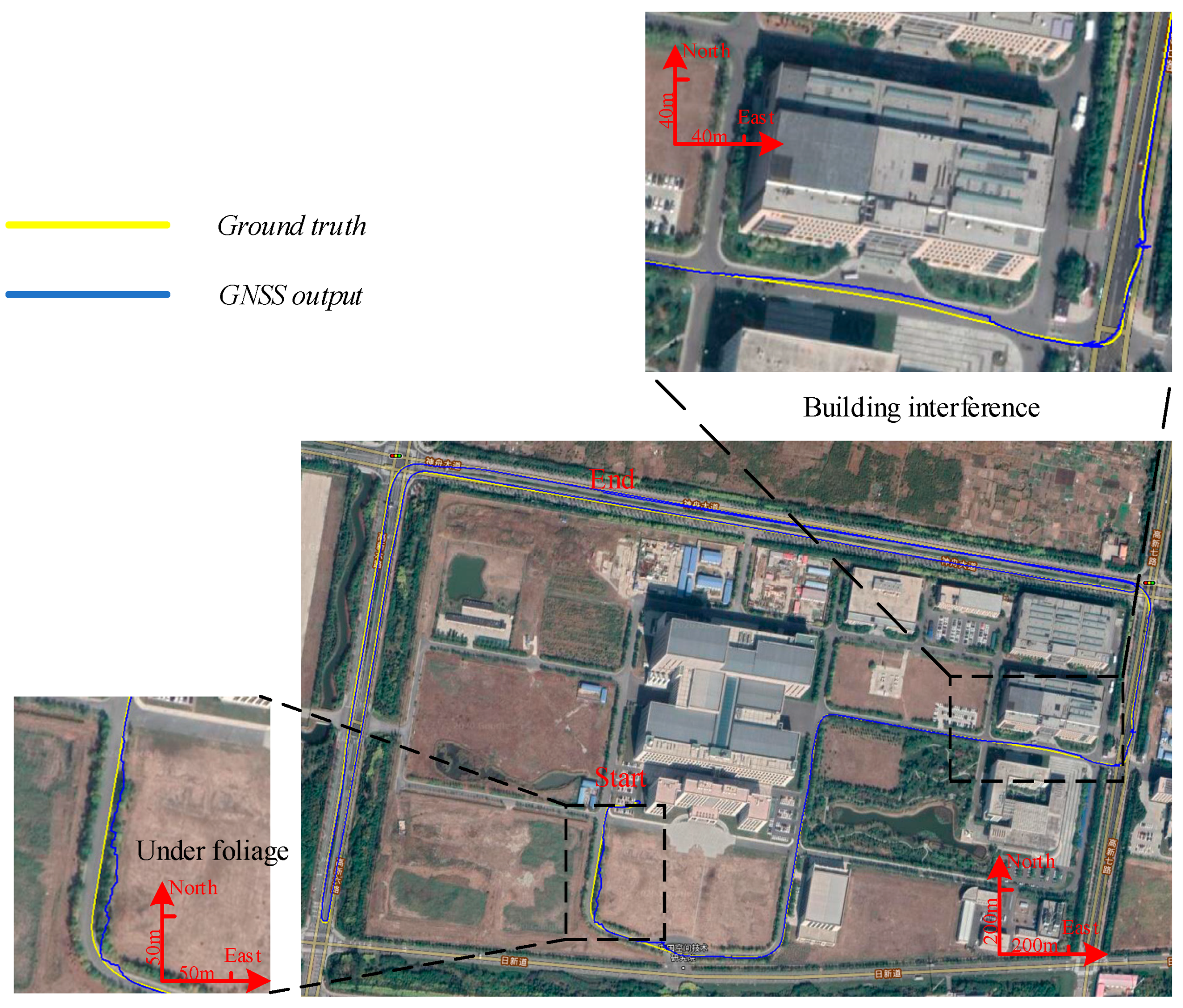
4.2. Performance Evaluation in Foliage Environment

The navigation performance of the enhanced redundant measurement-based AKF (ERMAKF) was evaluated in comparison with the standard EKF method, an enhanced innovation-based adaptive Kalman filter (EIAKF) [24], and the simple redundant measurement-based AKF (SRMAKF) which ignored the autocorrelation of the measurement disturbance. The vehicle went through the foliage during 40–120 s periods and the navigation errors with respect to the ground truth are shown in Figure 4, Figure 5 and Figure 6. Figure 7 shows the noise standard deviations of the pseudo-range ( r 1 r 4 ) and pseudo-range rate ( r 5 r 8 ) for each filter.
As shown in Figure 4, the navigation errors of the INS/GNSS tightly integrated system using the standard EKF algorithm increased significantly in the period of 50–120 s, when the vehicle was driving under the dense vegetation. The maximum error in longitude even reaches about 18 m. This can be explained by the multipath effect, which will contaminate the GNSS measurements and lead to large navigation errors. Figure 7 shows the fixed measurement noise standard deviations applied in the standard EKF. The priori values of noise covariance will lower the filtering accuracy due to the overweighed abnormal measurements. Although the EIAKF method can turn the measurement noise covariance adaptively, its noise covariance estimates may not match that of the actual measurement. This is because the estimated measurement noise covariance in the EIAKF method is based on the innovation sequence, which is also influenced by the inaccurate state estimates. In addition, the measurement residual sequence used in the EIAKF method is directly obtained by differencing the GNSS measurements and the “dead reckoning” results, which ignores the steady-state errors. It can be seen from the estimated measurement noise standard deviations of the EIAKF method in Figure 7 that the standard deviations do not update in a timely manner due to the improper difference sequence applied to the randomness testing which may lead to the misjudgment for the filtering optimality. Thus, the filtering errors of the EIAKF algorithm, as shown in Figure 4, Figure 5 and Figure 6, fluctuate quite a lot. Different from the EIAKF algorithm, the SRMAKF method estimates the measurement noise covariance relying on the redundant mutual difference sequence, which is not only immune to the state estimation error, but also considers the steady-state error of the measurement systems. Therefore, the navigation errors of the SRMAKF method are decreased compared with the EIAKF algorithm, although it causes an increase in the height error. The reason for the decrease in the height accuracy is that the altitude solutions from the GNSS are usually unsteady and even correlated in time due to the imperfect tropospheric delay model and obstructed environments. As can be seen from Figure 7, such correlation will result in the underestimation of the noise standard deviations. Compared with the EIAKF algorithm, ERMAKF takes the measurement autocorrelation into full consideration. When the measurement autocorrelation is detected using the KDE method, the Burg’s method is used to estimate the parameter of the AR model and the variance of the difference sequence is then obtained according to the AR coefficients. Figure 8, Figure 9 and Figure 10 give insight about the navigation accuracy of each algorithm in terms of the root mean square error (RMSE), which is defined as
RMSE = 1 N k = 1 N ( X ^ k X k ) 2
where X ^ k and X k are the filtering and reference states at time k, respectively.
As shown in Figure 8, the longitude solution accuracy is improved by 26.3% and 46.9% when the SRMAKF scheme is used, in comparison with the Standard EKF and EIAKF solution, respectively. It is clear that the ERMAKF scheme achieves the best performance in the longitude component, whose accuracy is further improved by 36.0% compared to the SRMAKF scheme due to the reduction in the negative influence of the measurement correlation on the noise covariance estimation. As explained before, the positioning RMSE of the EIAKF method has an increase because of the unreliable difference sequence applied in the measurement noise covariance estimation. Although the SRMAKF method can improve the longitude accuracy, the height solution deteriorates when the GNSS altitude is strongly correlated. In comparison, the height solution applying the ERMAKF scheme outperforms that of the Standard EKF and EIAKF method by 56.0% and 50.0%, respectively. The improvement in the latitude accuracy is not that significant, but it still maintains an acceptable accuracy.
The RMSE of the velocity accuracy is presented in Figure 9. It can be seen that compared with the Standard EKF solutions, the SRMAKF method improves the velocity solutions by 62.8%, 26.7% and 43.5% in the east, north and up direction, respectively. Similarly, SRMAKF obtains improvements of 68.0%, 52.2% and 18.7% compared to the EIAKF method. Moreover, the velocity accuracy can be further improved when the ERMAKF scheme is used. It should be noted that although the altitude solved by SRMAKF includes more errors, the velocity accuracy it obtains in the up direction is not the same and shows better accuracy. This is because the noise covariance of the pseudo-range and pseudo-range rate are estimated separately and these estimates will determine the measurement’s weights in filtering. Even though the accuracy of the pseudo-range and pseudo-range rates is interlinked with each other at the output from the receiver’s ranging processor, the following navigation processing will break this direct correspondence of accuracy between the two observations due to the changes in the estimated covariance while filtering. It is not surprising that the ERMAKF scheme performs better than the SRMAKF method. This is due to the fact that the SRMAKF method is not able to deal with the measurement correlations and it may underestimate the noise covariance.
As can be seen from Figure 10, although the high-precision attitude is achievable through the standard EKF method, the ERMAKF method can reduce the RMSE further, especially for the pitch and roll component. The disturbances of the abnormal GNSS measurements are rejected through de-weighting the observations, and thus the ERMAKF solutions are improved by 47.4% for the pitch component and 21.4% for the roll component compared to the standard EKF method. The discussions of the EIAKF and SRMAKF algorithms are similar as aforementioned. In general, the attitude performance using the ERMAKF scheme is satisfactory.

4.3. Performance Evaluation in Obstructed Areas

Dense buildings constitute a harsh environment, where the GNSS signals are susceptible to the disturbances. As shown in Figure 3, the positioning quality of GNSS was degraded when the vehicle passed that buildings during 260–320 s periods. In this dense building environment, the ERMAKF method can also be applied to mitigate the GNSS measurement errors. To quantify the filtering errors concisely, the RMSE in 3-D space is listed in Table 1.
Table 1 illustrates the filtering performance for different methods. It shows that although the adaptive strategies are used in the INS/GNSS integrated system, the navigation accuracy may not be improved in some special scenarios without considering the model’s influence and noise’s correlation. The EIAKF method can estimate the time-varying measurement noise covariance applying the innovation, but the mismatched error models also have a negative influence on the estimation, hence leading to the decrease in filtering accuracy. The SRMAKF method is immune to the state errors. However, the correlation between the measurements will cause the underestimation of the measurement covariance. Thus, the filtering accuracy of the SRMAKF method can still be improved. The ERMAKF method is an enhanced version of SRMAKF, in which the measurement’s autocorrelation is considered and the Burg’s method is employed to model this autocorrelation. Through classifying the measurement noise and updating their statistics, the positioning error decreases from 6.12 m to 4.60 m while applying the ERMAKF method. The velocity errors are respectively reduced by 41.4% and 55.3% compared to EIAKF and SRMAKF when the ERMAKF method is used. Meanwhile, the attitude errors obtained by EIAKF also appeared to decline, falling by 25.0% compared to the SRMAKF method. The results demonstrate that the proposed enhanced method can provide more consistent navigation solutions than the other state-of-the-art algorithms.

5. Conclusions

This paper presents a scheme of the mitigation of GNSS measurement disturbances, and the methods of RMAE and Burg’s are used to estimate the time-varying measurement noise covariance based on the statistic property of the mutual difference sequence. The scheme mainly includes the following steps: first, to obtain the mutual difference observations by using two separate measurements from INS and GNSS; second, to detect via the KDE method, whether the measurement noise statistics belong to a Gaussian distribution, and then determine the autoregressive model applying the Burg’s recursion when the Gaussian properties of the difference sequence noise are not maintained; finally, to obtain the navigation results through fusing the sensors data with the timely updating measurement noise covariance.
In the field experiment, the fusing results demonstrate that the proposed enhanced redundant measurement-based AKF method outperforms the compared methods in general. The positioning accuracy is improved by 66.0%, 20.7% and 50.0%, respectively, for longitude, latitude, and height components compared to the conventional innovation-based adaptive Kalman filter in foliage environment. However, there is a slight decrease in the yaw accuracy due to the windowing estimation errors. In addition, the ERMAKF method also obtains an improvement for the 3-dimensional navigation accuracy in the harsh environment such as dense buildings.
The current research mainly focuses on the feasibility of the proposed enhanced method and only the time-varying measurement noise covariance is inspected. In the future, the processing noise covariance estimation will be considered for improving the navigation precision, especially for the low-cost integrated system.

Author Contributions

Conceptualization, H.Z. and B.G.; methodology, B.G.; software, B.G.; validation, B.G., H.Z. and W.F.; formal analysis, B.G. and H.Z.; investigation, H.Z. and B.G.; resources, H.Z. and W.F.; data curation, H.Z.; writing—original draft preparation, B.G.; writing—review and editing, H.Z., B.G., and J.Y.; visualization, J.Y.; supervision, H.Z.; project administration, H.Z.; funding acquisition, H.Z. All authors have read and agreed to the published version of the manuscript.

Funding

This research was funded by the National Key Research and Development Program of China under Grant Nos. 2017YFC0821102 and 2016YFB0502004, and the Academic Excellence Foundation of BUAA for PhD Students.

Acknowledgments

We would like to thank the reviewers for the insightful comments and suggestions that significantly help to improve the quality of the paper. B.G. would also like to thank Huan Che and Fu Li for their inspiring talks.

Conflicts of Interest

The authors declare no conflict of interest.

References

  1. Schmidt, G.T. Navigation sensors and systems in GNSS degraded and denied environments. Chin. J. Aeronaut. 2015, 28, 1–10. [Google Scholar] [CrossRef] [Green Version]
  2. Groves, P.D. Principles of GNSS, Inertial, and Multisensor Integrated Navigation Systems; Artech House: London, UK, 2008; pp. 363–387. [Google Scholar]
  3. Kalman, R.E. A new approach to linear filtering and prediction problem. J. Basic Eng. 1960, 82, 95–108. [Google Scholar] [CrossRef] [Green Version]
  4. Jazwinski, A.H. Stochastic Processes and Filtering Theory; Academic Press: London, UK, 1970; pp. 272–279. [Google Scholar]
  5. Julier, S.J.; Uhlmann, J.K. New Extension of the Kalman Filter to Nonlinear Systems. In Proceedings of the SPIE—The International Society for Optical Engineering, Orlando, FL, USA, 21–25 April 1997. [Google Scholar]
  6. Zhe, J.; Qi, S.; He, Y.; Han, J. A novel adaptive unscented Kalman filter for nonlinear estimation. In Proceedings of the 46th IEEE Conference on Decision and Control, New Orleans, LA, USA, 12–14 December 2007. [Google Scholar]
  7. Wang, X.; Pan, Q.; Huang, H.; Gao, A. Overview of deterministic sampling filtering algorithms for nonlinear system. Control Decis. 2012, 27, 801–812. [Google Scholar]
  8. Deng, X.; Xie, J.; Ni, H. Improved Particle Filter for Target Tracking. Chin. J. Aeronaut. 2005, 18, 166–170. [Google Scholar] [CrossRef] [Green Version]
  9. Arulampalam, M.S.; Maskell, S.; Gordon, N.J.; Clapp, T. A tutorial on particle filters for online nonlinear/non-Gaussian Bayesian tracking. IEEE Trans. Signal Process 2002, 50, 174–188. [Google Scholar] [CrossRef] [Green Version]
  10. Singh, Y.; Mehra, R. Relative study of measurement noise covariance R and process noise covariance Q of the Kalman filter in estimation. IOSR J. Electr. Electron. Eng. 2015, 10, 112–116. [Google Scholar]
  11. Han, H.; Jian, W.; Du, M. GPS/BDS/INS tightly coupled integration accuracy improvement using an improved adaptive interacting multiple model with classified measurement update. Chin. J. Aeronaut. 2018, 31, 556–566. [Google Scholar] [CrossRef]
  12. Mehra, R. On the identification of variances and adaptive Kalman filtering. IEEE Trans. Autom. Control 1970, 15, 175–184. [Google Scholar] [CrossRef]
  13. Sage, A.P.; Husa, G.W. Adaptive filtering with unknown prior statistics. IEEE Trans. Autom. Control. 1970, 11, 760–769. [Google Scholar]
  14. Huang, Y.; Zhang, Y.; Wu, Z.; Li, N.; Chambers, J. A Novel Adaptive Kalman Filter with Inaccurate Process and Measurement Noise Covariance Matrices. IEEE Trans. Autom. Control 2018, 63, 594–601. [Google Scholar] [CrossRef] [Green Version]
  15. Mehra, R.K. Approaches to adaptive filtering. In Proceedings of the IEEE Symposium on Adaptive Processes (9th) Decision and Control, Austin, TX, USA, 7–9 December 1970. [Google Scholar]
  16. Meng, Y.; Gao, S.; Zhong, Y.; Hu, G.; Subic, A. Covariance matching based adaptive unscented Kalman filter for direct filtering in INS/GNSS integration. Acta Astronaut. 2016, 120, 171–181. [Google Scholar] [CrossRef]
  17. Li, X.R.; Bar-Shalom, Y. A recursive multiple model approach to noise identification. IEEE Trans. Aerosp. Electron. Syst. 1994, 30, 671–684. [Google Scholar] [CrossRef]
  18. Fang, J.; Sheng, Y. Study on innovation adaptive EKF for in-flight alignment of airborne POS. IEEE Trans. Instrum. Meas. 2011, 60, 1378–1388. [Google Scholar]
  19. Yang, Y.; Xu, T. An Adaptive Kalman Filter Based on Sage Windowing Weights and Variance Components. J. Navig. 2003, 56, 231–240. [Google Scholar] [CrossRef]
  20. Zhang, C. Approach to adaptive filtering algorithm. Acta Aeronaut. Astronaut. Sci. 1998, 19, 97–100. [Google Scholar]
  21. Zhang, H.; Chang, Y.H.; Che, H. Measurement-based adaptive Kalman filtering algorithm for GPS/INS integrated navigation system. J. Chin. Inertial Technol. 2010, 18, 696–701. [Google Scholar]
  22. Ge, B.; Zhang, H.; Jiang, L.; Li, Z.; Butt, M.M. Adaptive Unscented Kalman Filter for Target Tracking with Unknown Time-Varying Noise Covariance. Sensors 2019, 19, 1371. [Google Scholar] [CrossRef] [Green Version]
  23. Dhital, A.; Bancroft, J.; Lachapelle, G. A new approach for improving reliability of personal navigation devices under harsh GNSS signal conditions. Sensors 2013, 13, 15221–15241. [Google Scholar] [CrossRef] [Green Version]
  24. Ghaleb, F.; Zainal, A.; Rassam, M.; Abraham, A. Improved vehicle positioning algorithm using enhanced innovation-based adaptive Kalman filter. Pervasive Mob. Comput. 2017, 40, 139–155. [Google Scholar] [CrossRef]
  25. Srinivas, P.; Kumar, A. Overview of architecture for GPS-INS integration. In Proceedings of the 2017 Recent Developments in Control, Automation & Power Engineering, Noida, India, 26–27 October 2017. [Google Scholar]
  26. Zhu, Z.; Li, C. Study on real-time identification of GNSS multipath errors and its application. Aerosp. Sci. Technol. 2016, 52, 215–223. [Google Scholar] [CrossRef]
  27. Zhao, J.X.; Chang, Q.; Zhang, Q.S.; Zhang, J. Research of Ionospheric Time-Delay Error Simulation in High Dynamic GPS Signal Simulator. Chin. J. Aeronaut. 2003, 16, 169–176. [Google Scholar] [CrossRef] [Green Version]
  28. Yang, H.J.; Feng, K.M.; Xie, S.X.; Zhou, Y.Q.; Li, C. Improved GPT2w model based on BP neural network and its global precision analysis. Syst. Eng. Electron. 2019, 41, 500–508. [Google Scholar]
  29. Zhou, Q.; Zhang, H.; Li, Y.; Li, Z. An Adaptive Low-Cost GNSS/MEMS-IMU Tightly-Coupled Integration System with Aiding Measurement in a GNSS Signal-Challenged Environment. Sensors 2015, 15, 23953–23982. [Google Scholar] [CrossRef] [PubMed] [Green Version]
  30. Gao, S.; Wei, W.; Zhong, Y.; Subic, A. Sage windowing and random weighting adaptive filtering method for kinematic model error. IEEE Trans. Aerosp. Electron. Syst. 2015, 51, 1488–1500. [Google Scholar] [CrossRef]
  31. Zheng, Z. Random weighting method. Acta Math. Appl. Sin. 1987, 10, 247–253. [Google Scholar]
  32. Benzerrouk, H.; Nebylov, A. Robust nonlinear filtering applied to integrated navigation system INS/GNSS under non Gaussian measurement noise effect. In Proceedings of the 2012 IEEE Aerospace Conference, Big Sky, MT, USA, 3–10 March 2012. [Google Scholar]
  33. Silverman, B.W. Density Estimation for Statistics and Data Analysis; Chapman and Hall: London, UK, 1986; pp. 35–42. [Google Scholar]
  34. Rosenblatt, M. Remarks on some nonparametric estimates of a density function. Ann. Math. Stat. 1956, 27, 832–837. [Google Scholar] [CrossRef]
  35. Xu, Y.; Xu, N.; Feng, X. A new outlier detection algorithm based on kernel density estimation for ITS. In Proceedings of the 2016 IEEE International Conference on Internet of Things, Chengdu, China, 15–18 December 2016; pp. 258–262. [Google Scholar]
  36. Hoon de, M.J.L.; Hagen Van der, T.; Schoonewelle, H.; Dam van, H. Why Yule-Walker should not be used for autoregressive modelling. Ann. Nucl. Energy 1996, 23, 1219–1228. [Google Scholar] [CrossRef]
  37. Priestley, M.B. Spectral Analysis and Time Series; Academic Press: New York, NY, USA, 1981; pp. 372–374. [Google Scholar]
  38. Roth, K.; Kauppinen, I.; Esquef, P.A.A.; Vesa, V. Frequency warped Burg’s method for AR-modeling. In Proceedings of the IEEE Workshop on Applicat ions of Signal Processing to Audio and Acoustics, New Paltz, NY, USA, 19–22 October 2003. [Google Scholar]
  39. A Fast Implementation of Burg’s Method. Available online: https://opus-codec.org/docs/vos_fastburg.pdf (accessed on 9 September 2020).
Figure 1. Kernel density estimates showing individual Gaussian kernels and credibility detection.
Remotesensing 12 03500 g001
Figure 2. Diagram of the proposed enhanced redundant measurement-based adaptive Kalman filter (AKF).
Remotesensing 12 03500 g002
Figure 3. Ground trajectory of the field experiment.
Remotesensing 12 03500 g003
Figure 4. Position errors comparison.
Remotesensing 12 03500 g004
Figure 5. Velocity errors comparison.
Remotesensing 12 03500 g005
Figure 6. Attitude errors comparison.
Remotesensing 12 03500 g006
Figure 7. Estimated measurement noise standard deviations. (a) Estimated noise standard deviations of the pseudo-range. (b) Estimated noise standard deviations of the pseudo-range rate.
Remotesensing 12 03500 g007
Figure 8. Comparison of position root mean square error (RMSE) for different algorithms.
Remotesensing 12 03500 g008
Figure 9. Comparison of velocity RMSE for different algorithms.
Remotesensing 12 03500 g009
Figure 10. Comparison of attitude RMSE for different algorithms.
Remotesensing 12 03500 g010
Table 1. 3-Dimensional Navigation Errors for Different Methods.
AlgorithmPosition Error (m)Velocity Error (m/s)Attitude Error (°)
Standard EKF5.520.380.22
EIAKF6.240.290.25
SRMAKF6.120.380.24
ERMAKF4.600.170.18
Publisher’s Note: MDPI stays neutral with regard to jurisdictional claims in published maps and institutional affiliations.

