Abstract
Irrigation is a useful crop enhancement procedure up to the point where free surface water appears. However, over-irrigation can lead to an accumulation of free water on the soil surface, which in turn results in overland flow and a high risk of contaminant loss. The current work addresses the problem of measuring free water on the surface of agricultural soils by a real-time acoustic remote sensing method. Directional acoustic transmitter and receiver arrays are used to define a “footprint” on the ground from which changes in reflectance are sensed. These arrays are mounted on a moving irrigator. Chirp signals are used to provide along-path resolution and to ensure robustness against unwanted acoustic background noise from farm machinery and the irrigator. Field measurements have been conducted above a well-defined “quadrat” with controlled and measured water content and also with the instrument mounted on an operational irrigator. A structured light camera mounted above the footprint is used to validate surface water fraction. It is found that the areal fraction of free water on the soil surface can be reliably estimated from changes in the amplitude of the reflected sound waves. The mechanism giving rise to the observed acoustic reflectivity changes is discussed and a model is developed which agrees with normalized intensity observations with a coefficient of determination R2 between 0.65 and 0.83. The rms error between model predictions and observations is comparable to the rms variation of the measurements, indicating that there is insignificant error due to the choice of model.
1. Introduction
Precision agriculture aims to address increasing pressure on agriculture due to economic, land area, production target, and environmental challenges [1]. The focus is on improved management decisions based on digital data relating to the agricultural site and, in the case of irrigation, this means monitoring of the rate of application of water and/or the outcomes. A byproduct of increased irrigation arises when irrigation mobilizes pollutants and transports them to water bodies. Mobilization of pollutants particularly happens when the irrigation rate is greater than the rate at which the soil can accept water [2]. This critical irrigation rate can change rapidly in time and space [3,4] so good irrigation design can only partially address this issue. Currently, there are no useful sensors to provide real-time measurements of the soil surface conditions, so farmers cannot respond to the rapidly changing conditions by actively managing their irrigation. Existing sensors for irrigation management operate on either the plant or the soil. While these sensors also assist with good irrigation management, their mode of action is after a problem has occurred or they face significant physical barriers to use (e.g., requiring installation in the soil).
The soil surface typically has numerous depressions of various sizes [5,6] but will begin to smooth out as the small pockets of free water that develop normally during an irrigation event fill in some of the hollows in the surface. Free water is not bound to the soil surfaces but is instead free to flow directly into water bodies. When the pockets coalesce to form connected flow pathways [7,8,9] the free water can begin to move from the point of application. This is when water efficiency is lost and environmental harm caused. A technology that can detect free water on the soil surface during an irrigation event and control the irrigation application rate in real-time to prevent the formation of connected flow pathways would be transformative for the environment.
A number of studies have focused on the characterization of the speed and absorption of sound in different types of soils [10,11] and a few attempts to characterize sound propagation through the soil with different moisture contents [12,13], but these are in-situ rather than nonintrusive remote sensing or proximal sensing methodologies. One potential method of sensing the nature of the soil surface is to use acoustic reflection. There is a substantial literature on soil reflectivity relating to outdoor sound propagation [14], although sound propagation studies are concerned with grazing incidence and large distances not relevant to close proximity sensing from above.
The measurable quantity is the reflection coefficient or reflectivity, which is the ratio of the reflected sound intensity and the incident sound intensity. Reflectivity depends on the angle of incidence and on a quantity called the complex ground impedance. Soil is a porous material comprised of a combination of clay, silt, and sand particles, which are classified by differing average grain diameter [15]. The acoustic reflection properties of soil depend on its porosity, flow resistivity, tortuosity, steady-flow shape factor, and dynamic shape factor [12]. Porosity and flow resistivity are considered the most important soil characteristics that affect acoustic impedance. At sound frequencies f below 1 kHz, the flow resistivity has the largest effect on impedance, and above 1 kHz the porosity has the greater effect on impedance [16]. The acoustic flow resistivity is a measure of the air space volume in the soil near the surface with sound propagation being limited to around 10 mm [17].
The near-surface nature of the acoustic interaction is ideal for the purposes of sensing the presence of free water on the soil surface. The higher flow resistivity and lack of porosity of water means that it has a higher acoustic impedance than soil. The acoustic impedance is expected to have a clear increasing trend with a greater moisture content, which will plateau for saturated soil [10], [18,19]. A laboratory study [12,13] indicated that reflectance measurements can potentially give estimates of volumetric water content to ±2%. A field measurement [19], where the moisture content was measured and varied, used an acoustic impulse, with the amplitude of reflected sound doubling when the moisture content of grassland was changed from 10% to 35%. The variation in reflectance was found to vary substantially with position once the soil was wetted. There also appeared to be strong sensitivity to the air volume. The studies described above suggest that acoustic reflectance could be a useful tool for remotely sensing free water. Our goal in this study, therefore, was to develop a relatively simple and accessible technology for real-time sensing of soil surface condition, without requiring contact with the surface. Below we present the theoretical basis, design, and testing of this sensor.
2. Methods and Instrument Design
The design of a suitable proximal acoustic sensing system was guided by initial model predictions and by proof-of-concept laboratory measurements. Section 2.1 describes the sound frequency selection procedure and hardware design for the acoustic sensor. Section 2.2 deals with the sensor footprint on the ground. Finally, the temporal resolutions and electrical design of the sensor are described in Section 2.3.
2.1. Frequency Selection and Hardware Design
In order to select an appropriate sound frequency range for the purpose of this study, reflectivity from a virtual soil surface was estimated by a model for the acoustic impedance of a ground surface [14] for sound frequency ranging from 1 to 4 kHz. In doing so, the following model parameter values were selected: soil porosity = 0.3, tortuosity = 1.35, flow resistivity = 100 to 103 kPa s m−2, and pore shape factor ratio = 0.75. Simulation results are shown in Figure 1 for the frequency range 1 to 4 kHz and for an angle of incidence of 45°. The reflectivity has been normalized to that from soil of porosity 0.5 and flow resistivity 100 kPa s m−2.
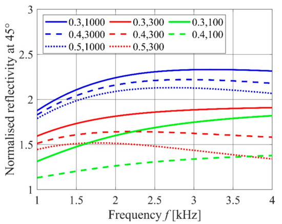
Figure 1.
Reflectivity from soil at 45° incidence normalized to the reflectivity when porosity = 0.5 and flow resistivity = 100 kPa s m−2. Porosity and flow resistivity (in kPa s m−2) are given in the legend.
From Figure 1, the greatest fractional variation is predicted to occur at the higher frequencies. Therefore, an acoustic frequency of 2.5 to 4.5 kHz was chosen for the design. An array of six speakers, with their center-to-center distance 85 mm, were used to generate short pulses of duration 2 ms directed downward at an angle of 45°. This pulse duration was selected based on doing initial measurements in the laboratory and beneath an irrigator using the speakers and microphones mounted on a test rig of height 1 m above the ground and with the horizontal separation between array centers being 2 m (see Section 3.1 below). For this geometry, and for angles of incidence and reflection at the ground being 45°, the time difference between direct (horizontal) reception and slantwise reflected reception is 2.4 ms for a sound speed of 340 m s−1. The pulses comprised sinusoidal waves of 4 cycles at 2 kHz and 8 cycles at 4 kHz. This frequency range ensures a response due to porosity, without undue absorption from the air, soil, or any overlaying pasture. The Motorola KSN1005A super horn piezo tweeters were chosen, producing sound pressure levels of 74 dB at 2 kHz and 94 dB at 4 kHz, at 1 m distance when driven with 2.8 Vrms. The speakers have dimensions of d = 85 mm.
Signal generation and data acquisition were handled with a Data Translation DT9836 unit with 16-bit synchronous input and output controlled from a laptop. The DAC drives the six speakers in parallel via a Dayton_Audio_DTA3116HP 30 W amplifier, and the ADC samples the six “microphones” in parallel. Power derives from a battery, which can be maintained via a solar panel. Data is sampled at the standard audio rate of 44,100 samples per second.
The diffraction formula for the intensity from a linear array of M speakers spaced at separations d is
I = I0(θ){sin(Mx)/[Msin(x)]}2
where x = kdsin(θ)/2 for beam angle θ and k is the wavenumber [20]. The squared term has a half-power half-width of approximately Mx = 21/2. The angular behavior of an individual speaker is described by I0(θ) which for these speakers and frequencies is approximately proportional to cos4(θ). Based on (A1) the array gave a directional beam of half-power angular width of 6° at 2.5 kHz and 4° at 4 kHz which agrees closely with the measured response, as shown in Figure 2.
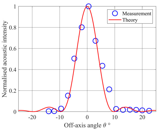
Figure 2.
Measured beam pattern at 3.4 kHz compared with theoretical expectations.
The “far field” region (Fresnel parameter > 1) for this antenna is beyond a range of about 1 m at a frequency of 4 kHz, so the beam has a range-independent far-field shape at the ground.
The KSN1005A piezoelectric speakers are also used as the 6 elements in the microphone array since a voltage is developed across a piezo crystal in response to the pressure fluctuations from an acoustic wave. The angular response when used as a microphone is the same as when used as a speaker.
2.2. Sensing Geometry and Footprint
The goal is to design an instrument to mount on a large mobile irrigator of the type shown in Figure 3. This means a design height from the ground, h, of the acoustic transmitter and acoustic receiver units should be around 2 m.
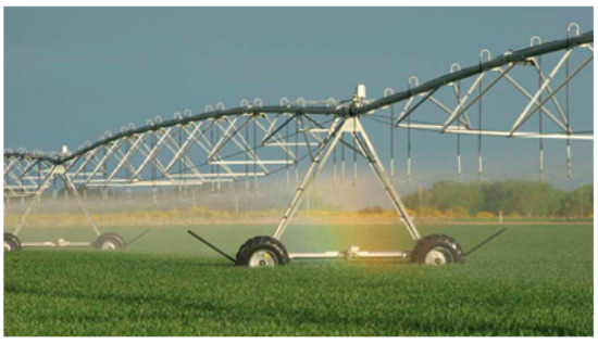
Figure 3.
A typical long moving irrigator.
With 45° reflection, the horizontal separation between transmitter and receiver units is 2h (nominally 4 m). In order that the reflection angle is sensibly constant, a design angular beam half-width of 5° was chosen, giving a design half-power “footprint” of width less than 1 m. Such a design is readily achieved using linear arrays of small speakers and microphones, resulting in a transmitter array and a receiver array, each of length 0.6 m.
The 2D intensity pattern on the ground can be calculated by summing the transmitted waves from each speaker allowing for distances (and correct phase) and for spherical spreading of the power. Assuming omnidirectional reflection from a diffusely reflecting surface, the power reaching each microphone can then be calculated, again allowing for distances and spherical spreading. Figure 4 shows the resulting predicted footprint sensitivity for recorded intensity, at a frequency of 3.4 kHz, with h = 2 m and with 6 speakers per array. The half-power width is 0.5 m along the direction between transmitter and receiver, and 2 m in the transverse direction. The sensitivity falls off rapidly from the central plateau.
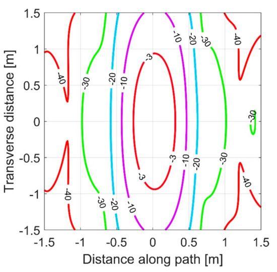
Figure 4.
Theoretical footprint sensitivity in dB for the transmitter and receiver both at a height of h = 2 m and a frequency of 3.4 kHz.
2.3. Temporal Resolution and Electrical Design
The oblique transmission path at 45° to the ground between the two masts of height h is of length 2(21/2h) and is well-defined using directional arrays. However, there is also a weaker direct-path horizontal transmission of length 2h. The path difference of 2(21/2 − 1)h corresponds to a propagation time difference of 5 ms for h = 2 m when the sound speed is 340 m s−1. Use of short pulses of duration less than 5 ms ensures that the direct and reflected signals can be separated. The pulse repetition rate was set at 15 pulses per second, which is more than three times the time taken for an entire pulse to travel the oblique path and ensures that there is no possibility of aliasing of reflections from any hard objects within a radius of 10 m.
For design and testing, the speakers were driven in parallel by a laptop-generated modulated signal via a 30 W audio amplifier. The microphones, also connected in parallel, were sampled by a data acquisition system controlled by the laptop. The system was powered by a battery, which can be maintained via a solar panel. For final operational use, a Raspberry PI with an appropriate acoustic add-on module and a graphics processing unit, would be adequate since fewer than 1024 samples need to be processed for each transmission at 44,100 samples per second. On this unit, the time taken to record 1024 samples at 44,100 samples per second would be 23 ms and the time required for data processing using a Fast Fourier Transform would be less than 0.2 ms [21].
3. Sensor Testing
A series of experiments were carried out to test the sensor in increasingly complex environments (e.g., presence of acoustic noise). The sensor was initially tested in a laboratory environment. The initial test provided an opportunity to further improve the performance of the sensor in the presence of acoustic noise such as from farm machinery. The results from the initial laboratory test are presented in Section 3.1. The sensor was then tested outside the laboratory first before testing it beneath a moving irrigator. Section 3.2 describes the results from an initial field test, whereas the results from a test beneath a moving irrigator are described in Section 3.3. Finally, the effects of pasture cover on the performance of the sensor are presented in the Section 3.4.
3.1. Initial Laboratory Investigation
Initial tests were completed in an anechoic chamber [22]. A tray of dimensions 285 mm by 385 mm was filled with 8.6 kg of dry soil to a depth of 75 mm. Water was added incrementally to the tray to give saturated soil and soil with a water overlayer. A linear array of seven speakers directed a short burst of sound onto the tray, which was surrounded by acoustic foam to absorb any sound extending beyond the tray edges. A single microphone 2 m from the speaker array center recorded sound reflected at 45°. Some results are shown in Figure 5. There is a clear increase in reflectivity with addition of water to the initially dry soil.
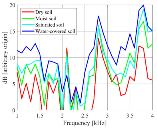
Figure 5.
Measured reflection from dry, moist, saturated, and water-covered soil.
Based on the initial trials, and to provide better performance in the presence of acoustic noise, the transmitted acoustic pulses were phase-encoded with a 13-bit Barker code. The coded pulse is generated by concatenation of 13 single sinusoidal wave cycles, with the amplitudes of cycles multiplied by 1, 1, 1, 1, 1, −1, −1, 1, 1, −1, 1, −1, 1, respectively. The phase changes per cycle means each pulse is 13 cycles of the base frequency, and pulse durations are 6.5 ms for 2 kHz to 3.25 ms for 4 kHz. The Barker code was chosen for further testing of the sensor so that good temporal separation is obtained between the oblique (reflected) path and the direct path signals. The reflected signal is cross-correlated (or matched filtered) with the Barker code pulse, and squared, to give a temporal resolution of 0.13/f or 0.065 ms at f = 2 kHz, so extending the pulse duration past 5 ms is not a problem. The result of the signal processing of these modulated pulses is to obtain an effective “compressed” pulse duration of 0.065 ms or a range resolution of 22 mm.
3.2. Initial Field Experiments
Initial field experiments were performed using a 0.45 m x 0.6 m tray of soil placed at ground level at the center of a frame upon which instrumentation was mounted. Tests conducted with acoustic foam covering the top edges of the soil tray showed that reflections from the tray edges were negligible. A manometer allowed the water level to be continuously varied. A downward facing 3D structured light camera (Intel RealSenseTM Depth Camera D415) viewed the earth-filled tray, so that topology and pooled water could be recorded. Processing of the 3D camera images allowed the soil surface topography to be quantified [22], which was of particular use when depressions were manually introduced and allowed to gradually fill with water
In the first set of experiments, the fraction α of the soil surface covered in water was estimated from 3D camera images [23,24] and compared with measured acoustic reflectance measured using pulses of frequency 2.5, 2.9, 3.3, 3.7, 4.1, and 4.5 kHz modulated as described above. Depressions were manually made in the soil surface and gradually filled with water. Figure 6 shows data from two different experiments. The first, shown in black, includes error bars calculated from the variation with frequency at each areal coverage. Results, when normalized to the maximum intensity at each frequency, were nearly independent of frequency. The curve in red on Figure 6 shows a much more extensive range of area coverage of water. The salient feature of these experiments is that there is a substantial, statistically significant, increase in reflectance up to a fractional cover of 40–60% and dropping off thereafter.
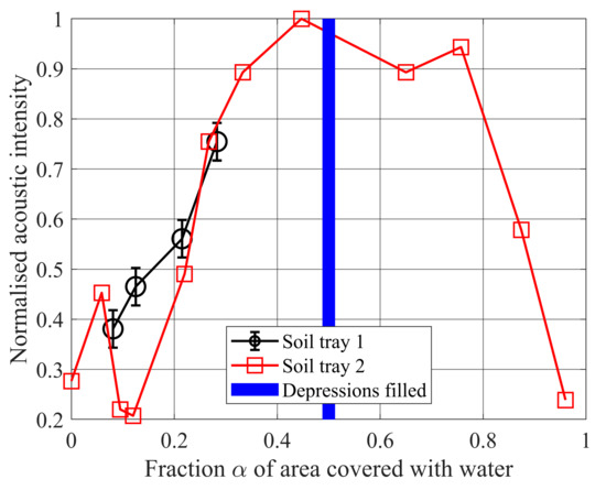
Figure 6.
Results from two experiments on wetted soil trays. The fraction of soil surface covered with water is estimated from 3D camera images. The black curve also shows error bars based on the standard deviation of intensities measured at each of the 6 transmission frequencies. The blue bar indicates the point at which depressions became full.
The sensor was further tested in a field setting on flat grassed farmland near Lincoln in the South Island of New Zealand (approximately 43°38′ S 172°28′ E). The set up comprised the speaker and microphone arrays, both mounted at 45° above a bounded runoff plot (1 m × 1 m). The downward facing 3D structured light camera viewed the bounded runoff plot, so that its topology could be recorded, including any pooled water. The measurements were progressively done from the soil surface having empty depressions to the state where all the soil surface depressions were completely filled with water. Results are shown in Figure 7, with error bars showing the variability with frequency. The general behavior is similar to that of the two tray experiments, although the peak in this case is at a lower fractional cover α.
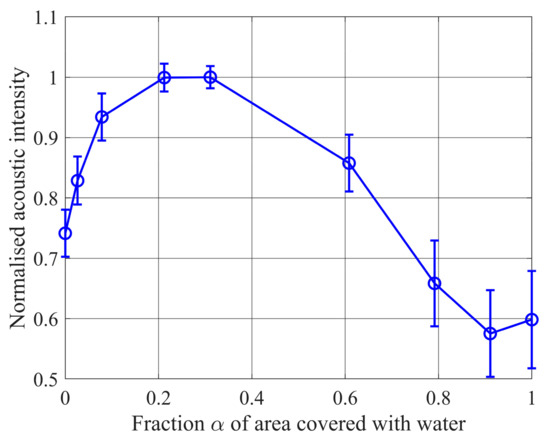
Figure 7.
Results from the runoff plot experiment.
3.3. Measurements Beneath an Irrigator
The measurements were carried out under a lateral move irrigator system in sheep farm (Figure 8) near Lincoln in the South Island of New Zealand (approximately 43° 38′ S 172° 28′ E). The irrigator moved over the top of the frame at its normal rate of translatation across the field; therefore, the same region of the ground was insonified continually during the observation period as the irrigation was applied. Measurements of areal water cover were not possible because of the grass cover, but the topsoil moisture (0–6 cm) was monitored at three locations using time domain reflectometry sensors (ML3 ThetaProbe, Delta-T Devices). A tipping bucket rain gauge (Rain Collector II, Davis Instruments Corporation, Hayward, CA 94545, USA, 0.2 mm per tip) was used to measure irrigation amount and intensity. Results are shown in Figure 9 where the error bars are from the variation across the six frequencies transmitted. Although the horizontal scale is different, behavior similar to that of the previous experiments is observed with a significant increase in reflectance up to a soil moisture of around 0.27 m3 m−3 and a drop thereafter.
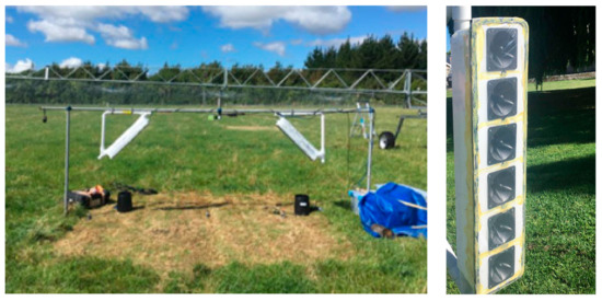
Figure 8.
The arrays (white rectangles) mounted on a small frame so that the mobile irrigator can pass over the instrument (left photograph), and a close-up of one of the arrays (right photograph). The height above ground at the center of each sloping array is h = 0.98 m, and the spacing between the two array centers is 2h = 1.96 m.
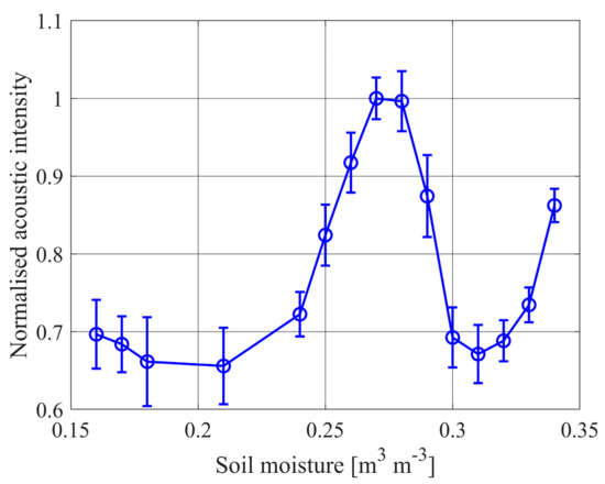
Figure 9.
Reflectance measurement dependence on soil moisture. The error bars are from the standard deviation of the measurements across the 6 transmitted frequencies.
3.4. Sensitivity to a Pasture Canopy
The ground impedance is known to depend on pasture coverage [14]. In order to evaluate the dependence of reflectivity on pasture cover, the frame shown in Figure 8 was mounted above three different areas of pasture. For each area, reflectance measurements were conducted over uncut pasture, pasture cut to mid-height, and pasture cut to close to the ground. Figure 10 shows results normalized to the “bare ground” intensities. The biomass dry matter was measured by collecting the cut pasture, drying it, and weighing. The biomass is given in kg per hectare in the figure caption.
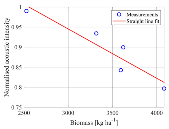
Figure 10.
Measured intensities normalized to the bare ground measurements and having different biomass.
These results indicate a significant pasture effect. There is some concern that the ground may have been compressed during the pasture cutting, and so measurements of pasture effect need to be repeated before the effect can be fully quantified. In addition to the effect of pasture cover, the effect of wetting of the pasture was investigated but found to be negligible.
4. Discussion
4.1. Acoustic Reflectance
The field measurements show a common behavior of an increase in reflectance with increasing water coverage α until a peak is reached. Further increasing water cover leads to a decrease in reflectance. However, modelling reflectance based on changes in porosity as the pores fill, or flow resistivity, shows a monotonic increase in reflectivity with increasing water content. A reason for this discrepancy may be that the traditional reflectance models are generally concerned with large scale sound propagation, whereas in the present case the interest is in only a 1 m2 area in which roughness features are potentially more important.
Consider a fraction α of the soil surface covered with water. The water is smooth and produces specular (mirror-like) reflection. The effect of soil surface roughness on reflection of an acoustic wave can be specified by the Rayleigh parameter kσh, where σh is the rms variation in soil surface height [25]. Measurements at the field sites described in Section 3 show that σh = 12–25 mm, so that for the frequency range used 0.4 < kσh < 1.9. For reflections, a surface is considered to be essentially flat if kσh < π/16 [24], so all soil surfaces described here are moderately rough for reflections. The fraction (1 − α) of surface presented by the soil is therefore assumed to reflect more omnidirectionally than the water surfaces. The overall reflectivity is
where Rsoil is the reflectivity of soil and Rwater is the reflectivity of water. The factor γ allows for the lower reception of specular reflected sound due to much of the divergent acoustic beam being reflected into angles which bypass the linear array of microphones.
R = (1 − α)Rsoil + αγRwater
The soil reflectance depends on moisture content and can be written as the sum of a dry soil reflectance term, Rdry, and a moisture-dependent term. The moisture-dependent term will increase with water fraction α because of water filling pores. Assume therefore that
Rsoil = Rdry + α dRsoil/dα.
Equation (3) can alternatively be considered as a first-order expansion of the dependency of Rsoil on α. The recorded acoustic intensity can be written as
I = GR.
The gain G, which includes the transmitter and receiver array sensitivities and the angular acoustic beam pattern, can be determined through experimental calibration. Combining (2), (3), and (4), the intensity dependence on water cover will have the form
I = I0 + αI1 + α2I2.
Results from the two soil tray experiments (shown in Figure 6) and from the runoff experiment (Figure 7) are reproduced in Figure 11 together with quadratic regressions based on the simple model in Equation (5). The quadratic regression shown in blue has a rms error of 0.17 and a coefficient of variation R2 = 0.65. The quadratic regression shown in red has a rms error of 0.08 and a coefficient of variation R2 = 0.83. The rms error for the red curve compares closely with the inherent mean measurement error of 0.05 shown in Figure 7. This implies that the simple model fully describes the observed behavior, to within measurement uncertainty.
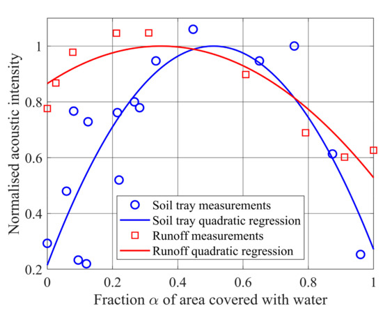
Figure 11.
Reflectance measurements from soil tray and runoff plot together with quadratic regressions based on the model.
The two regression curves in Figure 11 suggest quite different dry soil reflectivity. This is possibly because one regression curve was for when a tray was manually filled with soil, and the other curve was from a runoff plot experiment obtained under natural conditions.
4.2. Operational Implementation
The initiation of overland flow generally occurs at a critical value of connectivity, COF, the proportion of the soil surface that is connected via a water-filled pathway to an exit point of the field. Quantifying the development of COF during an irrigation event, therefore, is key to predicting the initiation of overland flow.
The experimental results and model described above relate observed acoustic reflectivity to the fraction α of the soil surface covered with water. Ghimire et al. 2020 [26] used a ponding and redistribution model to relate COF to α. They found that the average α required for establishing full hydrological connectivity increases with the increase in depressional storage capacity, indicating a significant link between α and overland flow connectivity.
The fraction of the soil surface covered with water, α, and hence COF can be estimated in real-time from acoustic reflectivity measurements based on inverting (5):
α = −{[I1/(2I2)]2 + (I − I0)/I2}1/2 − I1/(2I2).
From (6) the estimated uncertainties in regression parameters I0, I1, and I2, together with the uncertainties in measurements I shown in Figure 6 and Figure 7, can be used to estimate the uncertainty in real-time estimates of α. A conservative pulse repetition rate of 8 s−1 was used, with averaging of the acoustic signals over the duration of each α estimate. More realistically, the pulse transmission rate could be 100 pulses per second, giving improved estimation of α, and hence COF, from (5). Figure 12 shows the uncertainty σα in real-time operational estimation of α based on these considerations, as acoustic intensity increases with increasing irrigation. For example, from the runoff case in Figure 11 when α = 0.3, the estimation uncertainty would be σα = 0.086 or around ±30% of the true α. While this is quite a large uncertainty, the real-time decision making would be expected to be based on the trend of COF estimates which would smooth estimation variations.
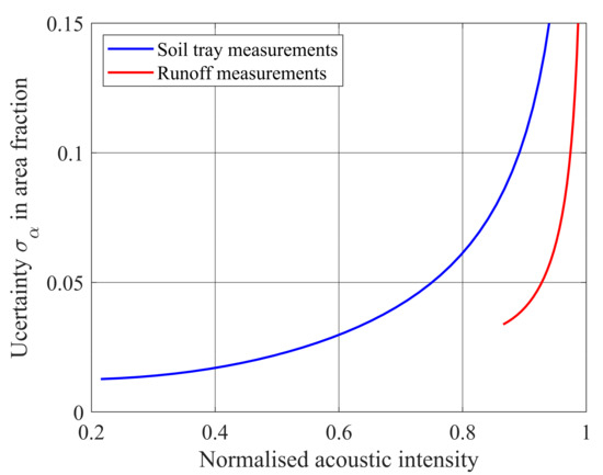
Figure 12.
Uncertainty in estimation of α for real-time operational monitoring of COF.
5. Conclusions
A relatively simple acoustic remote sensing instrument has been designed to allow real-time estimation of the extent of free surface water under an irrigation system. The instrument comprises two linear arrays, one for transmission and one for reception. The directionality of the arrays gives a well-defined footprint area on the ground beneath the instrument. The instrument has been mounted on a moving irrigator and can be solar powered and autonomous.
Laboratory and field measurements show that the measured acoustic reflectance increases in a statistically significant fashion up to the point where the fraction of surface covered with water is around 0.5. For further injection of water, the reflectivity decreases. A simple model is proposed to account for this observed behavior. It is proposed that the decrease in reflectivity is related to the change from diffuse reflection to specular reflection as the fraction of water surface increases. Within the measurement uncertainties, this model agrees with observations and has the potential to be developed so that the remote acoustic method can estimate surface free water for real-time irrigation control. There are effectively only three model parameters. These allow for an estimation of the point at which peak free water will occur. The instrumentation combined with the physical model provides the potential for real-time monitoring and control of irrigation systems to mitigate overland flow.
6. Patents
Snow, V., Bradley, S.G., Ghimire, C.P. Ground Surface Condition Sensing In Irrigation Systems. NZ750742, 15 February 2019 NZ754059, 30 May 2019. AgResearch/University of Auckland.
Author Contributions
Conceptualization, S.B. and V.S.; Formal analysis, S.B., C.G. and L.G.; Funding acquisition, S.B. and V.S.; Investigation, S.B. and C.G.; Methodology, S.B. and C.G.; Project administration, V.S.; Resources, S.B., C.G. and V.S.; Software, S.B., A.R., C.G. and L.G.; Supervision, S.B. and V.S.; Validation, S.B., A.R., C.G. and L.G.; Writing—original draft, S.B.; Writing—review and editing, S.B., C.G., L.G., S.L. and V.S. All authors have read and agreed to the published version of the manuscript.
Funding
This research was funded by the New Zealand Ministry of Business, Innovation and Employment via its Endeavour Smart Ideas contract C10X1708.
Acknowledgments
The authors are grateful for comments by Mostafa Sharifi of AgResearch Ltd. The manuscript benefited from the comments of two anonymous reviewers which are gratefully acknowledged.
Conflicts of Interest
The authors declare no conflict of interest. The funders had no role in the design of the study; in the collection, analyses, or interpretation of data; the writing of the manuscript, or in the decision to publish the results.
References
- Searchinger, T. Creating a Sustainable Food Future. World Resources Report; World Resources Institute: Washington, DC, USA, 2019; 564p, ISBN 978-1-56973-963-1. [Google Scholar]
- Laurenson, S.; Cichota, R.; Reese, P.; Breneger, S. Irrigation runoff from a rolling landscape with slowly permeable subsoils in New Zealand. Irrig. Sci. 2018, 36, 121–131. [Google Scholar] [CrossRef]
- Drewry, J.J.; McNeill, S.; Carrick, S.; Lynn, I.H.; Eger, A.; Payne, J.; Rogers, G.; Thomas, S.M. Temporal trends in soil physical properties under cropping with intensive till and no-till management. N. Z. J. Agric. Res. 2019, 1–22. [Google Scholar] [CrossRef]
- Houlbrooke, D.; Laurenson, S. Effect of sheep and cattle treading damage on soil microporosity and soil water holding capacity. Agric. Water Manag. 2013, 121, 81–84. [Google Scholar] [CrossRef]
- Xingming, Z.; Tao, J.; Xiaofeng, L.; Yanling, D.; Kai, Z. The temporal variation of farmland soil surface roughness with various initial surface states under natural rainfall conditions. Soil Tillage Res. 2017, 170, 147–156. [Google Scholar] [CrossRef]
- Moreno, R.G.; Alvarez, M.D.; Requejo, A.S.; Delfa, J.V.; Tarquis, A. Multiscaling analysis of soil roughness variability. Geoderma 2010, 160, 22–30. [Google Scholar] [CrossRef]
- Yang, J.; Chu, X. A new modeling approach for simulating microtopography-dominated, discontinuous overland flow on infiltrating surfaces. Adv. Water Resour. 2015, 78, 80–93. [Google Scholar] [CrossRef]
- Chu, X.; Yang, J.; Chi, Y.; Zhang, J. Dynamic puddle delineation and modeling of puddle-to-puddle filling-spilling-merging-splitting overland flow processes. Water Resour. Res. 2013, 49, 3825–3829. [Google Scholar] [CrossRef]
- Appels, W.M.; Bogaart, P.W.; van der Zee, S.E.A.T.M. Influence of spatial variations of microtopography and infiltration on surface runoff and field scale hydrological connectivity. Adv. Water Resour. 2011, 34, 303–313. [Google Scholar] [CrossRef]
- Cramond, A.J. Reflection of impulses as a method of determining acoustic impedance. J. Acoust. Soc. Am. 1984, 75, 382. [Google Scholar] [CrossRef]
- Laranja, R.A.; Budel, V.M.; Amorim, H.J.; Sobczyk, M.R.S. Experimental Evaluation of the Acoustic Impedance of Different Ground Types by Sound Propagation in Open-Air Environments. Adv. Mater. Res. 2014, 902, 185–191. [Google Scholar] [CrossRef]
- Horoshenkov, K.V.; Mohamed, M. Experimental investigation of the effects of water saturation on the acoustic admittance of sandy soils. J. Acoust. Soc. Am. 2006, 120, 1910. [Google Scholar] [CrossRef]
- Mohamed, M.; Horoshenkov, K.V. Airborne Acoustic Method to Determine the Volumetric Water Content of Unsaturated Sands. J. Geotech. Geoenviron. Eng. 2009, 135, 1872–1882. [Google Scholar] [CrossRef]
- Attenborough, K.; Bashir, I.; Taherzadeh, S. Outdoor ground impedance models. J. Acoust. Soc. Am. 2011, 129, 2806–2819. [Google Scholar] [CrossRef] [PubMed]
- Tarboton, D.G.; Bandaragoda, C.J.; Kaheil, Y.; Zachry, M.; Reed, W. An Online Module on Rainfall Runoff Processes; Civil and Environmental Engineering Faculty Publications: Logan, UT, USA, 2003; p. 2786. Available online: https://digitalcommons.usu.edu/cee_facpub/2786 (accessed on 27 October 2020).
- Taraldsen, G.; Jonasson, H. Aspects of ground effect modeling. J. Acoust. Soc. Am. 2011, 129, 47–53. [Google Scholar] [CrossRef] [PubMed]
- Brandão, E.; Lenzi, A.; Paul, S. A Review of the In Situ Impedance and Sound Absorption Measurement Techniques. Acta Acust. United Acust. 2015, 101, 443–463. [Google Scholar] [CrossRef]
- Adamo, F.; Andria, G.; Attivissimo, F.; Giaquinto, N. An Acoustic Method for Soil Moisture Measurement. IEEE Trans. Instrum. Meas. 2004, 53, 891–898. [Google Scholar] [CrossRef]
- Cramond, A.J. Effects of moisture content on soil impedance. J. Acoust. Soc. Am. 1987, 82, 293. [Google Scholar] [CrossRef]
- Rossing, T. Springer Handbook of Acoustics; Springer Science & Business Media: New York, NY, USA, 2007. [Google Scholar]
- Sabarinath, S.; Shyam, R.; Aneesh, C.; Gandhiraj, R.; Soman, K.P. Accelerated FFT Computation for GNU Radio Using GPU of Raspberry Pi. Smart Intell. Comput. Appl. 2014, 32, 657–664. [Google Scholar]
- Radionova, A.; Ghimire, C.P.; Grundy, L.; Laurenson, S.; Bradley, S.; Snow, V. Acoustic Remote Sensing for Irrigation Systems Control in Agriculture. In Proceedings of the 23rd International Congress on Acoustics, Aachen, Germany, 9–13 September 2019; pp. 2870–2877. [Google Scholar]
- Ghimire, C.P.; Appels, W.M.; Grundy, L.; Rtichie, W.; Bradley, S.; Snow, V. Predicting the initiation of overland flow from relatively flat agricultural field using surface water coverage. J. Hydrol. 2020. accepted. [Google Scholar]
- Grundy, L.; Ghimire, C.; Snow, V. Characterisation of soil micro-topography using a depth camera. MethodsX 2020, 101144. [Google Scholar] [CrossRef]
- Pinel, N.; Bourlier, C.; Saillard, J. Degree of roughness of rough layers: Extensions of the Rayleigh roughness criterion and some applications. Prog. Electromagn. Res. B 2010, 19, 41–63. [Google Scholar] [CrossRef]
- Ghimire, C.P.; Snow, V.O.; Bradley, S.; Grundy, L. Proximal Remote Sensing to Quantify Plot-Scale Overland Flow Connectivity. In EGU General Assembly Conference Abstracts; European Geophysical Union: Munich, Germany, 2020. [Google Scholar] [CrossRef]


Publisher’s Note: MDPI stays neutral with regard to jurisdictional claims in published maps and institutional affiliations. |
© 2020 by the authors. Licensee MDPI, Basel, Switzerland. This article is an open access article distributed under the terms and conditions of the Creative Commons Attribution (CC BY) license (http://creativecommons.org/licenses/by/4.0/).