Abstract
Accurate vegetation detection is important for many applications, such as crop yield estimation, land cover land use monitoring, urban growth monitoring, drought monitoring, etc. Popular conventional approaches to vegetation detection incorporate the normalized difference vegetation index (NDVI), which uses the red and near infrared (NIR) bands, and enhanced vegetation index (EVI), which uses red, NIR, and the blue bands. Although NDVI and EVI are efficient, their accuracies still have room for further improvement. In this paper, we propose a new approach to vegetation detection based on land cover classification. That is, we first perform an accurate classification of 15 or more land cover types. The land covers such as grass, shrub, and trees are then grouped into vegetation and other land cover types such as roads, buildings, etc. are grouped into non-vegetation. Similar to NDVI and EVI, only RGB and NIR bands are needed in our proposed approach. If Laser imaging, Detection, and Ranging (LiDAR) data are available, our approach can also incorporate LiDAR in the detection process. Results using a well-known dataset demonstrated that the proposed approach is feasible and achieves more accurate vegetation detection than both NDVI and EVI. In particular, a Support Vector Machine (SVM) approach performed 6% better than NDVI and 50% better than EVI in terms of overall accuracy (OA).
1. Introduction
The normalized difference vegetation index (NDVI) [1,2] has been applied to the monitoring of land use and land cover change [3] drought, desertification [4], desertification [5], soil erosion [6], vegetation fires [7], biodiversity and conservation [8], and soil organic carbon (SOC) [9]. Although NDVI has been widely used due to its simplicity, its accuracy still has room for improvement. Liu and Huete [10] proposed an enhanced vegetation index (EVI) that incorporates the blue band into the calculation. Although the EVI performs better than the NDVI in some applications, it was shown in [11] that it is more sensitive to topographic conditions than the NDVI.
Land cover classification using multispectral and hyperspectral images [12,13,14,15,16] has been widely used for urban growth monitoring, land use monitoring, flood and fire damage assessment, etc. In recent years, Laser imaging, Detection, and Ranging (LiDAR) has also been used for land cover classification. There are many land cover classification methods in the literature, including conventional and deep learning methods. In many land cover classification papers, researchers use all of the multispectral and hyperspectral bands for classification. Recently, there have been some investigations [17,18,19] that only use a few bands such as RGB and NIR bands, and yet can still achieve reasonable classification accuracy. In [17], it was found that synthetic bands using Extended Multi-attribute Profiles (EMAP) [20,21,22,23] can help improve the land classification performance quite significantly.
In some applications, such as construction planning, land surveying, etc., an accurate digital terrain model (DTM) is essential [24]. However, the terrain may be covered by vegetation (trees, shrubs, grass). Although digital surface model (DSM) obtained by radar or LiDAR can provide a general idea of the terrain, the presence of vegetation such as trees conceals the actual terrain elevation. In some past research in construction surveying [24], people have used NDVI to detect the vegetation, followed by a trimming step that removes the elevation due to trees and grass. Few studies carried out some quantitative comparisons of normalized difference vegetation index (NDVI) with other methods provided, except [18]. In [18], NDVI only method achieved 75% accuracy whereas some alternative methods-based machine learning and deep learning yielded 10% better accuracy. In this paper, a Support Vector Machine (SVM) approach performed 6% better than NDVI and 50% better than EVI in terms of overall accuracy (OA). Moreover, based on our sponsor’s (US Dept. of Energy) independent assessment, the NDVI approach is not accurate enough and urged us to develop some sophisticated land cover classification-based methods to accurately detect vegetation.
We would like to raise several important research questions in the land cover classification approach to vegetation detection. First, will the vegetation detection performance be improved if hyperspectral images are used instead of using only the RGB and NIR bands? This is an important question because, if the use of hyperspectral data does not improve the vegetation detection, then it will be better to only use RGB and NIR bands, which can be acquired inexpensively. Second, if only RGB and NIR bands are used, will the vegetation detection performance be improved with EMAP enhanced bands? This question is important, because EMAPs have been found to yield good land cover classification performance before. It will be interesting to investigate whether or not EMAPs can help the vegetation detection as well. Third, since there are many classification algorithms in the literature, does there exist any simple and efficient algorithms that can yield good vegetation detection performance? Fourth, if the classification approach is better than NDVI or EVI approaches, how much gain will that be? The quantification will help decision makers to decide on whether to deploy the land classification approach to vegetation detection. Fifth, in some cases, LiDAR data may be available. Will LiDAR help the vegetation detection performance?
In this paper, we propose a new vegetation detection approach based on land classification. The approach is very simple, intuitive, and uses only RGB and NIR bands. We first apply proven land cover classification algorithms to RGB and NIR bands to classify the land cover types. The resulting classification maps are then grouped into vegetation and non-vegetation categories. Experimental results showed that the proposed approach is highly accurate and practical. In our investigations, we also provide answers to the five questions raised earlier.
Our paper focuses on an application that demands higher vegetation detection accuracy and also that training data are available. In such application scenarios, it is necessary to call for more accurate vegetation detection approaches. The contributions of our paper are to answer those questions raised earlier and are as follows:
- Although hyperspectral data have been used for various land cover classification applications, our experiments showed that the vegetation detection performance using hyperspectral data did not yield better results than those obtained using only the RGB and NIR bands.
- Although the use of an EMAP enhanced dataset does help the land cover classification, our experiments demonstrated the EMAP enhanced dataset does not improve the vegetation detection performance. This is counter intuitive, and we will address this important observation in Section 3.
- Using a benchmark dataset, our experiments demonstrated that the land classification approach using only red-green-blue (RGB) and near infrared (NIR) bands can perform better than the NDVI and EVI approaches for this dataset. In particular, a Support Vector Machine (SVM) approach performed 6% better than NDVI and 50% better than EVI in terms of overall accuracy (OA).
- Our results demonstrated that, if LiDAR data are available, the vegetation detection performance can be improved slightly.
2. Methods and Data
2.1. Land Cover Classification Methods
For land cover classification, there are pixel-based and object-based methods. In this paper, we focus on pixel-based methods because the 2013 Institute of Electrical and Electronic Engineers (IEEE) GRSS Data Fusion Contest dataset [25] only contains training and testing samples in pixels.
We applied nine pixel-based classification algorithms that have been widely used in hyperspectral images, including Matched Signature Detection (MSD), Adaptive Subspace Detection (ASD), Reed-Xiaoli Detection (RXD), and their kernel versions, and also Sparse Representation (SR), Joint SR (JSR), and Support Vector Machine (SVM) to the IEEE dataset [25] for land cover classification. These algorithms are detailed in [26] and short descriptions of them can also be found in [17]. For completeness, we include some brief descriptions for each method below. In addition, we also include a deep learning-based approach for land cover classification.
2.1.1. Matched Subspace Detection (MSD)
In MSD [26], there are two separate hypotheses: H0 (target absent) and H1 (target present) which are defined as:
where T and B are the orthogonal matrices that span the subspace of the target and background/non-target, θ and are the unknown vectors that account for the various different corresponding column vectors of T and B, respectively, and n represents random noise. A generalized likelihood ratio test (GLRT) to predict whether a specific pixel will be a target or background pixel is given by:
where , .
The reason that we chose MSD as one of the nine methods is because MSD has been proven to work well in some hyperspectral target detection applications [26].
2.1.2. Adaptive Subspace Detection (ASD)
ASD [26] has a very similar process to MSD with a slightly varying set of hypotheses:
where U is the orthogonal matrix, whose column vectors are eigenvectors of the target subspace, θ is the unknown vector whose entries are coefficients for the target subspace, and n is the random Gaussian noise. Those equations are then solved in order to create a similar GLRT to MSD. The classification is performed for each class first and the final decision is made by picking the class label that corresponds to the maximum detection value at each pixel location.
Similar to MSD, we adopted ASD simply because it has been proven to work quite well in target detection with hyperspectral images [26,27].
2.1.3. Reed-Xiaoli Detection (RXD)
RXD [28] is normally used for anomaly detection and it is simple and efficient. For land cover classification, RXD follows the same procedure as MSD and ASD, using H0 (target absent) and H1 (target present) hypotheses in its formulation and combining them to generate a GLRT. The background pixels come from training samples to detect pixels in class i. That is, RXD can be expressed as:
where r is the test pixel, μb is the estimated sample mean of the background classes, and Cb is the covariance of the training samples in the background classes.
The kernel versions of each of the above methods—ASD, MSD, and RXD—all follow a similar fashion.
2.1.4. Kernel MSD (KMSD)
In [26], it was demonstrated that KMSD has a better performance than MSD. In KMSD, the input data have been implicitly mapped by a nonlinear function Φ into a high dimensional feature space F. The detection model in F is then given by:
where the variables are defined in [26]. The kernelized GLRT for KMSD can be found in Equation (9) of [26].
2.1.5. Kernel ASD (KASD)
Similar to KMSD, KASD [26] was also adopted in our investigations because of its good performance in [26]. In KASD, similar to KMSD, the detection formulation can be written as:
The various variables are defined in [26]. The final detector in kernelized format can be found in Equation (30) of [26].
2.1.6. Kernel RXD (KRXD)
In KRXD, every pixel is transformed to a high dimensional space via a nonlinear transformation. The kernel representation for the dot product in feature space between two arbitrary vectors and is expressed as:
A commonly used kernel is the Gaussian radial basis function (RBF) kernel:
where c is a constant and x and y are spectral signatures of two pixels in a hyperspectral image. The above kernel function is based on the well-known kernel trick that avoids the actual computation of high dimensional features and enables the implementation of KRXD. Details of KRXD can be found in [28,29].
2.1.7. Sparse Representation (SR)
In [30], we applied SR to detect soil due to illegal tunnel excavation. It was observed that SR was one of the highest performing methods. We also included SR in this paper because of the above. SR exploits the structure of only having a few nonzero values by solving the convex -norm minimization problem:
where is defined as the number of non-zero rows of S, the signature values of a given pixel, is a pre-defined maximum row-sparsity parameter, q > 1 is a norm of matrix S that encourages sparsity patterns across multiple observations, and D is the dictionary of class signatures.
2.1.8. Joint Sparse Representation (JSR)
Similar to SR, JSR was used in our earlier study in soil detection [30]. Although JSR is more computationally demanding, it exploits neighborhood pixels for joint land type classification. In JSR, 3 × 3 or 5 × 5 patches of pixels are used in the S target matrix. It is the same equation as Equation (13), but with an added dimension to S that accounts for each pixel within whatever patch size is used. Details of the mathematics can be found in [30].
2.1.9. Support Vector Machine (SVM)
An SVM is a general architecture that can be applied to pattern recognition and classification [31], regression estimation and other problems, such as speech and target recognition. An SVM can be constructed from a simple linear maximum margin classifier that can be trained by solving a convex quadratic programming problem with constraints.
2.1.10. Our Customized Convolutional Neural Network (CNN)
In recent years, deep learning-based methods have attracted a lot of attention in remote sensing applications. See [32,33,34,35] and references therein. Some exhaustive reviews were given in [32,33]. In this paper, we used the same structure that was used in our previous work [36]. Only the filter size in the first convolution layer was changed accordingly to be consistent with the input patch sizes. This CNN model has four convolutional layers with various filter sizes and a fully connected layer with 100 hidden units as shown in Figure 1. When we designed the network, we tried different configurations for the number of layers and the size of each layer, and selected the one that provided the best results. We did this for all the layers (convolutional and FC layers). The choice of “100 hidden units” is the outcome of our design studies. This model was also used for soil detection due to illegal tunnel excavation in [37]. Each convolutional layer utilizes the Rectified Linear Unit (ReLu) as activation function. The last fully connected layer uses the SoftMax function for classification. We added dropout layer for each convolutional layer with a dropout rate of 0.1 to mitigate overfitting [38]. It should be noted that the network size changes depending on the input size. In Figure 1, the network should be the same for 5 × 5 than for 7 × 7, the only difference would be that the first layer is deleted. For 3 × 3, the first 2 layers are deleted. The number of bands (N) in the input image can be any integer numbers. In the experiments, we found that 5 × 5 patch size gave the best performance.

Figure 1.
Our customized Convolutional Neural Network (CNN) model.
2.2. NDVI
The methods in Section 2.1 were also compared against the Normalized Difference Vegetation Index (NDVI) method. NDVI is simply a ratio of [1]
where R and NIR denote the red and near infrared bands. The values that correspond to vegetation for NDVI are inclusively between −1 and 1. The values that correspond to non-vegetation are less than 0.
2.3. Enhanced Vegetation Index (EVI)
The EVI is defined as [10]
where G = 2.5, C1 = 6; C2 = 7.5; L = 1. The values that correspond to vegetation for EVI are inclusively between −1 and 1. The values that correspond to non-vegetation are less than 0. It was demonstrated that EVI has some advantages over NDVI in some applications [10].
2.4. EMAP
Mathematically, given an input grayscale image and a sequence of threshold levels , the attribute profile (AP) of is obtained by applying a sequence of thinning and thickening attribute transformations to every pixel in .
The EMAP of is then acquired by stacking two or more APs while using any feature reduction technique on multispectral/hyperspectral data, such as purely geometric attributes (e.g., area, length of the perimeter, image moments, shape factors), or textural attributes (e.g., range, standard deviation, entropy) [20,21,22,23].
In this paper, the “area (a)” and “length of the diagonal of the bounding box (d)” attributes of EMAP [39] were used. For the area attribute of EMAP, two thresholds used by the morphological attribute filters were set to 10 and 15. For the Length attribute of EMAP, the thresholds were set to 50, 100, and 500. The above thresholds were chosen based on experience, because we observed them to yield consistent results in our experiments. With this parameter setting, EMAP creates 11 synthetic bands for a given single band image. One of the bands comes from the original image.
EMAP has been used in hyperspectral image processing before. More technical details and applications of EMAP can be found in [20,21,22,23]. In fact, in [25,40], EMAP has been used for land cover classification before. One key difference between the above references and our approach here is that we applied EMAP to only RGB+NIR and RGB+NIR+LiDAR, whereas the above methods all used the original hyperspectral data.
2.5. Data
From the IEEE GRSS Data Fusion package [25], we obtained the hyperspectral image of the University of Houston area, the ground truth land cover information for the training and test pixels and the LiDAR data of the same area. The instruments used to collect the dataset are a hyperspectral sensor and a LiDAR sensor. The hyperspectral data contain 144 bands that range in wavelength from 380–1050 nm, with a spatial resolution of 2.5 m. Each band has a spectral width of 4.65 nm. The LiDAR data contain elevation information with a resolution of 2.5 m. The LiDAR sensor has a laser wavelength in three channels of 1550 nm, 1064 nm, and 532 nm with an operating altitude from 300 to 2500 m. The vertical accuracy is between 5–15 cm and the horizontal accuracy is a factor of the altitude at 1/5500 × altitude.
Table 1 displays the number of training and testing pixels per class. Figure 2 below shows the Houston area with the validation classifications for the test data set that is used to compare and determine the overall accuracy.

Table 1.
Number of pixels per class in the IEEE Geoscience and Remote Sensing Society (GRSS) data.

Figure 2.
Color image for the University of Houston area with training and testing pixels. On the right-hand side, there is a shadow area due to cloud. The land cover classification accuracy suffers in that area.
The predetermined training data set includes 2832 pixels and the testing data included the remaining 12,197 pixels from the University of Houston dataset.
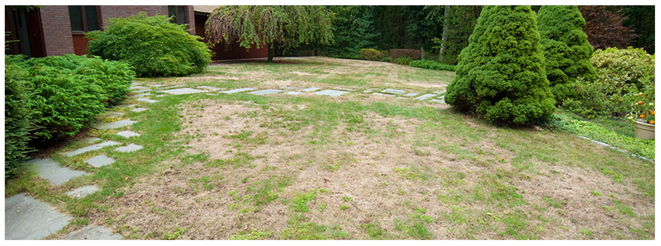
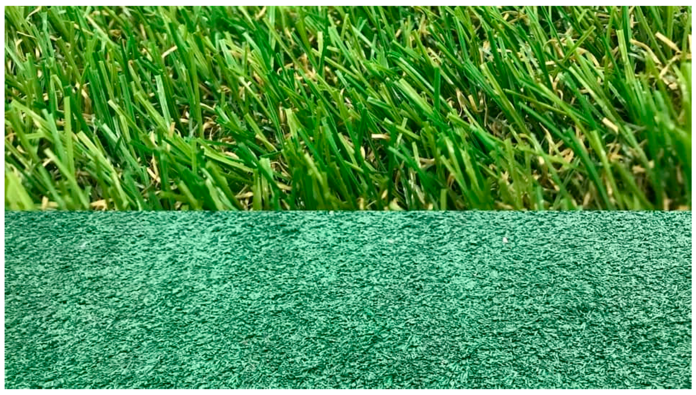
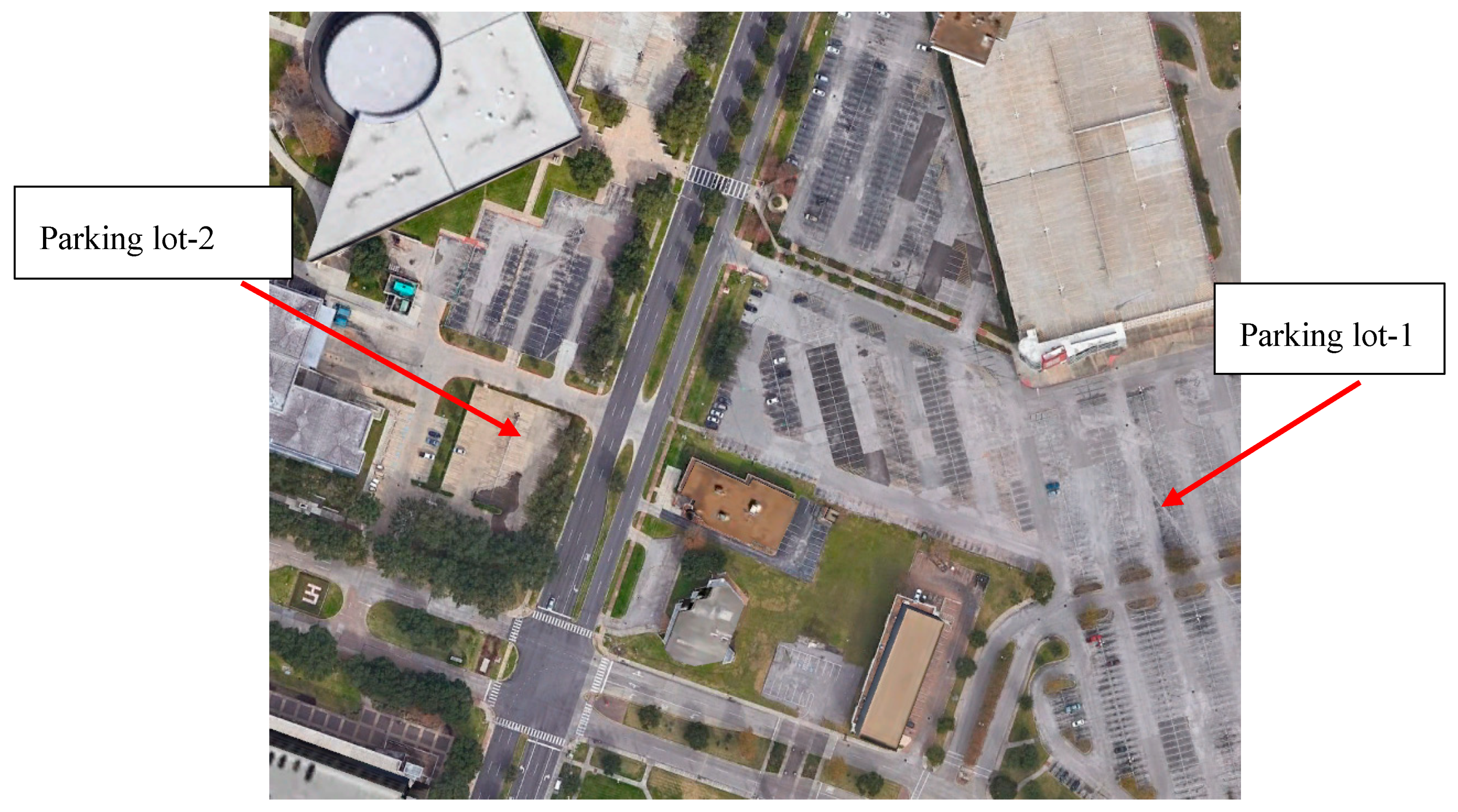
Some of the land cover classes in Table 1 may need some further explanations. Stressed grass differs from healthy grass since it is not watered enough and has brown spots whereas healthy grass is all green with no brown spots. An example picture showing stressed grass can be seen in Figure 3. The differences between synthetic and normal grasses can be clearly seen in Figure 4. Assuming that some of the building structures in the U. of Houston campus did not change, we looked at the same geographical site from Google Earth and we identified a number of ground truth pixels for “Parking lot-1” and “Parking-lot2” type land covers. The differences between the two parking lot types can be examined in the following screenshot in Figure 5. The materials that form these two types of parking lots seem to be quite different. Moreover, assuming that some of the building structures did not change, we looked at the same geographical site from Google Earth and we identified a number of ground truth pixels for “Residential” and “Commercial” type land covers in the IEEE dataset. A screenshot showing some of these locations using these ground truth pixels for these two land covers can be both seen in the Google Earth image and the hyperspectral dataset in Figure 6 to better visualize how these two land cover types differ. The other remaining land cover types, such as water, trees, soil, tennis courts, roads, etc., are self-explanatory.

Figure 3.
A picture showing stressed grass.
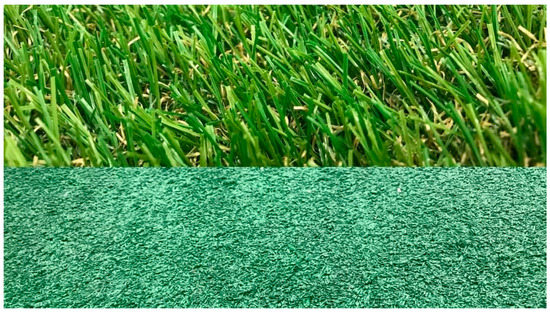
Figure 4.
Artificial grass (bottom) vs. real grass (top).

Figure 5.
Differences between Parking lot-1 and Parking lot-2 in the IEEE dataset can be better observed in Google Earth image for the same area.
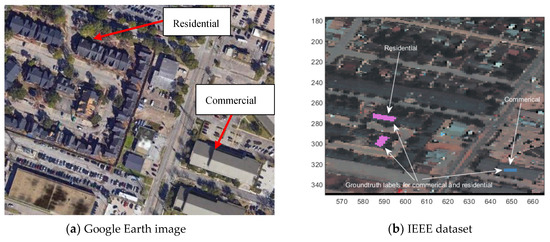
Figure 6.
Residential and commercial land cover examples in the hyperspectral dataset and corresponding Google Earth image. (a) Google Earth image; (b) IEEE dataset.
There are six datasets used for analysis in this paper, as shown in Table 2. The first group is the RGB (band # 60, 30, 22 in the hyperspectral data) and the NIR band (band #103). The other datasets are self-explanatory.

Table 2.
Dataset labels and the corresponding bands.
3. Vegetation Detection Results
For the six datasets mentioned in Section 2.5, we will present the land cover classification results using 10 algorithms mentioned in Section 3.1. We will then present the vegetation classification results in Section 3.2 by using 12 methods. Some interesting observations and explanations are then summarized in Section 3.3.
3.1. Fifteen-Class Land Cover Classification Results
There are 15 land cover types in the IEEE data. Here, we present land cover classification results using the 10 algorithms. The overall accuracy (OA) and average accuracy (AA) values obtained using six datasets are summarized in Table 3 and Table 4, respectively, for the conventional methods as well as for the deep learning CNN method. Overall accuracy is the total number of correct classifications across all classes divided by the total number of pixels. Average accuracy is the sum of each classes accuracy in the dataset divided by the total number of classes. We have the following observations:

Table 3.
Overall accuracy (OA) of 15-class classification in percentage of each method and band combination. Red highlighted numbers indicate the best accuracy for each method and bold numbers indicate the best accuracy for each dataset.

Table 4.
Average accuracy (AA) of 15-class classification in percentage of each method and band combination. Red highlighted numbers indicate the best accuracy for each method and bold numbers indicate the best accuracy for each dataset.
- SVM and JSR perform better than other conventional methods.
- CNN performs the best in most cases.
- Land cover classification with EMAP (DS-44 and DS-55) improves over those without EMAP (DS-4 and DS-5).
- Hyperspectral data (DS-144) do not perform better than EMAP cases. We will offer some explanations on why this is the case.
- LiDAR (DS-5, DS-55, and DS-145) helps land classification in some cases, but not always.
3.2. Two-class Vegetation Classification Results
We now recast the vegetation detection problem into a two-class classification setting, where all vegetation classes are grouped into vegetation and the remaining classes into non-vegetation. This means combining the three land covers shown in Table 1 as vegetation—which are two versions of grass (healthy and stressed), and also trees—and the other 12 classes as non-vegetation, those being synthetic grass, soil, water, residential, commercial, road, highway, railway, parking lot 1, parking lot 2, tennis court, and running track. It should be noted that synthetic grass has the same appearance in terms of color and texture as real grass but was not considered as vegetation. The OA and AA results for two-class classification results are shown in Table 5 and Table 6. For some datasets, accuracies spike for each method with some standard methods (ASD, MSD, RXD) nearing OA values of 95%. The kernel methods also see drastic improvements with a majority resulting in 90% accuracy or higher for those datasets (DS-44, DS-55, DS-144, DS-145) as can be seen in Table 5. The best in both cases is MSD with the 55-band version returning 94.77% accuracy and KMSD’s 44-band case returning a value of 99.40% only missing 78 pixels out of 12,197.

Table 5.
Overall accuracy (OA) accuracies of two-class classification in percentage for six datasets using 11 vegetation detection algorithms. Red highlighted numbers indicate the best accuracy for each method and bold numbers indicate the best accuracy for each dataset.

Table 6.
Average accuracy (AA) accuracies in percentage of two-class classification for six datasets using 11 vegetation detection algorithms. Red numbers indicate the best accuracy for each method and bold numbers indicate the best accuracy for each dataset.
The objective of our investigation was mainly to compare the performances of all the investigated methods with the NDVI and EVI techniques. In this setting, SVM using RGB and NIR bands (DS-4: four bands) without EMAP surprisingly provided an overall accuracy of 99.54% whereas the NDVI technique’s overall accuracy was 93.74%. SVM with four bands also exceeded the performance of SVM when using all 144 bands which was 96.66%. In the two-class setting, we also observed that EMAP improved the accuracies for several methods but SVM was not among them.
The LiDAR band also slightly helped the SR performance to reach 98.29%, but the gain is about 0.77%. In other methods, the LiDAR band helped more drastically, for KMSD the improvement is a more substantial 7.08%, but not always, as is seen with MSD where the reduction in accuracy is 8.88%.
For two-class classification results, CNN did not yield the best performance. We think that this is because CNN has good intra-class classification performance, but not necessarily good performance for inter-classification. We have some further explanations in Section 3.3.
For completeness, 2 × 2 confusion matrices of vegetation and non-vegetation of all the nine conventional algorithms and six datasets are shown in Table 7, Table 8 and Table 9. Table 10 contains the results for the deep learning method, CNN. Because these results are much more compact than 15 × 15 confusion matrices, they can easily be included in the body of this paper.

Table 7.
Standard methods (ASD, MSD, RXD) veg vs. non-veg confusion matrices. GT means ground truth.

Table 8.
Kernel methods (KASD, KMSD, KRXD) veg vs. non-veg confusion matrices.

Table 9.
Other methods (SR, JSR, SVM) veg vs. non-veg confusion matrices.

Table 10.
Deep learning method (CNN) veg vs. non-veg confusion matrices.
The confusion matrices for the vegetation detection results (vegetation vs. non-vegetation) in Table 8, Table 9 and Table 10 using the 10 algorithms can now be compared with the NDVI and EVI results. Table 11 shows the results for NDVI. Given the quick computation times of these methods and that they do not need any training data, we conclude that the resulting percentages for NDVI are quite good. With an overall accuracy of 93.74%, NDVI beats 23 of the 45 scenarios, where one of the best overall accuracies, 99.54%, comes from the SVM case using four bands. However, NDVI does have its limitations, specifically that it can only differentiate between vegetation and non-vegetation and it cannot classify different types of vegetation. In some cases, differentiating trees from grass is important for construction surveying. The EVI results are shown in Table 12. The detection results for EVI are not good for this dataset even though EVI may have better performance than NDVI in other scenarios [11].

Table 11.
NDVI method confusion matrix. OA: 93.74%; AA: 91.62%.

Table 12.
EVI confusion matrix. OA: 49.74%; AA: 57.96%.
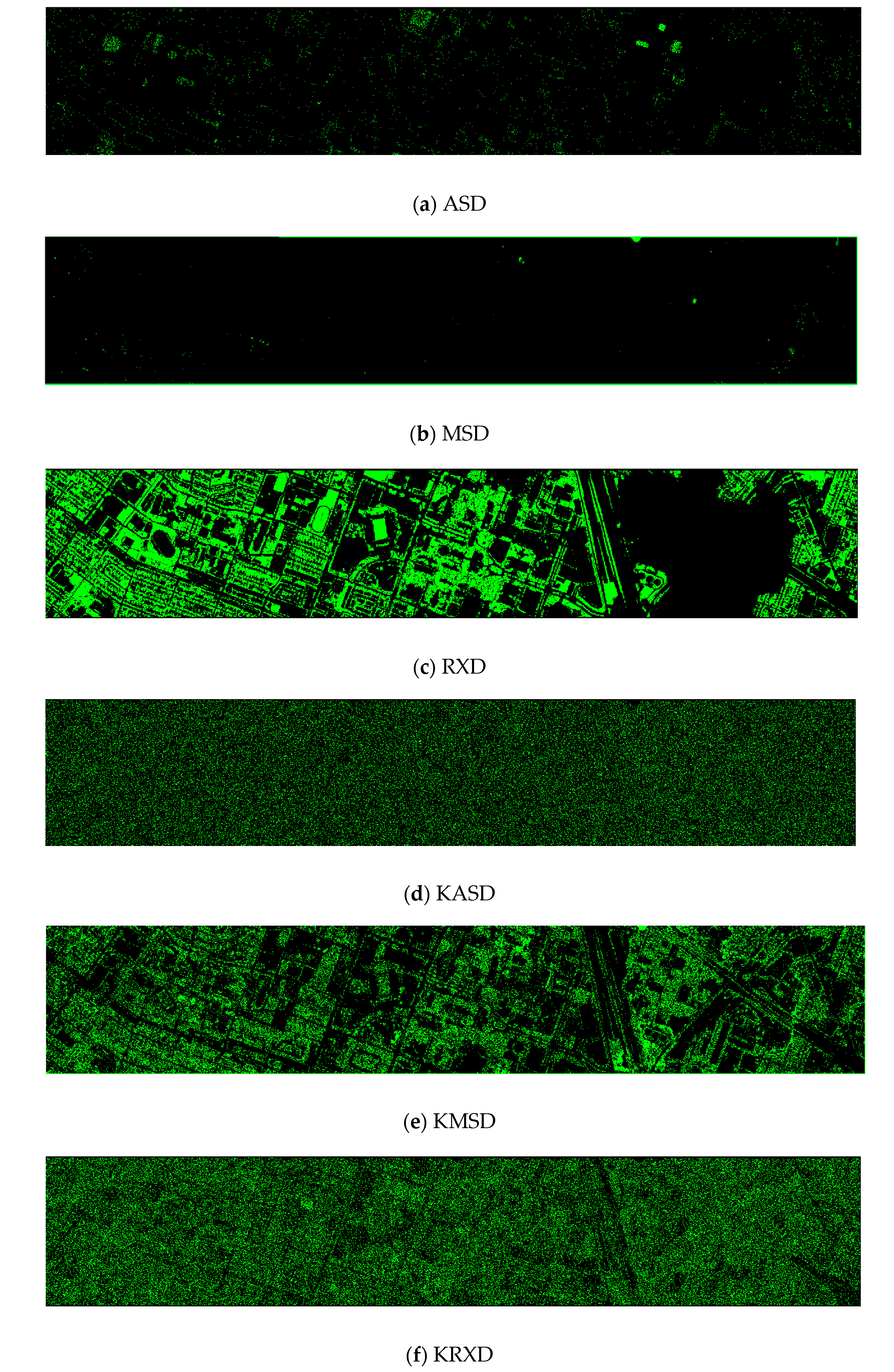
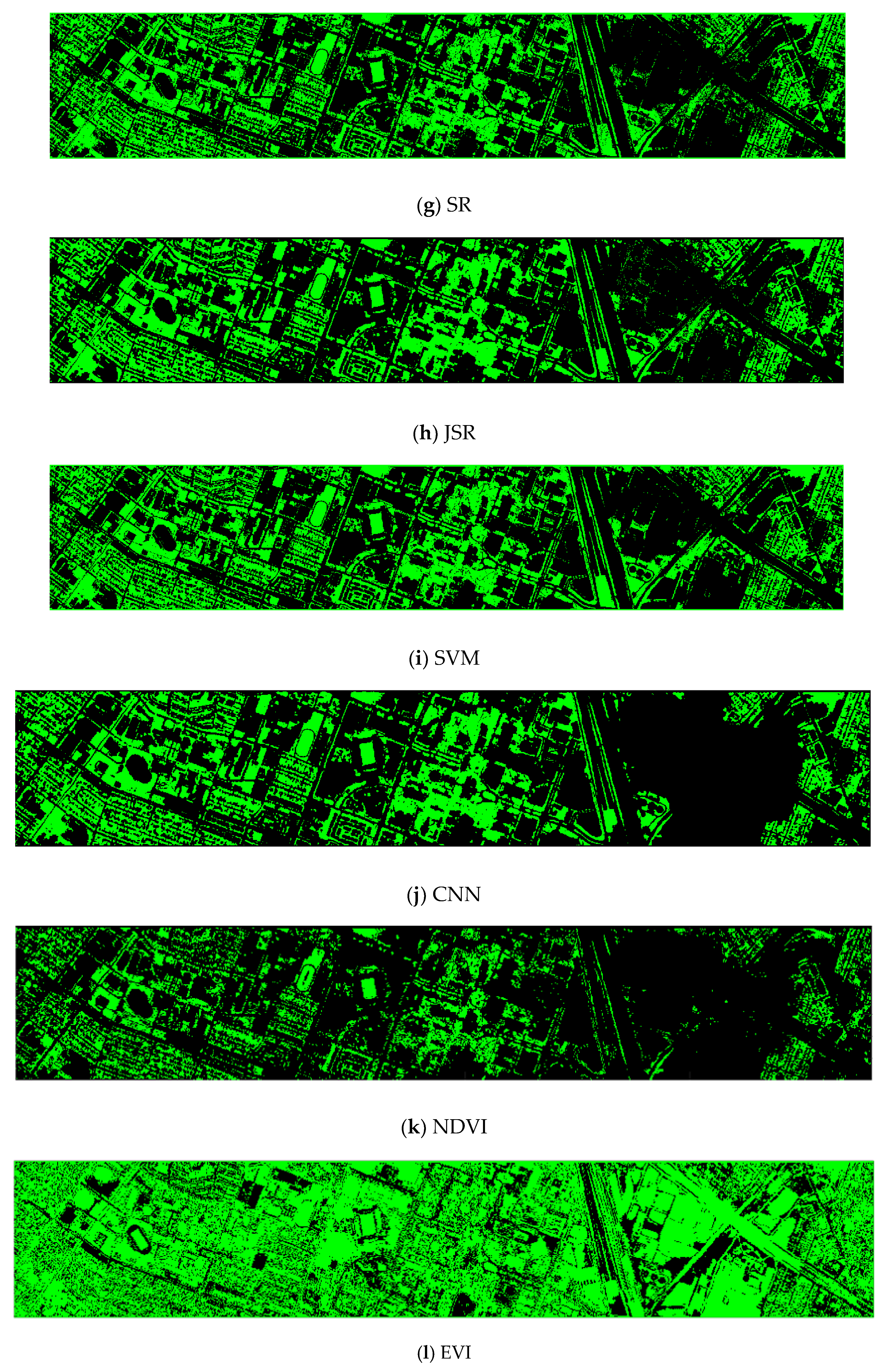
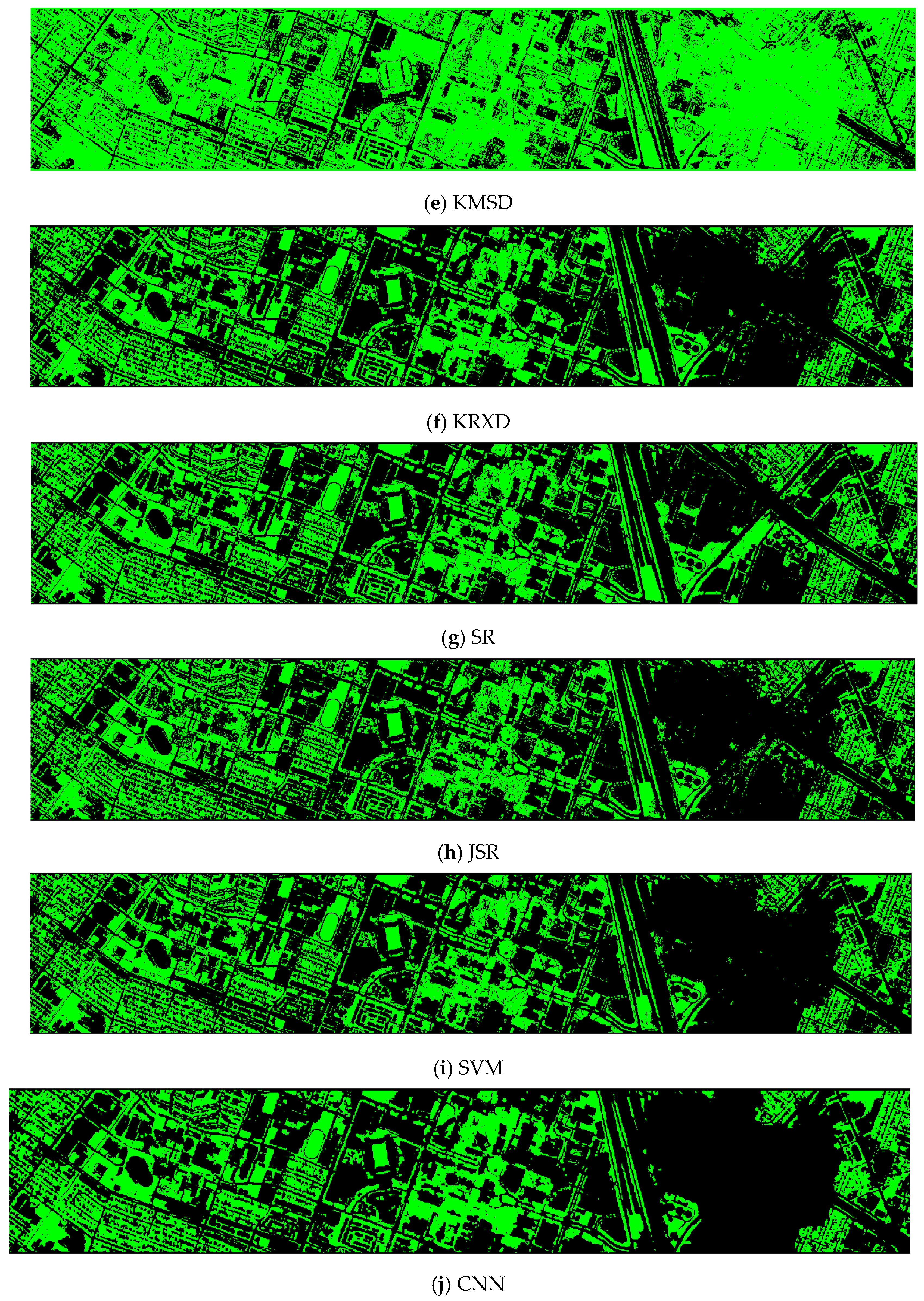
Finally, we would like to include some vegetation detection maps using different methods. Figure 7 shows the detection maps for the 4-band case. There are twelve maps, including ASD, MSD, RXD, KASD, KMSD, KRXD, SR, JSR, SVM, CNN, NDVI, and EVI. It can be seen that ASD, MSD, KASD, KRXD maps are not good. EVI has more false positives and NDVI has more missed detections. SR, JSR, SVM, and NN have comparable performance. Vegetation maps for DS-5, DS-44, DS-45, DS-144, and DS-145 can be found in Figure A1, Figure A2, Figure A3, Figure A4 and Figure A5, respectively in the Appendix A.
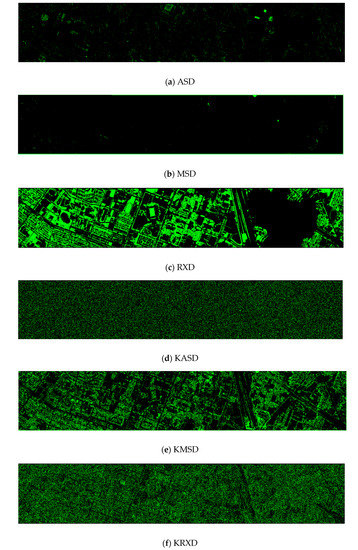
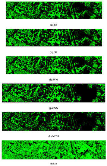
Figure 7.
Vegetation detection maps using eleven approaches. Green indicates vegetation and black means non-vegetation. (a) ASD; (b) MSD; (c) RXD; (d) KASD; (e) KMSD; (f) KRXD; (g) SR; (h) JSR; (i) SVM; (j) CNN; (k) NDVI; (l) EVI.
3.3. Discussion
Here, we summarize some observations and offer some plausible explanations for them.
- Vegetation detection performance using all bands of HS data is not always better performing than using only four bands
In Section 1, we raised a few important research questions. The first one is about whether or not the vegetation performance will be better if HS data is used. We would like to answer this question now. From Table 5 and Table 6, we can see that the detection performance using HS data is not always better than that of using only four bands. There are two possible reasons. First, researchers have observed that land cover classification results using HS data also do not yield better results than that of using fewer bands. See results in [17,25,40]. This could be due to the curse of dimensionality. Some people also think that having redundant bands in the HS data may degrade the classification performance as well. Second, for vegetation detection, many bands in the HS data do not contribute to the detection of vegetation because only bands close to the red and NIR bands will have more influence to vegetation detection.
- Synthetic bands do help vegetation detection in most cases
The second research question raised in Section 1 concerns whether or not EMAP can help the vegetation detection performance. Based on our experiments, the answer is positive. In the 15-class land cover classification experiments, we observed that the synthetic bands helped the overall classification performance in both OA and AA (see Table 3 and Table 4). In the two-class vegetation detection scenario, we also see a similar trend, except the SVM and JSR cases. In those SVM and JSR cases, the performance difference between DS-4 and DS-44 is about 2%. In short, synthetic bands help more on those low performing methods such as ASD, MSD, etc.
- Questions 3 and 4 raised in Section 1
In Section 1, we also raised the question (Question 3) of whether or not there exist simple and high performing land cover classification methods for vegetation detection that may perform better than NDVI. We also brought up the fourth question about the quantification of the performance gain if there does exist simple and high performing methods. Based on our experiments, SVM performs better than other methods and achieved 99% accurate vegetation detection. The performance gain over NDVI is 6%.
- Can LiDAR help the vegetation detection performance?
The last question raised in Section 1 is about whether or not LiDAR can help the vegetation detection. Based on our experiments, the performance gain of using LiDAR is small. This is mainly because most vegetation pixels are grass.
- EVI is worse than NDVI in this application
Although EVI has shown some promising vegetation detection in some cases than that of NDVI, EVI has inferior performance in this application. Since it was mentioned in [11] that EVI is sensitive to topographic changes, we speculate that the reason for the poor performance of EVI in this application is perhaps due to topological variations in the IEEE dataset, given that the U. Houston area is primarily urban area and EVI is most responsive to the canopy variations of completely forested areas. Before we carried out our experiments, we anticipated that EVI may have better performance than NDVI. However, this turns out not be the case. This shows that one cannot jump to conclusions before one actually carries out some actual investigations.
- SVM in two-class case is better than SVM in the 15-class case using four bands
Initially, we were puzzled by the SVM results in the 4-band (DS-4) case. From Table 3 and Table 5, we observe that the OA of SVM in the 15-class is 70.43%. However, the OA of SVM in the two-class case jumps to 99.52%. Why is there a big jump? To answer the above question, it will be easier to explain if we use the confusion matrices. Table 13 shows the confusion matrix of the 15-class case using 4 bands. The red and blue numbers indicate the vegetation and non-vegetation classes, respectively. We can see that there are over 300 off-diagonal numbers in the red group, indicating that there are mis-classifications among the vegetation classes. Similarly, there are also a lot of off-diagonal blue numbers in the non-vegetation classes. When we aggregate the vegetation and non-vegetation classes in Table 12 into the two-class confusion matrix as shown in Table 14, one can see that the off-diagonal numbers are much smaller. This means that even though there are a lot of intra-class mis-classifications, the inter-class mis-classifications are not that many. In other words, SVM did a good job in reducing the mis-classifications between vegetation and non-vegetation classes.

Table 13.
Confusion matrix for SVM in the 15-class case using 4-bands. OA: 70.43%; AA: 73.28%.

Table 14.
Confusion matrix of SVM for the two-class case using 4-bands. OA: 99.52; AA: 99.23%.
- Comparison between deep learning and other conventional classification methods
It can be seen from Table 3 and Table 4 that CNN outperforms other conventional methods for 15-class classification. However, from Table 5 and Table 6, we observe that the CNN results are not as good as SVM. This can be explained by following the same analysis as the previous bullet. CNN may have better intra-class classification performance, but it may have slightly inferior inter-class classification performance due to lack of training data.
It will be interesting to compare with some other deep learning-based approaches here. The OA of three CNN based methods (CNN, EMAP CNN, and Gabor CNN) in Table 10 of Paoletti et al.’s paper [33] are 82.75, 84.04, and 84.12, respectively. These numbers are slightly better than ours. However, we would like emphasize that we only used RGB and NIR bands, whereas those CNN methods use all the hyperspectral bands.
- Imbalanced data issue
One reviewer brought up an important issue about imbalanced data in Table 1. It is true that unbalanced data can induce lower classification accuracies for those classes with fewer samples. We did try to augment the classes with fewer samples. For instance, we introduced duplicated samples, slightly noisy samples, and random downsampling classes with more samples. However, the performance metrics did not change much. In some cases, the accuracies were actually worse than that of no augmentation. We believe that the key limiting factor in improving the CNN is that the training sample size is too small. There are only 2832 samples for training and 12,197 samples for testing. See Table 1. For deep learning methods to flourish, it is necessary to have a lot of training data. Unfortunately, due to lack of training data in the Houston data, the power of CNN cannot be materialized. Actually, in other CNN methods [33] for the same dataset, the overall performance gain is slightly above 80%. This implies that the lack of training data is the key limiting factor for the CNN performance.
- Generation of NDVI and EVI
One reviewer pointed out that the NDVI and EVI should be calculated using reflectance data. However, the Houston data only have radiance data. It will require some atmospheric compensation tools to transform the radiance data to reflectance data. This is out of the scope of our research. Moreover, according to a discussion thread in Researchgate [41], it is still possible to use radiance to compute NDVI or EVI. One contributor in that thread, Dr. Fernando Camacho de Coca, who is a physicist, argued that “Even it, in general, is much convenient to use reflectance at the top of the canopy to better normalize atmospheric effects, it is not always needed. It could depend on what is the use of the NDVI. For instance, if you want to make a regression with ground information using high resolution data (e.g., Landsat), to use a NDVI _rad is perfectly valid. However, if you want to use NDVI for multi-temporal studies to assess for instances changes in the vegetation canopy, you must use NDVI_ref to assure that observed changes are no affected by atmospheric effects.” Since our application is not about “instances changes in the vegetation canopy”, the use of radiance to compute NDVI or EVI is valid.
We would also like to argue that the hyperspectral imager was onboard a helicopter, which flew at a very low altitude above the ground. Consequently, the atmospheric effects between the imager and the ground were almost negligible and can be ignored. In other words, the Houston hyperspectral dataset was not collected at the “top of the atmosphere (TOA)”. In addition, we observed that the NDVI results are quite accurate (Table 11), meaning that the use of radiance is valid in this special case of low flying airborne data acquisition.
- Computational Issues
The nine land cover classification algorithms vary a lot in computational complexity. In our earlier papers, we compared them and found that SVM was the most efficient. Using an Intel® Core™ i7-4790 CPU and a GeForce GTX TITAN Black GPU, it took about 5 min for SVM to process the DS-4 dataset. Details can be found in [17,19], and we omit the details here for brevity. The CNN method requires GPU and is not fair to compare CNN’s computational times with other conventional methods.
4. Conclusions
In this paper, we present an improved vegetation detection approach based on land cover classification algorithms. Similar to conventional NDVI and EVI approaches, we also only use RGB and NIR bands. Nine conventional and one deep learning-based classification algorithms were customized and compared to NDVI and EVI approaches. Experiments using a benchmark IEEE dataset clearly show that the proposed approach is more accurate and feasible for practical applications. In particular, the SVM approach yielded more than 99% of accuracy, which is 6% better than that of NDVI. A similar observation of vegetation detection improvement can be found in [18] where the vegetation detection performance was improved by 10% using non-NDVI methods. Moreover, our experiments showed that the vegetation detection performance using hyperspectral data did not yield better results than those obtained using only the RGB and NIR bands. Although the use of an EMAP enhanced dataset does help the land cover classification, our experiments demonstrated the EMAP enhanced dataset does not improve the vegetation detection performance. In our studies, we also investigated the vegetation detection performance when LiDAR data are available. We observed that LiDAR does improve the performance slightly. One limitation of the land cover classification approach is that training is required.
One future direction is on accurate digital terrain model (DTM) extraction by removing vegetation and man-made structures from the digital surface model (DSM).
Author Contributions
Conceptualization, C.K.; methodology, C.K.; software, D.G., B.A., S.B., J.L.; validation, C.K. and D.G.; investigation, D.G., B.A.; data curation, D.G.; writing—original draft preparation, C.K., B.A., S.B., A.P.; supervision, C.K.; project administration, C.K.; funding acquisition, C.K. All authors have read and agreed to the published version of the manuscript.
Funding
This research was supported by US Department of Energy under grant # DE-SC0019936. The views, opinions and/or findings expressed are those of the author and should not be interpreted as representing the official views or policies of the Department of Defense or the U.S. Government.
Acknowledgments
The authors would like to thank the anonymous reviewers for their constructive comments and suggestions.
Conflicts of Interest
The authors declare no conflict of interest.
Appendix A
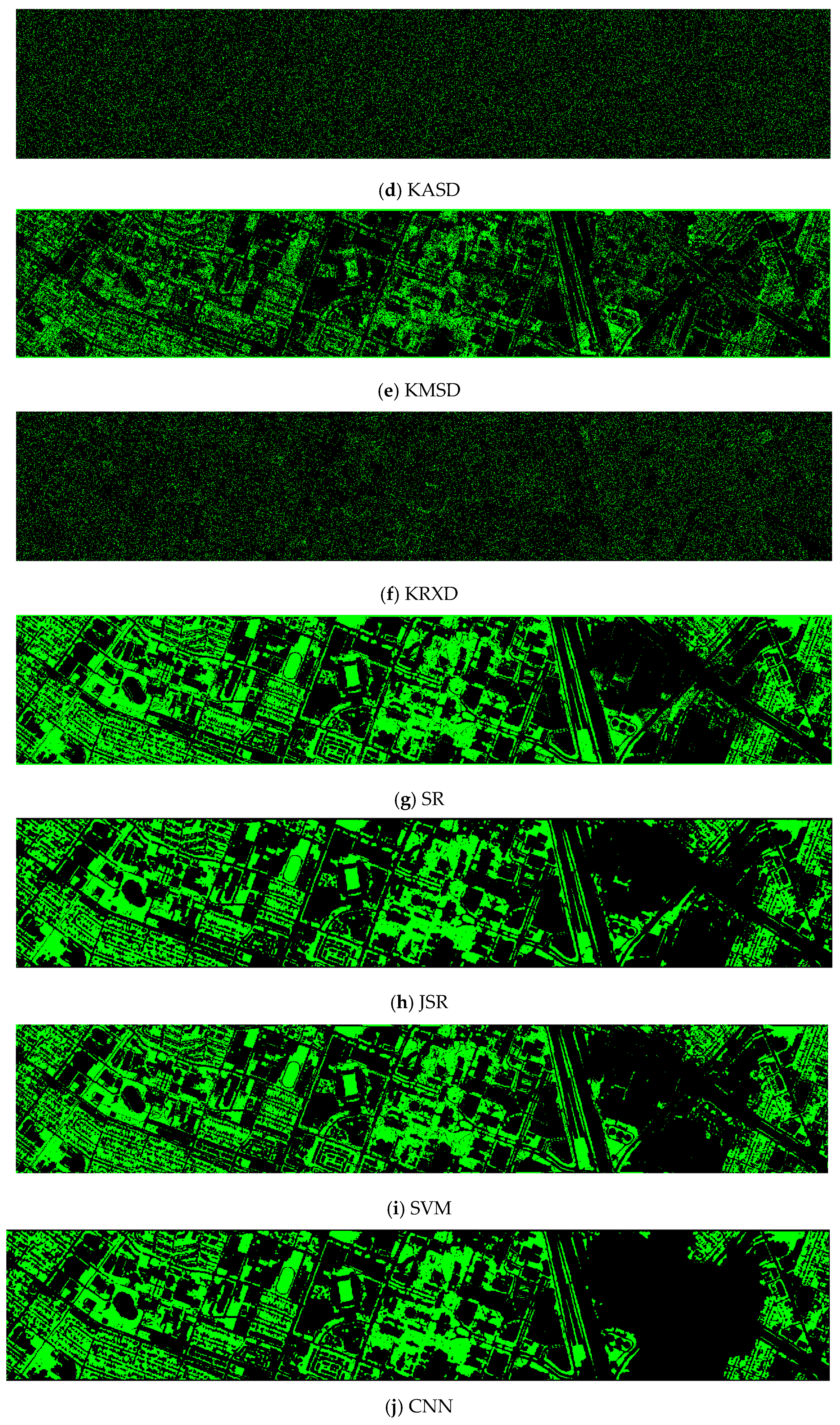
- Vegetation detection maps of nine methods for the RGB+NIR+LiDAR (DS-5) dataset
The ASD, MSD, KASD, and KRXD maps do not look good. The SR, JSR, SVM, and CNN maps look reasonable.
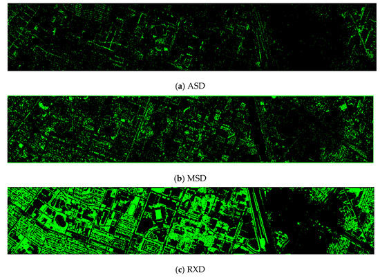
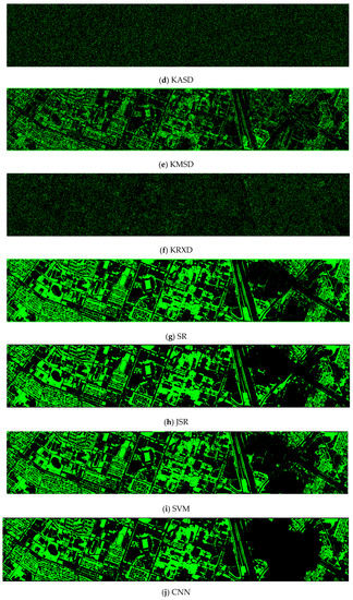
Figure A1.
Vegetation detection maps of nine algorithms for the RGB + NIR + LiDAR (DS-5) dataset. (a) ASD; (b) MSD; (c) RXD; (d) KASD; (e) KMSD; (f) KRXD; (g) SR; (h) JSR; (i) SVM; (j) CNN.
Figure A1.
Vegetation detection maps of nine algorithms for the RGB + NIR + LiDAR (DS-5) dataset. (a) ASD; (b) MSD; (c) RXD; (d) KASD; (e) KMSD; (f) KRXD; (g) SR; (h) JSR; (i) SVM; (j) CNN.
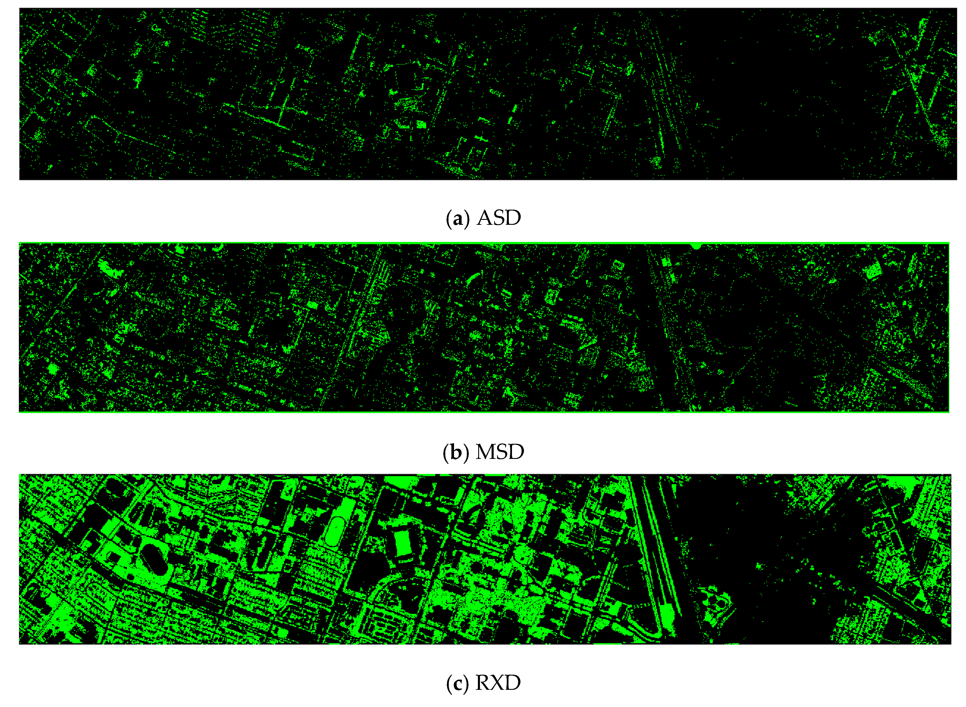
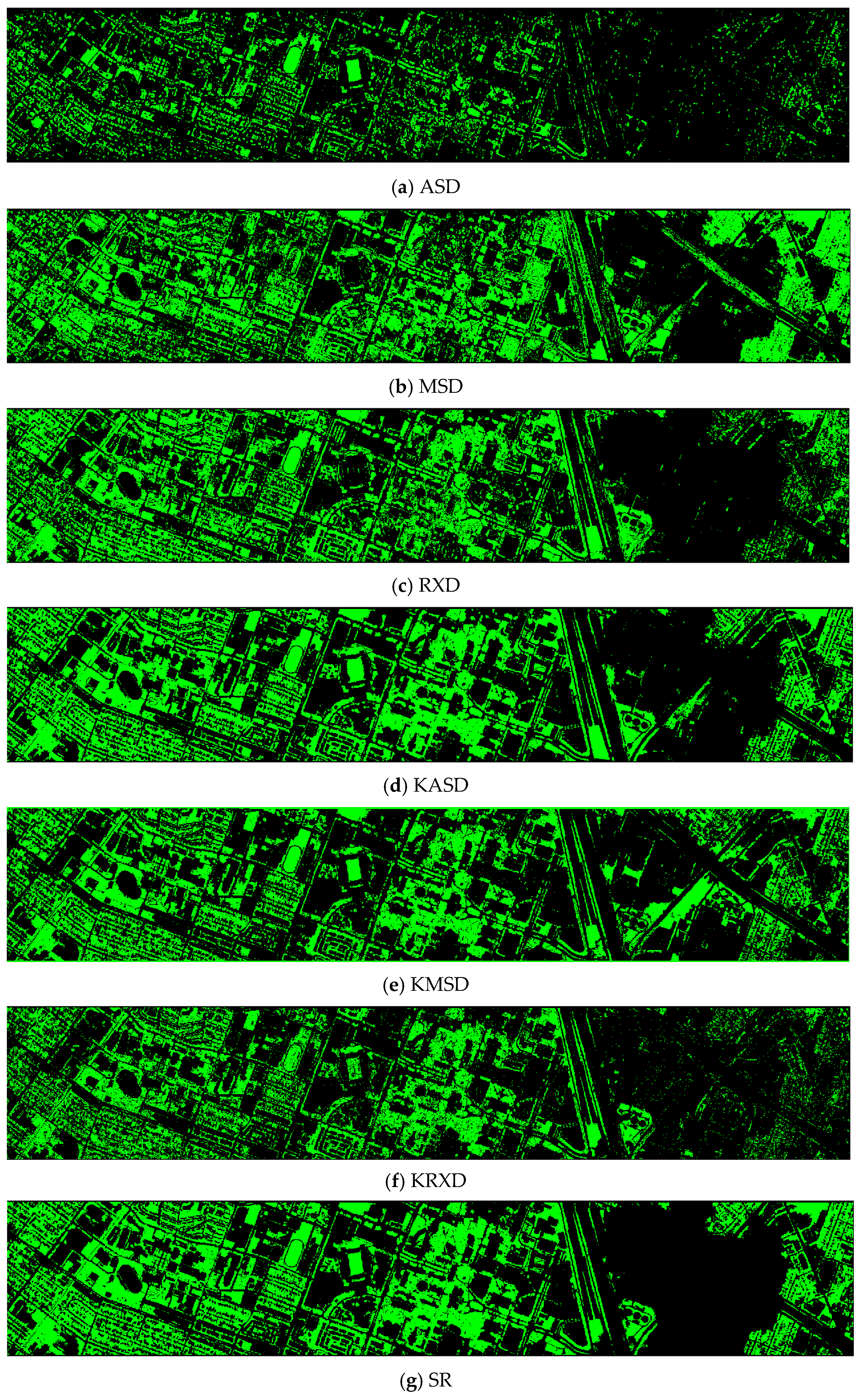
- Vegetation detection maps of nine methods for the EMAP enhanced dataset (DS-44)
Visually speaking, only ASD and KRXD maps do not look good. All others look reasonable.
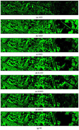
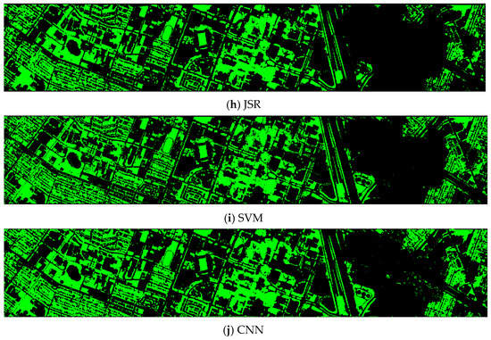
Figure A2.
Vegetation detection maps of nine algorithms for the RGB + NIR + EMAP (DS-44) dataset. (a) ASD; (b) MSD; (c) RXD; (d) KASD; (e) KMSD; (f) KRXD; (g) SR; (h) JSR; (i) SVM; (j) CNN.
Figure A2.
Vegetation detection maps of nine algorithms for the RGB + NIR + EMAP (DS-44) dataset. (a) ASD; (b) MSD; (c) RXD; (d) KASD; (e) KMSD; (f) KRXD; (g) SR; (h) JSR; (i) SVM; (j) CNN.
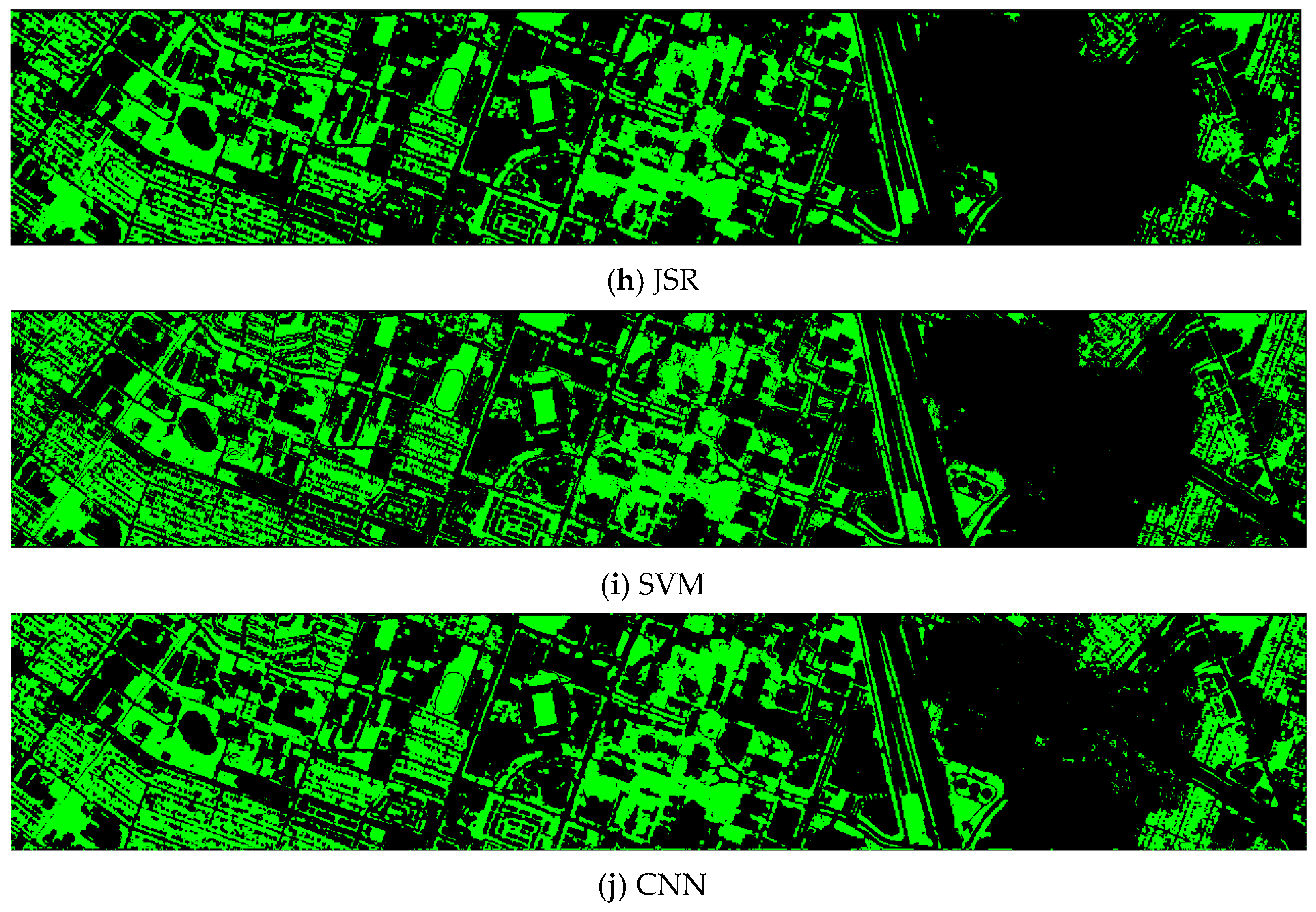
- Vegetation detection maps of nine methods for the EMAP enhanced dataset (DS-55)
RXD and KRXD maps do not look good. Others appear fine.
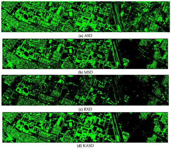
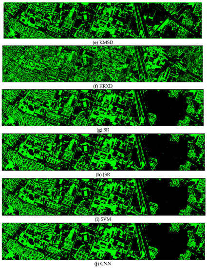
Figure A3.
Vegetation detection maps of nine algorithms for the RGB + NIR + LiDAR +EMAP (DS-55) dataset. (a) ASD; (b) MSD; (c) RXD; (d) KASD; (e) KMSD; (f) KRXD; (g) SR; (h) JSR; (i) SVM; (j) CNN.
Figure A3.
Vegetation detection maps of nine algorithms for the RGB + NIR + LiDAR +EMAP (DS-55) dataset. (a) ASD; (b) MSD; (c) RXD; (d) KASD; (e) KMSD; (f) KRXD; (g) SR; (h) JSR; (i) SVM; (j) CNN.
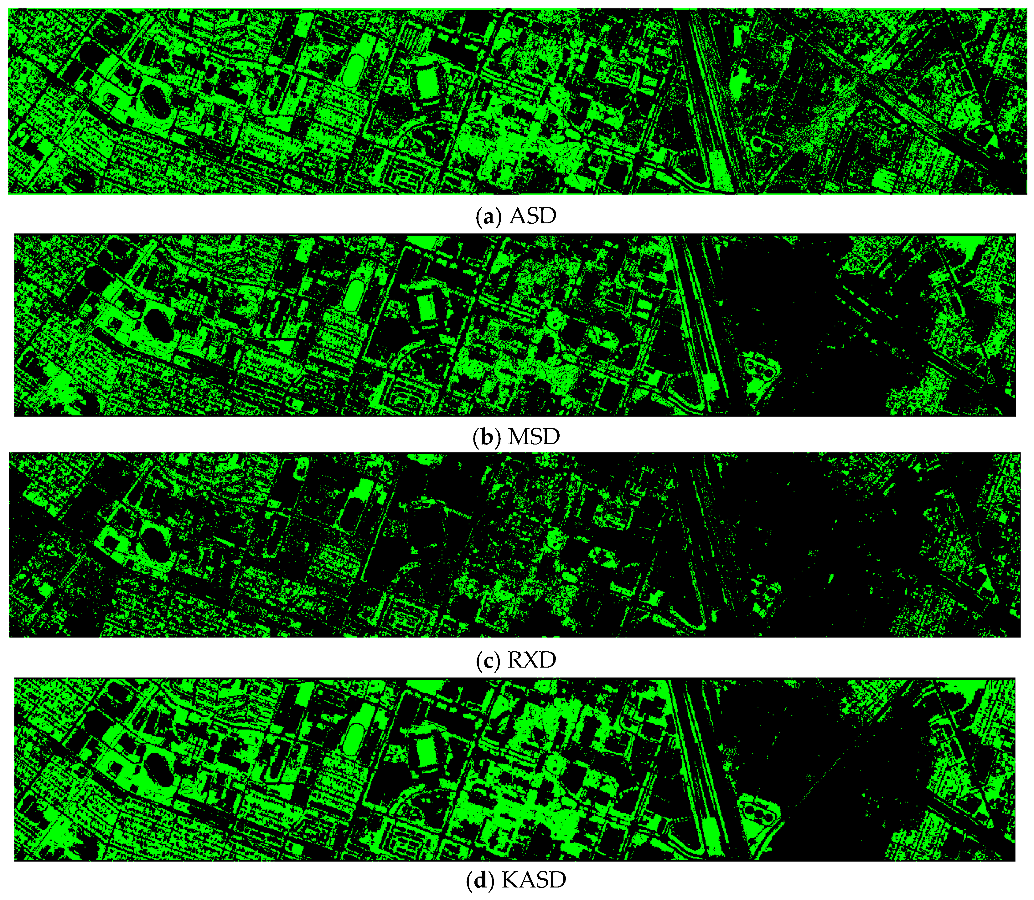
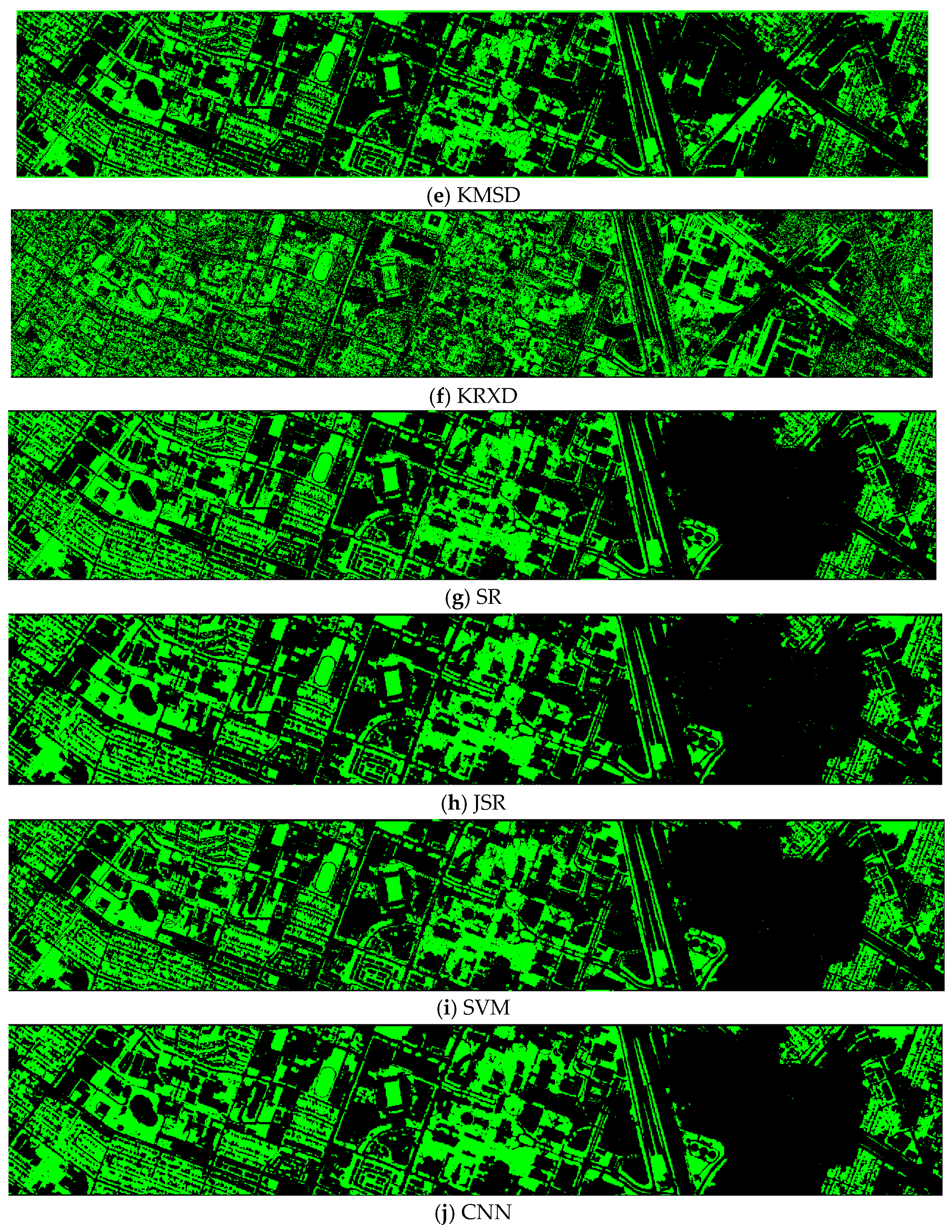
- Vegetation detection maps of nine methods for the HS dataset (DS-144)
RXD and KMSD maps do not look good. Others look just fine.

Figure A4.
Vegetation detection maps of nine algorithms for the HS (DS-144) dataset. (a) ASD; (b) MSD; (c) RXD; (d) KASD; (e) KMSD; (f) KRXD; (g) SR; (h) JSR; (i) SVM; (j) CNN.
Figure A4.
Vegetation detection maps of nine algorithms for the HS (DS-144) dataset. (a) ASD; (b) MSD; (c) RXD; (d) KASD; (e) KMSD; (f) KRXD; (g) SR; (h) JSR; (i) SVM; (j) CNN.

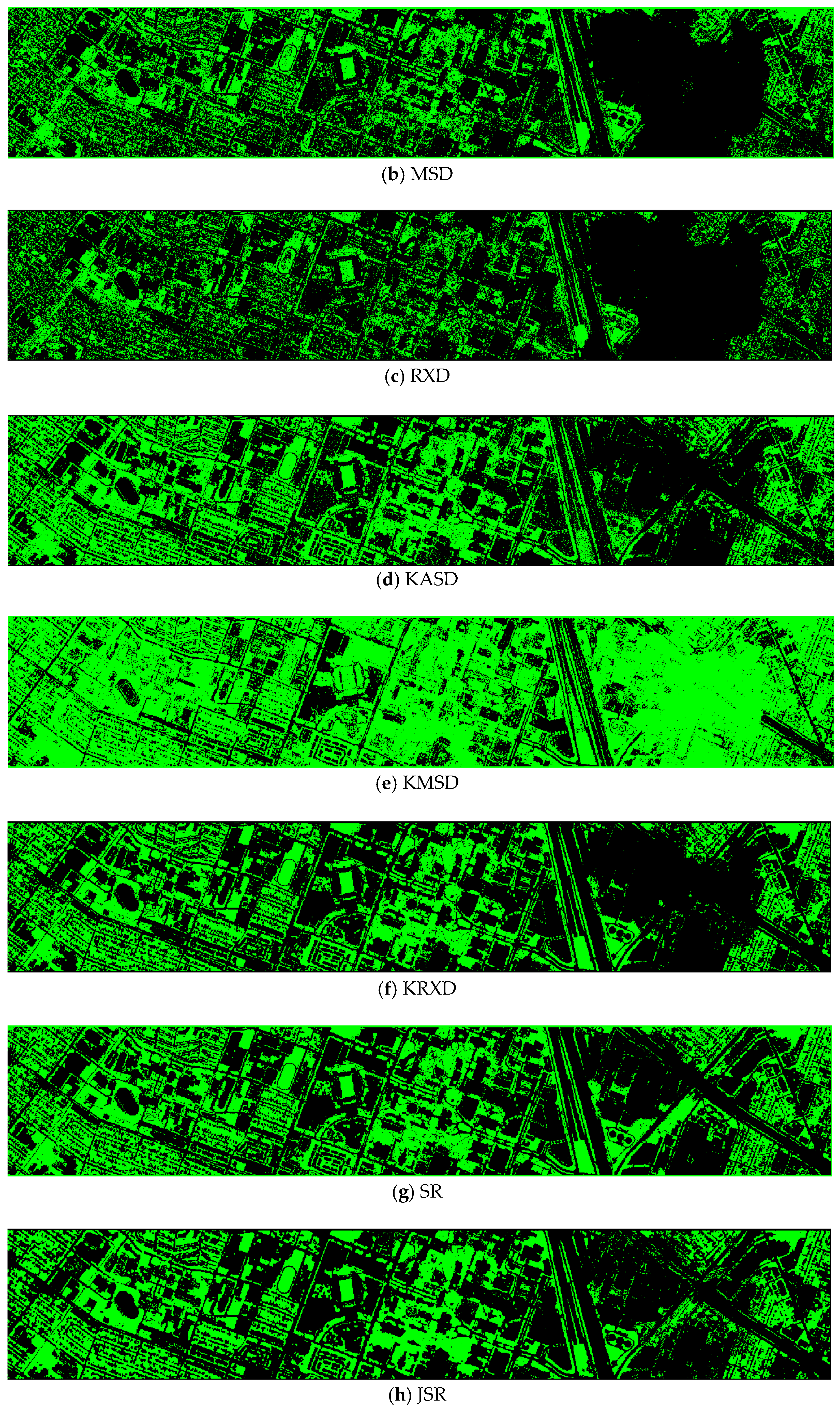
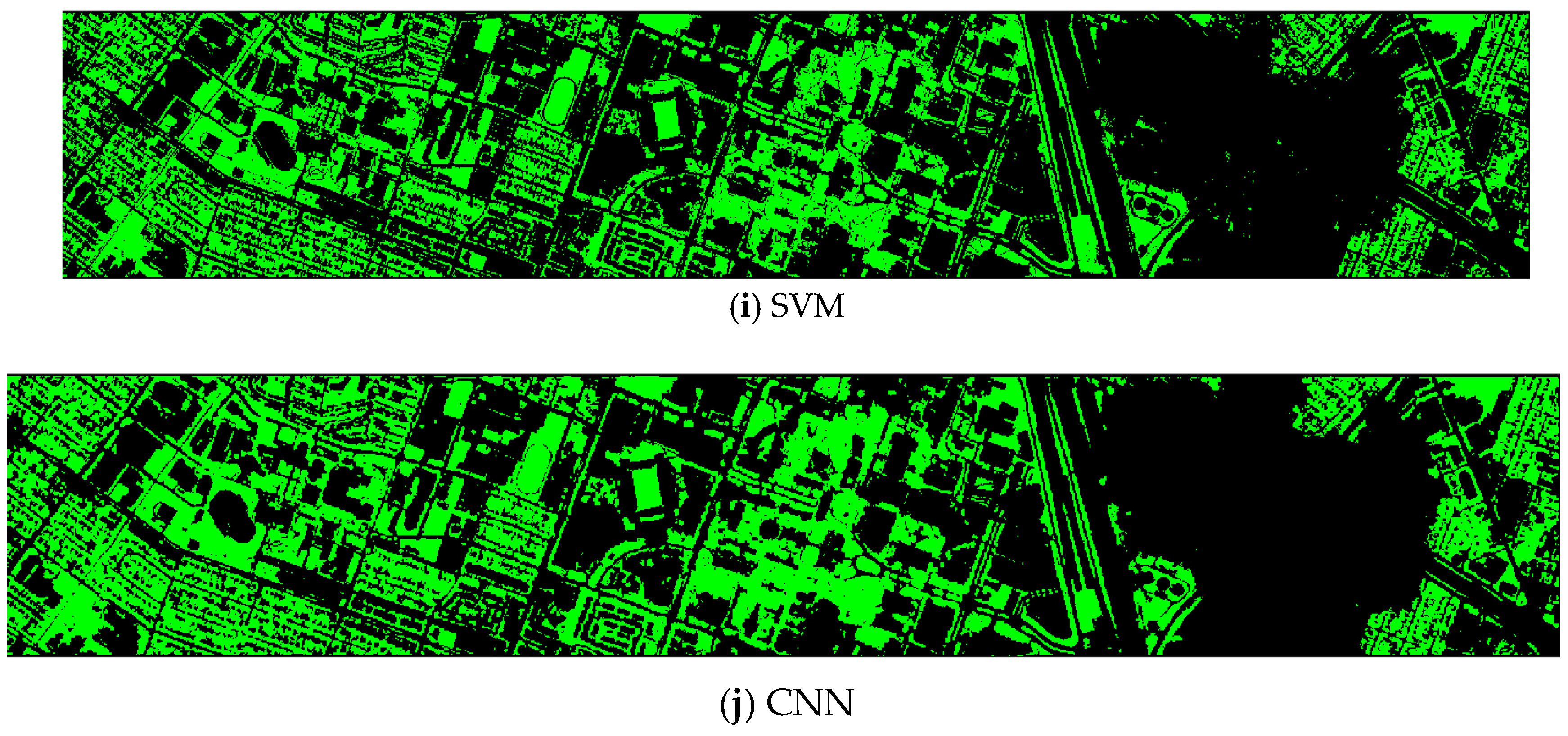
- Vegetation detection maps of nine methods for the HS dataset + LiDAR (DS-145)
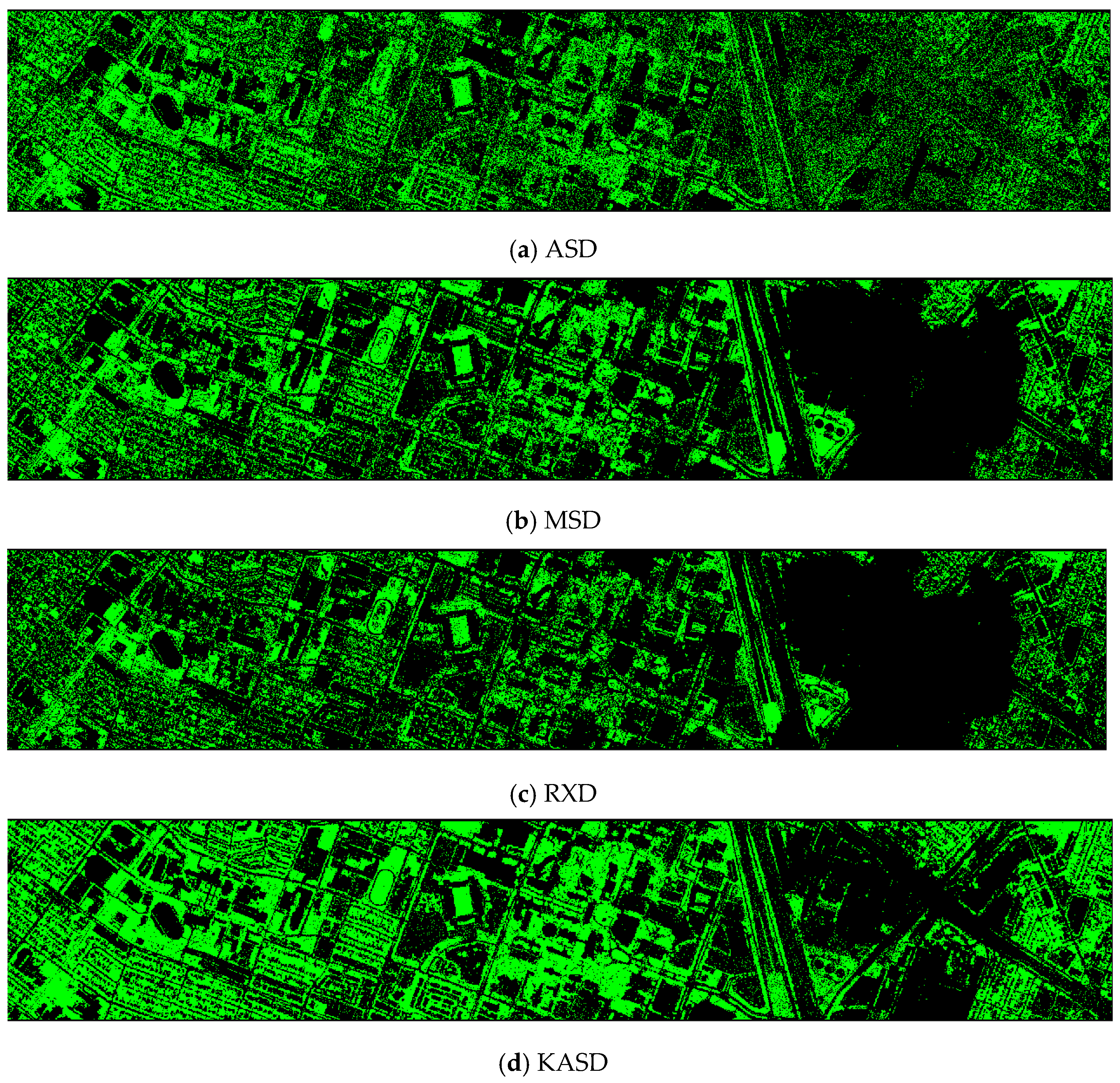
ASD, RXD, and KMSD maps do not look good. Others look fine.
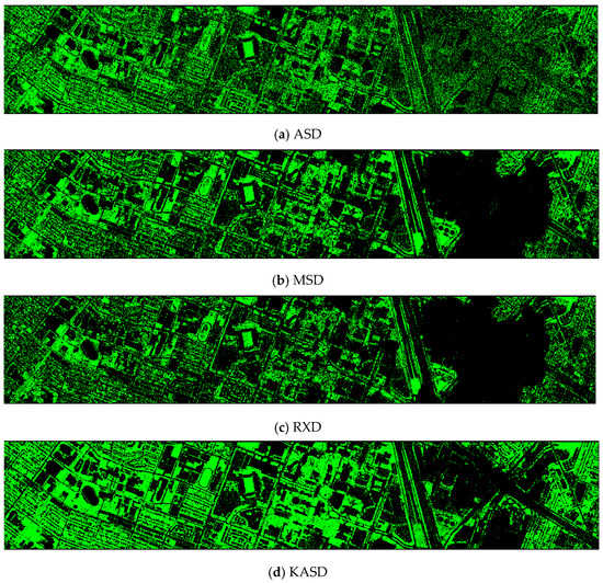
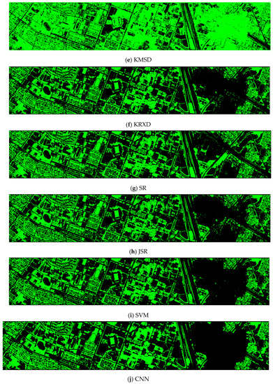
Figure A5.
Vegetation detection maps of nine algorithms for the HS + LiDAR (DS-145) dataset. (a) ASD; (b) MSD; (c) RXD; (d) KASD; (e) KMSD; (f) KRXD; (g) SR; (h) JSR; (i) SVM; (j) CNN.
Figure A5.
Vegetation detection maps of nine algorithms for the HS + LiDAR (DS-145) dataset. (a) ASD; (b) MSD; (c) RXD; (d) KASD; (e) KMSD; (f) KRXD; (g) SR; (h) JSR; (i) SVM; (j) CNN.
References
- Measuring Vegetation. Available online: https://earthobservatory.nasa.gov/features/MeasuringVegetation/measuring_vegetation_2.php (accessed on 27 May 2020).
- Yengoh, G.T.; Dent, D.; Olsson, L.; Tengberg, A.E.; Tucker, C.J., III. Use of the Normalized Difference Vegetation Index (NDVI) to Assess Land Degradation at Multiple Scales: Current Status, Future Trends, and Practical Considerations; Springer International Publishing AG: Berlin/Heidelberg, Germany, 2015. [Google Scholar]
- Bajocco, S.; De Angelis, A.; Perini, L.; Ferrara, A.; Salvati, L. The Impact of Land Use/Land Cover Changes on Land Degradation Dynamics: A Mediterranean Case Study. Environ. Manag. 2012, 49, 980–989. [Google Scholar] [CrossRef]
- Anyamba, A.; Tucker, C.J. Historical Perspectives on AVHRR NDVI and Vegetation Drought Monitoring. NASA Publ. 2012, 23, 20. [Google Scholar]
- Herrmann, S.M.; Sop, T. The map is not the territory. How satellite remote sensing and ground evidence have (Re-)Shaped the image of Sahelian desertification. In Desertification: Science, Politics and Public Perception; Behnke, R., Mortimore, M., Eds.; Earth System Science Series; Springer: New York, NY, USA, 2015. [Google Scholar]
- Mulianga, B.; Bégué, A.; Simoes, M.; Clouvel, P.; Todoroff, P. Estimating potential soil erosion for environmental services in a sugarcane growing area using multisource remote sensing data. In Remote Sensing for Agriculture, Ecosystems, and Hydrology XV; SPIE Remote Sensing: Dresden, Germany, 2013. [Google Scholar]
- De Angelis, A.; Bajocco, S.; Ricotta, C. Modelling the phenological niche of large fires with remotely sensed NDVI profiles. Ecol. Model. 2012, 228, 106–111. [Google Scholar] [CrossRef]
- Pettorelli, N.; Safi, K.; Turner, W. Satellite remote sensing, biodiversity research and conservation of the future. Phil. Trans. R. Soc. 2014, B36920130190. [Google Scholar] [CrossRef]
- Pan, C.; Zhao, H.; Zhao, X.; Han, H.; Wang, Y.; Li, J. Biophysical properties as determinants for soil organic carbon and total nitrogen in grassland salinization. PLoS ONE 2013, 8, e54827. [Google Scholar] [CrossRef]
- Liu, H.Q.; Huete, A.R. A feedback based modification of the NDVI to minimize canopy background and atmospheric noise. IEEE Trans. Geosci. Remote Sens. 1995, 33, 457–465. [Google Scholar] [CrossRef]
- Matsushita, B.; Yang, W.; Chen, J.; Onda, Y.; Qiu, G. Sensitivity of the Enhanced Vegetation Index (EVI) and Normalized Difference Vegetation Index (NDVI) to Topographic Effects: A Case Study in High-density Cypress Forest. Sensors 2007, 7, 2636–2651. [Google Scholar] [CrossRef]
- Kwan, C.; Ayhan, B.; Larkin, J.; Kwan, L.M.; Bernabé, S.; Plaza, A. Performance of Change Detection Algorithms Using Heterogeneous Images and Extended Multi-attribute Profiles (EMAPs). Remote Sens. 2019, 11, 2377. [Google Scholar] [CrossRef]
- Kwan, C.; Larkin, J.; Ayhan, B.; Kwan, L.M.; Skarlatos, D.; Vlachos, M. Performance Comparison of Different Inpainting Algorithms for Accurate DTM Generation. In Proceedings of the Geospatial Informatics X (Conference SI113), Anaheim, CA, USA, 21 April 2020. [Google Scholar]
- Ayhan, B.; Kwan, C.; Kwan, L.M.; Skarlatos, D.; Vlachos, M. Deep learning models for accurate vegetation classification using RGB image only. In Proceedings of the Geospatial Informatics X (Conference SI113), Anaheim, CA, USA, 21 April 2020. [Google Scholar]
- Ayhan, B.; Kwan, C. Tree, Shrub, and Grass Classification Using Only RGB Images. Remote Sens. 2020, 12, 1333. [Google Scholar] [CrossRef]
- Ayhan, B.; Kwan, C. Application of deep belief network to land cover classification using hyperspectral images. In Proceedings of the International Symposium on Neural Networks, Sapporo, Japan, 21 June 2017; Springer: Cham, Switzerland; pp. 269–276. [Google Scholar]
- Kwan, C.; Gribben, D.; Ayhan, B.; Bernabe, S.; Plaza, A.; Selva, M. Improving Land Cover Classification Using Extended Multi-attribute Profiles (EMAP) Enhanced Color, Near Infrared, and LiDAR Data. Remote Sens. 2020, 12, 1392. [Google Scholar] [CrossRef]
- Kwan, C.; Larkin, J.; Ayhan, B.; Budavari, B. Practical Digital Terrain Model Extraction Using Image Inpainting Techniques. In Recent Advances in Image Restoration with Application to Real World Problems; InTech: München, Germany, 2020. [Google Scholar]
- Kwan, C.; Ayhan, B.; Budavari, B.; Lu, Y.; Perez, D.; Li, J.; Bernabe, S.; Plaza, A. Deep learning for Land Cover Classification using only a few bands. Remote Sens. 2020, 12, 2000. [Google Scholar] [CrossRef]
- Bernabé, S.; Marpu, P.R.; Plaza, A.; Mura, M.D.; Benediktsson, J.A. Spectral–spatial classification of multispectral images using kernel feature space representation. IEEE Geosci. Remote Sens. Lett. 2014, 11, 288–292. [Google Scholar] [CrossRef]
- Bernabé, S.; Marpu, P.R.; Plaza, A.; Benediktsson, J.A. Spectral unmixing of multispectral satellite images with dimensionality expansion using morphological profiles. In Proceedings of the SPIE Satellite Data Compression, Communications, and Processing VIII, San Diego, CA, USA, 19 October 2012; Volume 8514, p. 85140Z. [Google Scholar]
- Mura, M.D.; Benediktsson, J.A.; Waske, B.; Bruzzone, L. Morphological attribute profiles for the analysis of very high resolution images. IEEE Trans. Geosci. Remote Sens. 2010, 48, 3747–3762. [Google Scholar] [CrossRef]
- Mura, M.D.; Benediktsson, J.A.; Waske, B.; Bruzzone, L. Extended profiles with morphological attribute filters for the analysis of hyperspectral data. Int. J. Remote Sens. 2010, 31, 5975–5991. [Google Scholar] [CrossRef]
- Skarlatos, D.; Vlachos, M. Vegetation removal from UAV derived DSMS using combination of RGB and NIR imagery. In Proceedings of the ISPRS Annals of the Photogrammetry, Remote Sensing and Spatial Information Sciences, Riva del Garda, Italy, 4–7 June 2018; Volume IV-2. [Google Scholar]
- Khodadadzadeh, M.; Li, J.; Prasad, S.; Plaza, A. Fusion of Hyperspectral and LiDAR Remote Sensing Data Using Multiple Feature Learning. IEEE J. Sel. Top. Appl. Earth Obs. Remote Sens. 2015, 8, 2971–2983. [Google Scholar] [CrossRef]
- Nasrabadi, N.M. Kernel-based spectral matched signal detectors for hyperspectral target detection. In Proceedings of the International Conference on Pattern Recognition and Machine Intelligence, Kolkata, India, 18–22 December 2007; Springer: Berlin/Heidelberg, Germany. [Google Scholar]
- Nguyen, D.; Kwan, C.; Ayhan, B. A Comparative Study of Several Supervised Target Detection Algorithms for Hyperspectral Images. In Proceedings of the IEEE Ubiquitous Computing, Electronics & Mobile Communication Conference, New York, NY, USA, 19–21 October 2017; pp. 192–196. [Google Scholar]
- Kwon, H.; Nasrabadi, N.M. Kernel RX-algorithm: A nonlinear anomaly detector for hyperspectral imagery. IEEE Trans. Geosci. Remote Sens. 2005, 43, 388–397. [Google Scholar] [CrossRef]
- Zhou, J.; Kwan, C.; Ayhan, B.; Eismann, M. A Novel Cluster Kernel RX Algorithm for Anomaly and Change Detection Using Hyperspectral Images. IEEE Trans. Geosci. Remote Sens. 2016, 54, 6497–6504. [Google Scholar] [CrossRef]
- Dao, M.; Kwan, C.; Koperski, K.; Marchisio, G. A Joint Sparsity Approach to Tunnel Activity Monitoring Using High Resolution Satellite Images. In Proceedings of the IEEE Ubiquitous Computing, Electronics & Mobile Communication Conference, New York, NY, USA, 19–21 October 2017; pp. 322–328. [Google Scholar]
- Qian, T.; Li, X.; Ayhan, B.; Xu, R.; Kwan, C.; Griffin, T. Application of support vector machines to vapor detection and classification for environmental monitoring of spacecraft. In Advances in Neural Networks—ISNN 2006, Proceedings of the Third International Symposium on Neural Networks, Chengdu, China, 28 May–1 June 2006; Springer: New York, NY, USA, 2006. [Google Scholar]
- Zhu, X.X.; Tuia, D.; Mou, L.; Xia, G.-S.; Zhang, L.; Xu, F.; Fraundorfer, F. Deep Learning in Remote Sensing: A Comprehensive Review and List of Resources. IEEE Geosci. Remote Sens. Mag. 2017, 5, 8–36. [Google Scholar] [CrossRef]
- Paoletti, M.E.; Haut, J.M.; Plaza, J.; Plaza, A. Deep learning classifiers for hyperspectral imaging: A review. ISPRS J. Photogram. Remote Sens. 2019, 158, 279–317. [Google Scholar] [CrossRef]
- Zhang, C.; Pan, X.; Li, H.P.; Gardiner, A.; Sargent, I.; Hare, J.; Atkinson, P.M. A hybrid MLP-CNN classifier for very fine resolution remotely sensed image classification. ISPRS J. Photogram. Remote Sens. 2018, 140, 133–144. [Google Scholar] [CrossRef]
- Li, W.; Fu, H.; Yu, L.; Gong, P.; Feng, D.; Li, C.; Clinton, N. Stacked Autoencoder-based deep learning for remote-sensing image classification: A case study of African land-cover mapping. Int. J. Remote Sens. 2016, 37, 5632–5646. [Google Scholar] [CrossRef]
- Bernabé, S.; Sánchez, S.; Plaza, A.; López, S.; Benediktsson, J.A.; Sarmiento, R. Hyperspectral Unmixing on GPUs and Multi-Core Processors: A Comparison. IEEE J. Sel. Top. Appl. Earth Obs. Remote Sens. 2013, 6, 1386–1398. [Google Scholar]
- Perez, D.; Banerjee, D.; Kwan, C.; Dao, M.; Shen, Y.; Koperski, K.; Marchisio, G.; Li, J. Deep Learning for Effective Detection of Excavated Soil Related to Illegal Tunnel Activities. In Proceedings of the IEEE Ubiquitous Computing Electronics and Mobile Communication Conference, New York, NY, USA, 19–21 October 2017; pp. 626–632. [Google Scholar]
- Srivastava, N.; Hinton, G.; Krizhevsky, A.; Sutskever, I.; Salakhutdinov, R. Dropout: A simple way to prevent neural networks from overfitting. J. Mach. Learn. Res. 2014, 15, 1929–1958. [Google Scholar]
- Dao, M.; Kwan, C.; Bernabé, S.; Plaza, A.; Koperski, K. A Joint Sparsity Approach to Soil Detection Using Expanded Bands of WV-2 Images. IEEE Geosci. Remote Sens. Lett. 2019, 16, 1869–1873. [Google Scholar] [CrossRef]
- Liao, W.; Pižurica, A.; Bellens, R.; Gautama, S.; Philips, W. Generalized Graph-Based Fusion of Hyperspectral and LiDAR Data Using Morphological Features. IEEE Geosci. Remote Sens. Lett. 2015, 12, 552–556. [Google Scholar] [CrossRef]
- Discussion Thread about Whether NDVI Can Be Generated Using Radiance Data. Available online: https://www.researchgate.net/post/What_is_the_difference_between_Radiance_and_Reflectance_for_Vegetation_Indices (accessed on 20 November 2020).
Publisher’s Note: MDPI stays neutral with regard to jurisdictional claims in published maps and institutional affiliations. |
© 2020 by the authors. Licensee MDPI, Basel, Switzerland. This article is an open access article distributed under the terms and conditions of the Creative Commons Attribution (CC BY) license (http://creativecommons.org/licenses/by/4.0/).


