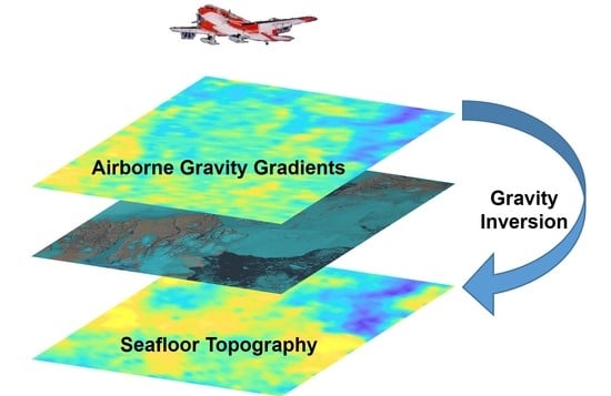
On the Feasibility of Seafloor Topography Estimation from Airborne Gravity Gradients: Performance Analysis Using Real Data

Abstract

Compared with airborne gravimetry, a technique frequently used to infer the seafloor topography at places inaccessible to ship soundings due to the presence of ice shelf or ice mélange, airborne gravity gradiometry inherently could achieve higher spatial resolution, thus it is promising for improved inference of seafloor topography. However, its estimation capability has not been demonstrated by real projects. Theoretical analysis through admittance shows that compared with gravity disturbance, gravity gradient is more sensitive to the short-wavelength seafloor topography but diminishes faster with the increase of the distance between the seafloor and airplane, indicating its superiority is recovering short-wavelength topographic features over shallow waters. We present the first numerical experiment that estimates seafloor topography from a 0.4-km resolution, real airborne gravity gradients. It is shown that airborne gravity gradiometry can recover smaller topographic features than typical airborne gravimetry, but the estimation accuracy is only $\pm 17$ m due to the presence of subsurface density variations. The long-wavelength effect of the subsurface density variations can be removed with the aid of constraining bathymetry inside the study area, whereas the short wavelengths cannot. This study expands the applications of airborne gravity gradiometry, and helps glaciologists understand its performance in seafloor topography estimation.

1. Introduction

The airborne gravimetry technique became mature in 1990s, when the appearance of GPS enabled easy access to accurate kinematic acceleration [1]. During the past three decades, airborne gravimetry has been used extensively by the glaciological communities to infer the shape of subglacial lakes [2], the seafloor topography beneath ice shelves and floating ice tongues [3,4,5,6,7,8,9], and the thickness of mountain glaciers [10], etc. At places inaccessible to ship soundings or ice-penetrating radars, airborne gravimetry has become an indispensable tool to infer seafloor topographies that are critical to study ice–ocean interactions, stability of marine-terminating glaciers, etc.

Airborne gravity gradiometry, whose line spacing is usually smaller than 0.5 km, is a more direct measure of the Earth’s gravity field at shorter wavelengths and inherently has the potential to improve not only the accuracy, but also the spatial resolution of the field for improved inference of seafloor topography. Since the late 1990s, three airborne gravity gradient survey systems, namely the airborne gravity gradiometer (AGG) by BHP Billiton Falcon, full tensor gradiometer (Air-FTG), and FTGeX by ARKeX [11], have been put into commercial operation. Measurements with these instruments enhance the natural resource exploration toolbox and have found an increasing number of applications in the past two decades [12]. However, to our knowledge, airborne gravity gradiometry has not been applied to glaciological research. Most airborne geophysical missions in polar areas, e.g., Operation IceBridge [13], Oceans Melting Greenland [14], use airborne gravimeters to measure the gravity field. A question then naturally arises: can airborne gravity gradients be used in similar missions to infer the seafloor topography for the purpose of achieving higher spatial resolution and accuracy? Both airborne gravity gradients data and high-resolution multibeam bathymetric data exist in St. George’s Bay, Newfoundland, Canada, a region on the inner continental shelf like that of several earlier projects [3,4,5,6,7,8] studying the interactions between the ocean and marine-terminating glaciers, and thus enables us to examine the performance of airborne gravity gradients in seafloor topography estimation. This paper analyzes the advantages and limitations of using the gravity gradients to estimate the seafloor topography, and for the first time provides a numerical experiment showing the results of airborne-gravity-gradient-inferred seafloor topography. This paper extends the application of airborne gravity gradiometry to seafloor topography estimation, and helps glaciologists understand the performance of the airborne gravity gradients in seafloor topography estimation.

2. Comparison between Airborne Gravimetry and Airborne Gravity Gradiometry

2.1. Resolution

The acceleration sensed by an airborne gravimeter is specific force. In the inertial frame, it is the combination of the gravitational acceleration and the kinematic acceleration of the aircraft [15]. Therefore, in addition to the airborne gravimeter, the accuracy of the measured gravity is also affected by the kinematic acceleration derived from aircraft tracking (typically using differentially corrected GPS). Limited by the errors in modeling the numerical derivative and the positioning capabilities of current global navigation satellite systems, the kinematic acceleration can achieve an accuracy of sub-mGal level only with smoothing over intervals of 60s or longer [16]. On the contrary, airborne gravity gradiometry does not need to determine the kinematic acceleration of the aircraft. As a result, the resolution of airborne gravity gradients (typically 0.5 km) is higher than the resolution of airborne gravity measured by a fixed-wing aircraft (typically 2 km). This implies that airborne gravity gradiometry is superior in detecting small topographic features, which is particularly desirable in studies at the individual glacier scale.

2.2. Admittances

Parker’s infinite series [17] is a formula to calculate the gravitational acceleration caused by a non-uniform volume of material. The regional isostatic compensation mechanism [18] treats the lithosphere as a thin elastic plate that flexes under the load (i.e., topography). Assuming that the measured gravity is only caused by the topography and the corresponding flexure of the lithospheric plate at the Mohorovicic discontinuity (the density interface between the crust and mantle) [19], we combine the first-term approximation of Parker’s series and the regional isostatic compensation mechanism to establish the relationship between gravity and topography in the spectral domain.

Assuming the density of the crust is uniform, the gravitational acceleration at sea surface, $\delta g$, caused by $b$, the deviation of the seafloor from the mean sea depth $d$, is given by (detailed derivations can be found in pp. 23–26 of [20]):

$$ℱ\left(\delta g\right)=-2\pi G\mathsf{\Delta }\rho e^{-2\pi \overline{f}d}\left[1-{\Phi }_e\left(\overline{f}\right)e^{-2\pi \overline{f}t}\right]ℱ\left(b\right),$$

(1)

where $ℱ$ denotes 2-D Fourier transform, $G$ is the gravitational constant, $\mathsf{\Delta }\rho$ is the density difference between the crust and sea water, $\overline{f}$ is the radial frequency, $t$ is the mean thickness of the crust, and ${\Phi }_e\left(\overline{f}\right)$ is the spectral domain function that modifies the Airy response so as to produce the flexure of the lithosphere [19]:

$${\Phi }_e\left(\overline{f}\right)={\left[\frac{16D{\pi }^4{\overline{f}}^4}{\left({\rho }_m-{\rho }_c\right)g}+1\right]}^{-1},$$

(2)

where $g$ is the gravitational acceleration, ${\rho }_m$ and ${\rho }_c$ are the density of the mantle and crust, respectively, and $D$ is the flexural rigidity of the plate given by:

$$D=\frac{E{T}_e^3}{12\left(1-{\upsilon }^2\right)},$$

(3)

where $E$ is Young’s modulus, $\upsilon$ is Poisson’s ratio, and $T_e$ is the elastic thickness of the plate.

The vertical-vertical gravity gradient (VGG) at sea surface, ${\Gamma }_{zz}$, caused by $b$, is given by:

$$ℱ\left({\Gamma }_{zz}\right)=4{\pi }^2\overline{f}G\mathsf{\Delta }\rho e^{-2\pi \overline{f}d}\left[1-{\Phi }_e\left(\overline{f}\right)e^{-2\pi \overline{f}t}\right]ℱ\left(b\right).$$

(4)

In Equation (1), the spectral domain parameter that modifies the seafloor topography so as to produce the gravity disturbance is called the gravitational admittance, $Z_{\delta g}\left(\overline{f}\right)$. The theoretical gravitational admittance is:

$$Z_{\delta g}\left(\overline{f}\right)=\frac{ℱ\left(\delta g\right)}{ℱ\left(b\right)}=-2\pi G\mathsf{\Delta }\rho e^{-2\pi \overline{f}d}\left[1-{\Phi }_e\left(\overline{f}\right)e^{-2\pi \overline{f}t}\right].$$

(5)

Similarly, based on Equation (4) the gravity gradient admittance $Z_{{\Gamma }_{zz}}\left(\overline{f}\right)$ is defined as:

$$Z_{{\Gamma }_{zz}}\left(\overline{f}\right)=\frac{ℱ\left({\Gamma }_{zz}\right)}{ℱ\left(b\right)}=4{\pi }^2\overline{f}G\mathsf{\Delta }\rho e^{-2\pi \overline{f}d}\left[1-{\Phi }_e\left(\overline{f}\right)e^{-2\pi \overline{f}t}\right].$$

(6)

In summary, under certain assumptions (constant density, constant-height measurement surface above all masses, linear approximation), the gravity disturbance and gravity gradients can be approximately related to the seafloor topography in the spectral domain through the admittances:

$$ℱ\left(\delta g\right)=Z_{\delta g}\left(\overline{f}\right)ℱ\left(b\right),$$

(7)

$$ℱ\left({\Gamma }_{zz}\right)=Z_{{\Gamma }_{zz}}\left(\overline{f}\right)ℱ\left(b\right).$$

(8)

Next, we use the theoretical gravitational admittance and gravity gradient admittance to analyze the advantages and limitations of using the gravity gradients to estimate the seafloor topography. The theoretical admittances (5) and (6) are computed using the values in

Table 1. Parameters used to calculate the admittances in Figure 1 and Figure 2.

Parameter	Value
${\rho }_w$, density of sea water	1030 kg/m3
${\rho }_c$, density of the crust	2670 kg/m3
${\rho }_m$, density of the mantle	3330 kg/m3
$d$, mean depth of sea water	4500 m
$t$, mean thickness of the crust	6000 m
$E$, Young’s modulus	$7\times {10}^{10}$ kg·m−1·s−2
$\upsilon$, Poisson’s ratio	0.27
$T_e$, effective elastic thickness	45,000 m

and are shown in Figure 1 and Figure 2.

The top panel of Figure 1 shows that at long wavelengths, the admittance function is sensitive to the compensation scheme (i.e., the choice of the effective elastic thickness of the plate $T_e$). As can be found by comparing the uncompensated (solid curve) and compensated (dashed curves) admittances in the top panel of Figure 1, at long wavelengths, the gravity disturbance generated by seafloor topography is partially cancelled out by isostatic compensation, which in fact is uncertain to a large extent. Besides, the density variations within the mantle, if they exist, affect the gravity disturbance at the sea surface mainly in the long wavelengths because the short-wavelength gravity disturbance is attenuated in the upward continuation [21]. In summary, the theoretical relationship between gravity disturbance and seafloor topography contains large uncertainties at long wavelengths. It is one of the reasons why predicting seafloor topography from gravity disturbances based on their theoretical relationship is feasible only at a certain short-to-intermediate, uncompensated wavelength band [22]. As a result, a long-wavelength regional gravity should be removed prior to the inversion when predicting seafloor topography from airborne gravity disturbances. In previous studies, the regional gravity is empirically computed through various methods, such as spherical harmonic models [5,23,24], upward continuation [25,26], matched filters [27], etc. However, a large discrepancy exists between the regional gravity computed by different methods, so does the corresponding gravity-disturbance-estimated seafloor topography. Along with the uniform density assumption to the bedrock, the uncertainty in the regional gravity is one of the largest error sources in gravity-based seafloor topography estimation [28].

The bottom panel of Figure 1 shows that the isostatic compensation has smaller effects on the gravity gradient admittance than on the gravitational admittance. Besides, due to the $-2\pi \overline{f}$ factor in the gravity gradient admittance, i.e., Equation (6), the VGG is less sensitive to the long-wavelength topography than the gravity disturbance. This indicates that when predicting seafloor topography from airborne gravity gradients, removing the long-wavelength regional gravity gradient is not necessary, so the uncertainties associated with the computation of regional gravity is avoided.

On the other hand, the gravity gradient admittance reaches its maximum at wavelength 75 km, whereas the peak of the gravitational admittance is at the longer wavelengths. This difference is even larger if we use a smaller mean sea depth (see Figure 2). This indicates that gravity gradient has higher relative magnitude at short wavelengths than gravity disturbance. From another perspective, compared to the gravity disturbance, the gravity gradient is more sensitive to short-wavelength topography. Because the prediction band is in the short-to-intermediate wavelengths, we may conclude that the gravity gradient is superior to the gravity disturbance in seafloor topography estimation.

One should note that the gravity gradient diminishes with the cube of distance between the mass element and the measurement point, while gravity disturbance attenuates with the square of distance. So, for deep ocean areas, the magnitude of the gravity gradient at the sea surface may be small, which then also implies a small signal-to-noise ratio. For these areas, the superiority of the gravity gradient at short wavelengths may be cancelled by the low signal-to-noise ratio because the attenuation rate of gravity disturbance is slower. The variation of admittance with respect to mean sea depth is shown in Figure 2. As the mean sea depth increases, the gravity gradient admittance decreases fast, and the peak of the admittance gradually moves to longer wavelengths. Although the gravitational admittance also decreases when mean sea depth increases, the change rate is comparatively slower.

3. Numerical Experiments

As analyzed in Section 2, compared with airborne gravity disturbance, airborne gravity gradient avoids uncertainties associated with the regional gravity, is more sensitive to the short-wavelength seafloor topography, and thus is considered superior when predicting seafloor topography over shallow waters. This section uses high-resolution (0.4 km) airborne gravity gradient data in a small region (12.6 km × 18.4 km) to infer the seafloor topography, for the purpose of investigating its ability to detect small topographic features in offshore areas.

3.1. Airborne Gravity Gradients and Multibeam Bathymetry

In December 2012, Bell Geospace Inc. (BGI), Houston, TX, USA conducted a gravity gradiometry survey over St. George’s Bay [29]; see Figure 3a. It is located off the southwestern shore of Newfoundland, Canada. The FTG full tensor gradiometer is installed on a Basler Turbo BT-67 aircraft, which was flown to gently drape the land topography in order to minimize the distance between measurement altitude and ground. The reported accuracy of the FTG is about 5 to 7 Eötvös [29]. The designed (nominal) flight altitude during the entire survey is 80 m above the water. The flight lines are 400 m apart, with data sampled along-track at a one second interval, which translates to a 59.7-m spatial sampling interval using the 215 km/h speed. As part of the data processing, BGI projected the gravity gradients onto the Universal Transverse Mercator (UTM) zone 21 N.

High horizontal resolution (10 m × 10 m) multibeam bathymetry data for this area were obtained from the Geological Survey of Canada (Atlantic) [30]; see Figure 3b. The reported accuracy of the multibeam echo sounding is usually in the level of 10 cm [31]. Besides, the accuracy of the multibeam sounding is generally evaluated according to the International Hydrographic Organization Standards for Hydrographic Surveys [32], which requires the uncertainty of the reduced depths to be smaller than $0.25+0.0075\times b$ meter, where b is the seafloor depth (the mean depth of the study area is 38.56 m). It is much smaller than the accuracy of the gravity estimated seafloor topography. Therefore, the bathymetric data are treated as true depths to evaluate the accuracy of the gravity-gradient-inferred seafloor topography.

3.2. Inversion Methods

The seafloor topography is estimated from airborne gravity gradients using very fast simulated annealing (SA) [33], a global optimization method that can process high-dimensional nonlinear inversion problems. The SA algorithm iteratively searches over a set of candidate seafloor topographies. During each iteration, the gravity gradients are forward computed from seafloor topography and compared with the measured gravity gradients. The SA algorithm can asymptotically find an optimal seafloor topography that minimizes the discrepancy between the measured and forward-computed gravity gradients. Interested readers are referred to [8,34] for a more detailed description of the SA method. In the remainder of this subsection, we only describe the key steps of SA, namely the forward model and the cost function (defined in the next paragraph).

We discretize the study region (inside the dashed lines shown in Figure 3b) into adjacent right rectangular prisms with a horizontal dimension of 400 m × 400 m. Each prism is assigned a uniform density representing either sea water (1030 kg/m³) or bedrock (2200 kg/m³ [29]). The gravity gradient at flight altitude, treated as the effect of mass deficiency caused by the sea water between the sea surface and the seafloor, is forward computed from the right rectangular prisms model using Nagy et al.’s formula [35]. For each computation point, only the prisms within 23 km of horizontal distance from the point are used in the forward computation. According to formulas given by Jekeli [36], the errors introduced by neglecting the masses outside the 23-km inner zone is 0.5 Eötvös, which is one order smaller than the accuracy of the gravity gradient measurements. Note that the seafloor topography model was extended by 23 km from each of the four sides of the study region to enable the forward computation at the study region margin. The resolution of the extended seafloor topography is still 400 m by 400 m. The extended seafloor topography in regions not covered by multibeam bathymetry is interpolated from the global topography model version 18.1 released by the Scripps Institution of Oceanography [22], whose spatial resolution is about 1230 m. The cost function is an indicator that measures the discrepancy between the forward computed and measured gravity gradients. In this study, it is defined as the $L^2$ norm of the difference between the forward computed and measured gravity gradients.

3.3. Analysis and Removal of the Non-Terrain Effects

The high-resolution high-accuracy multibeam bathymetric data shown in Figure 3b enable us to analyze the gravity gradients caused by non-terrain factors (called the non-terrain effects). Firstly, the gravity gradients at flight altitude were forward computed from the multibeam bathymetry represented by adjacent right rectangular prisms. They are called the terrain effects and are shown in Figure 4a. Note that for each computation point, only prisms within its inner zone of radius, 23 km, were used in the forward computation. The gravity gradient due to one prism was computed using formulas in [35]:

$${\Gamma }_{zz}={{{G\rho \arctan \frac{\left(x-\xi \right)\left(y-\eta \right)}{\left(z-\zeta \right)\sqrt{{\left(x-\xi \right)}^2+{\left(y-\eta \right)}^2+{\left(z-\zeta \right)}^2}}|}_{\xi =x_1}^{x_2}|}_{\eta =y_1}^{y_2}|}_{\zeta =z_1}^{z_2},$$

(9)

where $\rho$ is the density of the right rectangular prism, $\left(x, y, z\right)$ are the coordinates of the computation point, $\left(\xi , \eta , \zeta \right)$ are the variables of integration over the right rectangular prism, $\left[x_1, x_2\right], \left[y_1, y_2\right]$ and $\left[z_1,z_2\right]$ are the $x$ axis, $y$ axis, and $z$ axis boundaries of the right rectangular prism, respectively. Next, the difference between the measured gravity gradients and the terrain effects is defined as the non-terrain effects and shown in Figure 4b. The non-terrain effects are caused by the sub-topography density anomalies, regional isostatic compensation, and model errors in the forward computation due to the neglected masses outside the 23-km inner zone. Since the model errors are in the level of 0.5 Eötvös [36], and the isostatic compensation is a regional effect that is not significant over small regions [18], the non-terrain effects shown in Figure 4b are mainly attributed to the sub-topography density anomalies.

Comparison between Figure 4a and Figure 3a shows that the terrain effect contributes less than 50% of the gravity gradient measurements (the RMS of the terrain effect shown in Figure 4a is about 49.13% of the RMS of the directly measured gravity gradients shown in the black dashed rectangle in Figure 3a). Topography estimation from gravity gradients in this area is feasible yet inaccurate since sub-topography density variation introduces large errors. So, the non-terrain effects shown in Figure 4b should be removed prior to the inversion. Recent studies [4,7,8,37,38] tend to remove the non-terrain effects by (1) calculating the difference between the measured and forward-computed VGGs over areas constrained by bathymetric data or land surface elevation, (2) interpolating this difference into areas without constraining data using a minimum curvature algorithm [39], (3) and then subtracting the interpolated difference from the measured VGGs. This method is practical in offshore areas, where land surface elevation (e.g., from the GIMP model [40]) or sparse ship soundings are usually available inside or in the surrounding of the study area to provide the constraints [3,4,5,6,7,8]. We examined the performance of this method by designing 5 experiments with different constraints. Experiment No. 1 directly estimates the seafloor topography from the measured VGGs without removal of the non-terrain effects. Experiment No. 2 assumes that the bathymetric depths in the surrounding of the study area (see Figure 5a) are available to the researchers, estimates the non-terrain effects (see Figure 5d) using constraints from known bathymetry, and removes them from the measured VGGs prior to the inversion. Experiment No. 3 assumes that sparse ship soundings inside the study area (see Figure 5b) are also available to the researchers. Experiment No. 4 increases the amount of available ship soundings inside the study area (see Figure 5c). Besides, we also added experiment No. 0 to examine the reliability of the simulated annealing method. Experiment No. 0 estimates seafloor topography from the synthesized VGGs shown in Figure 4a that are forward computed from multibeam bathymetric data. This means the non-terrain effects were completely removed, so ideally the estimated seafloor topography should be consistent with the multibeam bathymetry.

Comparison between the actual non-terrain effects (shown in Figure 4b) and the estimated non-terrain effects (shown in Figure 5d–f) indicates that experiment No. 2 to No. 4 only removes the long-wavelength component of the non-terrain effects from the measured VGGs. The difference between them is the residual error in the input to the inversion model estimating the seafloor topography, and is shown in

Table 2. Statistics of the residual error, namely the difference between the actual non-terrain effects shown in Figure 4b and the estimated non-terrain effects removed in experiment No. 0 to No. 4.

No.	Mean	STD	RMS
0	0	0	0
1	16.77	14.25	22.01
2	−0.11	14.52	14.52
3	−1.09	11.36	11.41
4	−0.23	10.39	10.39

Note. The units are Eötvös. STD = standard deviation; RMS = root mean square.

. Experiment No. 1 directly uses the measured VGGs, so its residual error is the actual non-terrain effects. Experiment No. 0 uses the terrain effect as input to the inversion model. This is equivalent to a complete removal of the non-terrain effects, so its residual error is 0.

3.4. Results, Evaluation, and Discussion

The SA programs of the five experiments were run on the supercomputer Oakley at the Ohio Supercomputer Center. Each program exited after $1\times {10}^7$ iterations. The estimated seafloor topographies are shown in Figure 6. The multibeam bathymetry is treated as the true depth to evaluate the accuracy of the seafloor topography estimated from airborne gravity gradients using SA. The statistics of the difference between them are shown in

Table 3. (a) Statistics of the difference between the multibeam bathymetry and the seafloor topography estimated from gravity gradients using simulated annealing; (b) Statistics of the difference between the measured gravity gradients and the one forward computed from the seafloor topography estimation.

	(a) 1			(b) 2
No.	Mean	STD	RMS	Mean	STD	RMS
0	1.56	2.64	3.06	0.11	0.29	0.31
1	14.39	19.27	24.05	−0.08	6.23	6.23
2	9.39	22.43	24.32	0.75	5.75	5.80
3	9.00	14.82	17.34	1.12	4.20	4.35
4	11.60	14.05	18.22	0.87	4.29	4.37

¹ The units are meters. ² The units are Eötvös.

. The statistics of the difference between the measured VGGs and the one forward computed from the seafloor topography estimation are shown in Table 3 too.

Figure 6a shows that the seafloor topography was successfully recovered from the synthesized VGGs shown in Figure 4a using SA, with estimation error of $\pm 3$ m. The error is mainly caused by the large dimensionality of the inversion, and the comparatively small number of iterations used. This confirms the reliability of simulated annealing in recovering the seafloor topography, so that the estimation error in the other four experiments is mainly attributed to the sub-seafloor density variations.

Figure 6b shows that experiment No. 1 recovers the general shape of the seafloor topography, including the sharp drop at 375 km Easting, the 2-km-wide Y-shaped trough system at the southeast corner and its 0.8 km wide branch at km [378.5, 5365]. Considering the typical resolution of airborne gravimetry is 2 km (capable of recovering topographic features with wavelength longer than 4 km), it is shown that the airborne gravity gradient is capable of recovering shorter-wavelength topographic features than gravity disturbance. However, the estimation error is as large as $\pm 24$ m. This is because the airborne gravity gradient measurements used in this study were conducted for geologic purposes in areas with complex sub-topography geologic structures, where the assumption of uniform density does not hold. The large non-terrain effects (22 Eötvös RMS, mainly due to sub-seafloor density variations) prevents experiment No. 1 from achieving high estimation accuracy. This experiment highlights the need to remove the non-terrain effects. Note that this is not the drawback of the airborne gravity gradiometry. In seafloor topography estimations using gravity disturbance, the non-terrain effect is one of the largest error sources too [22,28].

Experiments No. 2 to No. 4 remove the non-terrain effects using constraints from known bathymetry. In experiment No. 2, the non-terrain effects are estimated from constraining bathymetry in the surrounding of the study area. Figure 6c and Table 3 indicate that compared with experiment No. 1, experiment No. 2 does not improve the estimation accuracy. This can be explained through the residual errors shown in Table 2. The STD of the residual error in experiment No. 1 is in the same level with that in experiment No. 2. Experiment No. 3 has constraining bathymetry both inside and in the surrounding of the study area. Figure 6d and Table 3 indicate that the estimation accuracy is improved to $\pm 17$ m. Experiment No. 4 increases the amount of the bathymetric data inside the study area, but surprisingly, Figure 6e and Table 3 do not show improvements in the estimation accuracy. Probably it is because the randomly selected constraining bathymetry does not capture the proper feature points of the seafloor topography. Combining these results and the comparison between Figure 4b with Figure 5d–f, it is shown that the sparse bathymetric constraints could be used to remove the long-wavelength component of the non-terrain effects, which highlights the need to make future gravity gradiometry survey overlap the known bathymetry or land surface elevations.

4. Conclusions

Airborne gravimetry has been used extensively by the glaciological community to estimate the seafloor topography at places covered by ice shelves, iceberg, or ice mélange, which are inaccessible to traditional ship soundings. Airborne gravity gradiometry is an alternative source of gravity data. It inherently has the potential to achieve higher spatial resolution for improved inference of seafloor topography, and thus is in need of demonstration. By analyzing the theoretical admittances, we demonstrated the superiority of airborne gravity gradient in recovering small topographic features over shallow waters. We also present the first numerical experiments that use real airborne gravity gradient data to estimate the seafloor topography. Understandably, we achieved only moderate success since in our study area, the unknown variations in subsurface mass density dominate the gravity gradient signal over that caused by the geometric configuration of the seafloor. It is shown that airborne gravity gradiometry can recover small topographic features that are outside of the resolution capability of typical airborne gravimetry, but the estimation accuracy is only $\pm 17$ m due to the presence of large non-terrain effects. The long-wavelength non-terrain effect can be removed if sparse bathymetric data are available inside the study area to provide constraints, whereas the short wavelengths cannot. This suggests that future airborne gravity gradiometry survey should overlap some known bathymetry or land surface elevations, and that more advanced non-terrain effect removing techniques should be investigated in the future to fully realize the potential of the airborne gravity gradients at short wavelengths. We remain optimistic about seafloor topography estimation from airborne gravity gradients, since at some places, the subsurface density variation is significant while at some other places the density of terrain is almost constant, where the non-terrain effect is small. Future studies at places where the density of terrain is almost uniform are needed to fully demonstrate the estimation capability of airborne gravity gradients. This study is an important starting point for future work that constantly improves glaciologists’ understanding of the advantage and performance of airborne gravity gradients in seafloor topography estimation. This study could help glaciologists make better decisions when selecting gravity measurement devices for future airborne geophysical missions in polar areas.

References

1. Jekeli, C. Vector gravimetry using GPS in free-fall and in an Earth-fixed frame. J. Geod. 1992, 66, 54–61. [Google Scholar] [CrossRef]
2. Studinger, M.; Bell, R.E.; Tikku, A.A. Estimating the depth and shape of subglacial Lake Vostok’s water cavity from aerogravity data. Geophys. Res. Lett. 2004, 31, 1–4. [Google Scholar] [CrossRef] [Green Version]
3. Greenbaum, J.S.; Blankenship, D.D.; Young, D.A.; Richter, T.G.; Roberts, J.L.; Aitken, A.R.A.; Legresy, B.; Schroeder, D.M.; Warner, R.C.; Van Ommen, T.D.; et al. Ocean access to a cavity beneath Totten Glacier in East Antarctica. Nat. Geosci. 2015, 8, 294–298. [Google Scholar] [CrossRef]
4. Millan, R.; Rignot, E.; Bernier, V.; Morlighem, M.; Dutrieux, P. Bathymetry of the Amundsen Sea Embayment sector of West Antarctica from Operation IceBridge gravity and other data. Geophys. Res. Lett. 2017, 44, 1360–1368. [Google Scholar] [CrossRef] [Green Version]
5. Muto, A.; Peters, L.E.; Gohl, K.; Sasgen, I.; Alley, R.B.; Anandakrishnan, S.; Riverman, K.L. Subglacial bathymetry and sediment distribution beneath Pine Island Glacier ice shelf modeled using aerogravity and in situ geophysical data: New results. Earth Planet. Sci. Lett. 2016, 433, 63–75. [Google Scholar] [CrossRef] [Green Version]
6. Tinto, K.J.; Padman, L.; Siddoway, C.S.; Springer, S.R.; Fricker, H.A.; Das, I.; Caratori-Tontini, F.; Porter, D.F.; Frearson, N.P.; Howard, S.L.; et al. Ross Ice Shelf response to climate driven by the tectonic imprint on seafloor bathymetry. Nat. Geosci. 2019, 12, 441–449. [Google Scholar] [CrossRef]
7. An, L.; Rignot, E.; Mouginot, J.; Millan, R. A Century of Stability of Avannarleq and Kujalleq Glaciers, West Greenland, Explained Using High-Resolution Airborne Gravity and Other Data. Geophys. Res. Lett. 2018, 45, 3156–3163. [Google Scholar] [CrossRef]
8. Yang, J.; Luo, Z.; Tu, L. Ocean Access to Zachariæ Isstrøm Glacier, Northeast Greenland, Revealed by OMG Airborne Gravity. J. Geophys. Res. Solid Earth 2020, 125, e2020JB020281. [Google Scholar] [CrossRef]
9. Fan, D.; Li, S.; Meng, S.; Lin, Y.; Xing, Z.; Zhang, C.; Yang, J.; Wan, X.; Qu, Z. Applying Iterative Method to Solving High-Order Terms of Seafloor Topography. Mar. Geod. 2019, 43, 63–85. [Google Scholar] [CrossRef]
10. Gourlet, P.; Rignot, E.; Rivera, A.; Casassa, G. Ice thickness of the northern half of the Patagonia Icefields of South America from high-resolution airborne gravity surveys. Geophys. Res. Lett. 2016, 43, 241–249. [Google Scholar] [CrossRef] [Green Version]
11. Dransfield, M. Airborne gravity gradiometry in the search for mineral deposits. In Proceedings of the Exploration 07, the Fifth Decennial International Conference on Mineral Exploration, Toronto, ON, Canada, 9–12 September 2017. [Google Scholar]
12. Murphy, C.; Dickinson, J.; Salem, A. Depth estimating Full Tensor Gravity data with the Adaptive Tilt Angle method. ASEG Ext. Abstr. 2012, 2012, 1–3. [Google Scholar] [CrossRef] [Green Version]
13. Studinger, M.; Koenig, L.; Martin, S.; Sonntag, J. Operation IceBridge: Using instrumented aircraft to bridge the observational gap between icesat and icesat-2. In Proceedings of the 2010 IEEE International Geoscience and Remote Sensing Symposium, Honolulu, HI, USA, 25–30 July 2010; IEEE: Piscataway, NJ, USA, 2010. [Google Scholar]
14. Fenty, I.; Willis, J.; Khazendar, A.; Dinardo, S.; Forsberg, R.; Fukumori, I.; Holland, D.; Jakobsson, M.; Moller, D.; Morison, J.; et al. Oceans Melting Greenland: Early Results from NASA’s Ocean-Ice Mission in Greenland. Oceanography 2016, 29, 72–83. [Google Scholar] [CrossRef] [Green Version]
15. Jekeli, C. Inertial Navigation Systems with Geodetic Applications; Walter de Gruyter GmbH: Berlin, Germany, 2001. [Google Scholar]
16. Jekeli, C. On Precision Kinematic Accelerations for Airborne Gravimetry. J. Géod. Sci. 2011, 1, 367–378. [Google Scholar] [CrossRef]
17. Parker, R.L. The Rapid Calculation of Potential Anomalies. Geophys. J. Int. 1973, 31, 447–455. [Google Scholar] [CrossRef] [Green Version]
18. Watts, A.B. Isostasy and Flexure of the Lithosphere; Cambridge University Press: Cambridge, UK, 2001. [Google Scholar]
19. Banks, R.J.; Parker, R.L.; Huestis, S.P. Isostatic Compensation on a Continental Scale: Local Versus Regional Mechanisms. Geophys. J. Int. 1977, 51, 431–452. [Google Scholar] [CrossRef] [Green Version]
20. Yang, J. Seafloor Topography Estimation from Gravity Gradients. Ph.D. Thesis, Division of Geodetic Science, School of Earth Sciences, The Ohio State University, Columbus, OH, USA, 2017. Available online: http://rave.ohiolink.edu/etdc/view?acc_num=osu1512048462472145 (accessed on 5 May 2019).
21. Jekeli, C. The downward continuation of aerial gravimetric data without density hypothesis. J. Geod. 1987, 61, 319–329. [Google Scholar] [CrossRef]
22. Smith, W.H.F.; Sandwell, D.T. Bathymetric prediction from dense satellite altimetry and sparse shipboard bathymetry. J. Geophys. Res. Space Phys. 1994, 99, 21803–21824. [Google Scholar] [CrossRef]
23. Kvas, A.; Mayer-Gürr, T.; Krauss, S.; Brockmann, J.M.; Schubert, T.; Schuh, W.-D.; Pail, R.; Gruber, T.; Jäggi, A.; Meyer, U. The Satellite-Only Gravity Field Model GOCO06s. GFZ Data Services; Helmholtz Centre Potsdam: Potsdam, Germany, 2019. [Google Scholar] [CrossRef]
24. Zhou, H.; Zhou, Z.; Luo, Z. A New Hybrid Processing Strategy to Improve Temporal Gravity Field Solution. J. Geophys. Res. Solid Earth 2019, 124, 9415–9432. [Google Scholar] [CrossRef]
25. Pawlowski, R.S. Preferential continuation for potential-field anomaly enhancement. Geophysics 1995, 60, 390–398. [Google Scholar] [CrossRef]
26. Tinto, K.J.; Bell, R.E.; Cochran, J.R.; Münchow, A. Bathymetry in Petermann fjord from Operation IceBridge aerogravity. Earth Planet. Sci. Lett. 2015, 422, 58–66. [Google Scholar] [CrossRef] [Green Version]
27. Spector, A.; Grant, F.S. Statistical models for interpreting aeromagnetic data. Geophysics 1970, 35, 293–302. [Google Scholar] [CrossRef]
28. Millan, R. Dynamics of Glaciers and Ice Sheets at the Ocean Margin from Airborne and Satellite Data. Ph.D. Thesis, Department of Earth System Science, University of California, Irvine, CA, USA, 2018. Available online: https://escholarship.org/uc/item/3bj084zr (accessed on 30 July 2019).
29. Selman, D. Final Report of Processing and Acquisition of Air-FTG® Data and Magnetics in Bay St. George, Newfoundland/Labrador for Natural Resources Canada; Bell Geospace Inc.: Houston, TX, USA, 2013. [Google Scholar]
30. Shaw, J.; Courtney, R.C. Multibeam bathymetry of glaciated terrain off southwest Newfoundland. Mar. Geol. 1997, 143, 125–135. [Google Scholar] [CrossRef]
31. Ernstsen, V.B.; Noormets, R.; Hebbeln, D.; Bartholomä, A.; Flemming, B.W. Precision of high-resolution multibeam echo sounding coupled with high-accuracy positioning in a shallow water coastal environment. Geo Mar. Lett. 2006, 26, 141–149. [Google Scholar] [CrossRef]
32. IHO. IHO Standards for Hydrographic Surveys (S-44), 5th ed.; International Hydrographic Bureau: Monaco, 2008. [Google Scholar]
33. Ingber, L. Very fast simulated re-annealing. Math. Comput. Model. 1989, 12, 967–973. [Google Scholar] [CrossRef] [Green Version]
34. Yang, J.; Jekeli, C.; Liu, L. Seafloor Topography Estimation from Gravity Gradients Using Simulated Annealing. J. Geophys. Res. Solid Earth 2018, 123, 6958–6975. [Google Scholar] [CrossRef]
35. Nagy, D.; Papp, G.; Benedek, J. The gravitational potential and its derivatives for the prism. J. Geod. 2000, 74, 552–560. [Google Scholar] [CrossRef]
36. Jekeli, C. Extent and resolution requirements for the residual terrain effect in gravity gradiometry. Geophys. J. Int. 2013, 195, 211–221. [Google Scholar] [CrossRef]
37. An, L.; Rignot, E.; Millan, R.; Tinto, K.J.; Willis, J. Bathymetry of Northwest Greenland Using “Ocean Melting Greenland” (OMG) High-Resolution Airborne Gravity and Other Data. Remote Sens. 2019, 11, 131. [Google Scholar] [CrossRef] [Green Version]
38. Jordan, T.A.; Porter, D.; Tinto, K.; Millan, R.; Muto, A.; Hogan, K.; Larter, R.D.; Graham, A.G.C.; Paden, J.D. New gravity-derived bathymetry for the Thwaites, Crosson, and Dotson ice shelves revealing two ice shelf populations. Cryosphere 2020, 14, 2869–2882. [Google Scholar] [CrossRef]
39. Smith, W.H.F.; Wessel, P. Gridding with continuous curvature splines in tension. Geophysics 1990, 55, 293–305. [Google Scholar] [CrossRef]
40. Howat, I.M.; Negrete, A.; Smith, B.E. The Greenland Ice Mapping Project (GIMP) land classification and surface elevation data sets. Cryosphere 2014, 8, 1509–1518. [Google Scholar] [CrossRef] [Green Version]
Figure 1. (top) The theoretical gravitational admittance; (bottom) The theoretical gravity gradient admittance. Scale at bottom in frequency and at top in wavelength. The solid curve is for the isostatically uncompensated model ( T e + ). The dashed curves are for the regionally isostatically compensated model with respect to different effective elastic thickness of the plate T e .
Remotesensing 12 04092 g001
Figure 2. The theoretical gravitational admittance (top) and gravity gradient admittance (bottom) with respect to mean sea depth d .
Remotesensing 12 04092 g002
Figure 3. (a) The vertical-vertical gravity gradient measurements; (b) The 10 m × 10 m multibeam bathymetry used to evaluate the inversion results. The black dashed lines mark the range of the study region.
Remotesensing 12 04092 g003
Figure 4. (a) Terrain effects, namely the vertical-vertical gravity gradients due to seafloor topography; (b) Non-terrain effects, namely the difference between the measured gravity gradients shown in the black dashed-rectangle in Figure 3a and the terrain effects shown in Figure 4a.
Remotesensing 12 04092 g004
Figure 5. (ac) The multibeam bathymetric data used to constrain the inversions in experiment No. 2 to No. 4, respectively; (df) Non-terrain effects estimated using constraints from bathymetric data shown in (ac), respectively; they are removed from the measured vertical-vertical gravity gradients prior to the inversion.
Remotesensing 12 04092 g005
Figure 6. (ae) The seafloor topography estimated from gravity gradients using simulated annealing in experiment No. 0 to No. 4, respectively.
Remotesensing 12 04092 g006