Abstract
The primary goal of thematic accuracy assessment is to measure the quality of land cover products and it has become an essential component in global or regional land cover mapping. However, there are many uncertainties introduced in the validation process which could propagate into the derived accuracy measures and therefore impact the decisions made with these maps. Choosing the appropriate reference data sample unit is one of the most important decisions in this process. The majority of researchers have used a single pixel as the assessment unit for thematic accuracy assessment, while others have claimed that a single pixel is not appropriate. The research reported here shows the results of a simulation analysis from the perspective of positional errors. Factors including landscape characteristics, the classification scheme, the spatial scale, and the labeling threshold were also examined. The thematic errors caused by positional errors were analyzed using the current level of geo-registration accuracy achieved by several global land cover mapping projects. The primary results demonstrate that using a single-pixel as an assessment unit introduces a significant amount of thematic error. In addition, the coarser the spatial scale, the greater the impact on positional errors as most pixels in the image become mixed. A classification scheme with more classes and a more heterogeneous landscape increased the positional effect. Using a higher labeling threshold decreased the positional impact but greatly increased the number of abandoned units in the sample. This research showed that remote sensing applications should not employ a single-pixel as an assessment unit in the thematic accuracy assessment.
1. Introduction
Land cover maps describe the natural and human-made materials that encompass the Earth’s physical surface (e.g., water, forests, croplands, grasslands, and developed land) [1,2]. These maps have become essential data for studying the complex interaction between human activities and climate change [3,4]. The rapid development of satellite remote sensing has provided a variety of spatial, spectral, and temporal images for regional or global land cover mapping [5,6]. Many successful land cover products have been published, such as the National Land Cover Database (NLCD) [7] covering the United States, the Global Land Cover 2000 (GLC 2000) [8] and the Global Food Security-Support Analysis Data at 30 m (GFSAD) [9]. Before these data were released for decision making, a thematic accuracy assessment should be performed to ensure their scientific validity [8,10,11].
The purpose of thematic accuracy assessment is to determine the quality of the information about the land cover map [12,13,14]. Validation has evolved into a widely accepted framework that generally consists of four components: reference data collection, sampling, generating an error matrix, and analysis of accuracy measures [12,15]. The reference data are often derived from either ground surveys, higher resolution images, or higher quality maps [16,17]. Since a comparison of the entire map with the reference data is arduous and nearly impossible, typically a sample is collected for validation [18,19]. The results of the comparison are characterized in an error matrix where the accuracy measures such as overall accuracy, Kappa, user accuracy, and producer accuracy can be calculated [12,20]. Over the last four decades, the theories and methodologies of thematic accuracy assessment have been well developed [14,15,16,20,21,22,23]. A comprehensive review of thematic accuracy assessment was provided by Congalton and Green [12] and by Stehman and Foody [14]. However, the practical application of these techniques can result in many unexpected uncertainties with the data collection, including sampling issues and especially positional errors [24,25,26,27]. These uncertainties introduce non-error differences into the error matrix, which then propagates into the research or decision-making afterward [15,28,29]. As a result, analyzing and modeling these uncertainties and then finding solutions become essential.
Choosing an assessment unit (i.e., sampling unit) is one such uncertainty in thematic accuracy assessment [12,30]. The choice of an assessment unit highly depends on the classification methodology applied to the analysis. For example, object-based classification favors the polygon as an assessment unit [31,32,33], while subpixel-based classification tends to employ multiple classes within a pixel [34,35]. However, there have been various choices selected for the assessment unit of the per-pixel classification, including a single pixel, a cluster of pixels (e.g., 3 × 3 pixels), and a polygon [12]. The main argument lies in whether the single-pixel is appropriate. Janssen and Vanderwel [36] and Richards [37] supported the use of single-pixel as the assessment unit. Since then, others have continued to utilize the single-pixel for thematic accuracy assessment (e.g., [10,38,39]). However, Congalton and Green [12] suggest that a single-pixel is an inferior choice for the following reasons. First, a pixel is arbitrary and poorly represents the actual landscape. Second, geographically aligning one pixel in a classification map (image) to its reference data is problematic even with the best geometric registration. Third, locating the exact position of the corners of the pixel on the ground to match with the image is not possible. Finally, land cover mapping projects seldom assign a pixel as a minimum mapping unit, and therefore the assessment is not evaluating the appropriate level of detail. Unfortunately, a recent review of trends in remote sensing accuracy assessment showed that 55.5% of the studies still collected the reference data by interpreting either GPS points at the pixel level from ground surveys or single pixels from higher resolution images [13].
Many studies have reported that positional error is a leading factor impacting the error represented in the error matrix [25,26,40,41]. The reason is that the positional errors cannot wholly be resolved in the image, although a precision correction has been implemented using ground control points [42,43]. Half-pixel geo-registration accuracy is often reported by most moderate resolution (i.e., Landsat, Sentinel, etc.) remote sensing applications [44,45]. GPS error would be another source of positional errors if the reference data were collected from the ground surveys [12]. The GPS error varies from 5 to 20 m [46]. Previous research has shifted one pixel of an image to show an 8 to 24 percent deviation of overall accuracy using the single-pixel as the assessment unit [30,47]. Despite these advances, several insufficiencies still exist. First, most research employed a shift of only one pixel to illustrate the impact of positional errors. Systematically investigating the positional effect at the subpixel level has not been investigated. Second, a half-pixel seems to have become a requirement to avoid the positional effect. However, the magnitude is still not clear for the per-pixel classification accuracy assessment. Third, most research studied the positional effect while other errors such as classification or sampling errors simultaneously exist or were left uncontrolled. Therefore, it was impossible to extract the impact of positional error alone in these studies.
Several additional factors, such as landscape characteristics, the classification scheme, the spatial scale, and the reference labeling procedure, may enhance or undermine the positional effect [16,25,26,48]. Gu, Congalton and Pan [26] considered the first three factors when analyzing the influence of positional errors on subpixel classification accuracy assessment. The results showed that a more heterogeneous landscape or a classification scheme composed of more classes could increase the positional impact; however, this trend does not apply equally to all spatial scales. The reference labeling procedure determines the label of the reference data [14]. This procedure is necessary because while a pixel in the per-pixel classification map has a unique class label, the same spatial unit in the reference data may consist of multiple classes. For example, suppose a pixel (e.g., spatial resolution is 250, 500, or 1000 m) in the Moderate Resolution Imaging Spectroradiometer (MODIS) image was classified as an evergreen needle-leaved forest. However, the same spatial extent in the reference data (e.g., Landsat image) may include 55% of the needle-leaved forest, 30% of mixed forest, and 15% of grassland. The coarser the classification map, the more significant the heterogeneity of the spatial units in the reference data. Intuitively, a slight positional error could substantially change the proportions of classes and, therefore, the answer. To match the unique label in the classification map and also reduce the positional effect, per-pixel classification accuracy assessment usually hardens multiple labels within a reference unit to a unique one and then compares it with that of the classification map [12,14]. The hardening process usually applies a simple majority rule, but a labeling threshold could be further added to the rule to reinforce the reference unit’s homogeneity [30]. The majority rule determines if a unique class dominates; if not, this reference unit is abandoned. For example, any reference data sample unit must contain at least 50% of a single map class or it is not used as a valid reference data sample. The labeling threshold could also be set higher or lower than 50%. If the threshold is set higher, then the reference sample units that are retained for the analysis will have greater homogeneity, but more samples will be abandoned. The converse is also true.
A higher labeling threshold potentially reduces the positional effect. However, a higher labeling threshold also leads to a larger number of abandoned assessment units, which may further affect the sampling population. A trade-off between the homogeneity to minimize the positional effect and abandoned units needs to be considered. However, how this threshold affects the balance has not been well studied.
Therefore, the primary objective of this study was to determine whether using a single-pixel as an assessment unit is appropriate for the thematic accuracy assessment. The positional error was assumed to be a leading factor in this determination. Other factors, including landscape characteristics, classification scheme, spatial scale, and labeling thresholds, were also considered.
2. Methodology
2.1. Simulation of Positional Errors between the Map and the Reference Data
Suppose a map is created using a classification scheme composed of classes labeled as , from a remotely sensed image based on a hard classification algorithm (e.g., support vector machine or random forest [49,50]). The resulting classification map consists of pixels where the pixel at has a unique label . A sample of pixels was randomly collected for the thematic accuracy assessment, and a higher spatial resolution image was obtained as the reference data. Due to the difference in spatial resolution, a sampled pixel in the classification map corresponds to a cluster of pixels in the reference data.
As a result of misregistration, the sampled pixel at would use the cluster at ( as reference data where the parameters and describe the amount and forms of the misregistration, such as scaling, rotation, translation, and scan skewing [51]. Additionally, the positional errors vary non-uniformly through the map [40]. All these factors make the simulation of positional errors complicated and impractical. Therefore, this research applied a simplified model developed by Dai and Khorram [51] and Chen, et al. [52], assuming that positional errors are distributed equally in a small neighborhood. In other words, a pixel in the sample would use the cluster at as a reference location where is a relative distance denoting the number of pixels off from its original position.
2.2. Determination of the Reference Label
The pixel at in the classification map has a unique label . However, multiple classes may exist within a reference cluster. A unique cluster label was determined by Equations (1) and (2).
In Equation (1), represents the label of a cluster, which was assigned either a unique label belonging to a non-empty set or a label if is empty. The set depends on Equation (2). The in Equation (2) represents the proportion of a class type within a cluster. The inequation returns the single dominant class if it has a higher proportion than any other class belonging to . It is worth noting that if a cluster has two dominant classes with the same percentage, then the inequation returns null, making empty. The inequation denotes that the labeling threshold should be greater than . As increases, the cluster collected in the reference data would become more homogeneous, reducing the possibility of a wrong label assigned from a more heterogeneous cluster caused by positional errors. However, a higher could also make more likely to be empty. Therefore, this research also counted the number of abandoned assessment sample units () if and then calculated the abandoned proportion of assessment units () by dividing the by the total number of the sampling units (). A higher means a larger percentage of abandoned assessment units in the sample.
2.3. Thematic Accuracy Assessment
An error matrix (Table 1) was constructed based on the qualified samples. From the error matrix, the overall accuracy () and Kappa could be estimated. A few researchers have questioned the value of Kappa and proposed quantity disagreement () and allocation disagreement () [53,54]. The reflects the difference between a classification map and its reference data due to the mismatch in the proportions of the classes, while measures the amount of difference caused by the mismatch in the spatial allocation of the classes [53]. It is worth noting that the addition of and is equal to 1 minus [53,54]. Despite these doubts, is still widely used in validating land cover mapping [55,56,57]. This research’s focus is not on which accuracy measure is better but instead analyzing the impact of positional accuracy when using a single pixel for thematic accuracy assessment. Therefore, this research also added and as accuracy measures. In order to calculate and , the error matrix (Table 1) was transformed into a proportional error matrix (Table 2) using Equation (3).

Table 1.
Error matrix for thematic accuracy assessment.
Table 2.
Estimated proportion matrix.
In Equation (3), represents the number of samples that were classified as in the classification map but were class in the reference data (Table 1). The term denotes the number of samples classified into . is the total number of pixels in the classification map while is the number of pixels identified as .
This research was interested in the component of the thematic error caused by positional errors and the due to threshold . This part of the thematic error equals the absolute values of the accuracy measures without positional errors minus the counterpart with positional errors (Equation (4)).
In Equation (4), represents an accuracy measure () without positional errors while is the accuracy measure when there are positional errors at the same threshold . was replaced by , , , and to derive , , , and . indicates the absolute value operation. Whether to use a single pixel as the assessment unit depends highly on the amount of the and the .
3. Study Area and Experiment
3.1. Study Area
Landscape characteristics were assumed to impact the positional effect. Therefore, twelve study sites representing varied landscape conditions were selected within the conterminous United States through stratified random sampling (Figure 1). The sampling procedure was performed as follows. First, a fishnet composed of 197 square grids was created completely within the conterminous United States, and the extent of each grid was 180 × 180 km, nearly the same size as a Landsat scene [58]. Second, the landscape shape index (LSI), measuring overall geometric complexity of the entire landscape, was calculated for each grid based on the NLCD 2016 product (level II classification scheme, Table 3) [10,59] using Fragstats v4.2. Fragstats v4.2 is a software widely used for analyzing landscape metrics for categorical maps [60]. Third, the 197 square grids were stratified into seven strata using the LSI as an indicator: LSI < 200, 200 ≤ LSI < 300, 300 ≤ LSI < 400, 400 ≤ LSI < 500, 500 ≤ LSI < 600, 600 ≤ LSI < 700, LSI ≥ 700. Stratified random sampling was implemented with a sample size of 12. The sample size within each stratum was proportional to the number of grids in that stratum. Twelve study sites were sufficient to represent the landscape characteristics of the conterminous United States because these study sites account for over 6% of the sampling population (197 grids) and each strata had at least one sample. The twelve study sites were renamed from #1 to #12 according to the LSI value from small to large (Table 4).
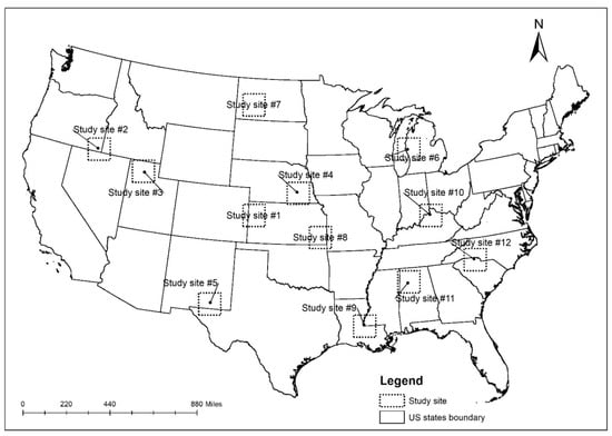
Figure 1.
Locations of the twelve study sites.
Table 3.
Two levels of the classification scheme (The Level II is from the NLCD 2016 product legend and the class names ending with the (#) symbol are not contained within any of the twelve study sites).
Table 4.
Landscape shape index (LSI) value of twelve study sites.
3.2. Classification Data
The classification map of each study site was extracted from the NLCD 2016 produced from Landsat data at the spatial resolution of 30 m [61]. The classification scheme was assumed to influence the positional effect. Therefore, two classification schemes were utilized in this study (Table 3). Level II represents the NLCD 2016 classification scheme with 15 classes that are common to the twelve study sites [10]. The percentage of the 15 classes at each study site is shown in Table 5. The level 1 classification scheme was created by merging the thematic classes from level II into 8 classes (Table 3). The LSI value and percentage of 8 classes of each study site as shown in Table 4 and Table 6, respectively.
Table 5.
Percentage of each thematic class for the twelve study sites using the level II classification scheme (15 classes).
Table 6.
Percentage of each thematic class for twelve study sites using level I classification scheme (8 classes).
The spatial resolution was also assumed to impact the positional effect. As a result, a series of classification maps at different spatial resolutions for each study site were generated by upscaling the NCLD 2016. Different window sizes, varying from 5 × 5, 10 × 10, 20 × 20 and 30 × 30 pixels, were used to create the classification maps at spatial scales of 150, 300, 600 and 900 m, respectively. Figure 2 shows an example of creating a classification map at a scale of 150 m. The label of a coarser pixel in the upscaled classification map was aggregated based on the majority rule. In other words, the dominant class in the window determined the label of the upscaled pixel. If there was more than one dominant class within the window, the upscaled pixel would be labeled as “unclassified”. This upscaling method was applied to each study site for both levels of the classification scheme.
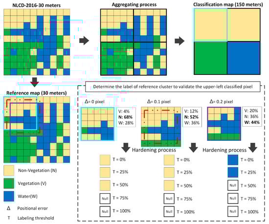
Figure 2.
An example of the classification and the reference data process. In this case, a classification map at the spatial resolution of 150 m was created by aggregation using the majority rule. The classification map has three classes: non-vegetation, vegetation, and water. The upper-left pixel in the classification map was used to compare with a cluster in the reference data where the positional error is 0, 0.1, or 0.2 pixels, respectively. The unique label for the cluster was determined under five distinct labeling thresholds (T).
3.3. Reference Data
The NLCD 2016 product [10] at the spatial resolution of 30 m for the two classification scheme levels, without the introduction of any positional error, was used as the reference data for each study site. Since the same data were used as the map and the reference data in this study, the accuracy between the two data sets is 100% before the simulation of positional error. In this way, thematic errors not caused by positional shifts were completely controlled.
3.4. Accuracy Assessment
In the simulation analysis, the positional error was varied from 0 to 2 pixels in increments of 0.1 pixels. The positional error model was applied to every pixel in the classification map and its corresponding cluster in the reference data. Different labeling thresholds (T) were selected to determine the label of a cluster in the reference data: 0%, 25%, 50%, 75%, and 100%. This research included the threshold of 0% to simulate the scenario in which the simple majority rule was applied to determine the label of a reference cluster [62]. Figure 2 takes the upper-left classified pixel as an example to show how to determine its reference label based on the multiple classes within the cluster due to the positional errors and various labeling thresholds. The spatial resolution of the classification map is 150 m, while that of the reference map is 30 m. The upper-left pixel in the classification map was classified as non-vegetation, but its reference cluster contained multiple classes. The figure presents the steps to determine the label of this reference cluster. If the positional error () was set to 0 pixels, then the proportions of vegetation, non-vegetation, and water within the reference cluster would be 4%, 68%, and 28%, respectively. Therefore, non-vegetation is the dominant class. The reference label was determined as non-vegetation because its proportion in the reference cluster is greater than the labeling threshold (T). If the dominant map class is less than the labeling threshold (T), the reference label is specified as null. In the example in the figure, the reference cluster’s label was specified as non-vegetation when the threshold was set to 0%, 25% or 50%, and null when the threshold was 75% or 100%. This sampling unit (reference cluster) would be abandoned if it was labeled as null. The same calculation was applied to the reference cluster when the positional error was 0.1 pixels and 0.2 pixels, respectively. The labeling result was the same when the positional error was 0.1 pixels, although this amount of positional error slightly changed the class’ proportions. The result was completely different when the positional error reached 0.2 pixels because the dominant class became water with a percentage of 44%. Consequently, if a labeling threshold of 0% or 25% was applied, the reference cluster was labeled as water, otherwise, it was labeled as null and would be abandoned.
To avoid sampling errors, all pixels in the classification map except those labeled as “unclassified” were included in the thematic accuracy assessment. Because the map and the reference data are both generated from the NLCD 2016, the thematic errors shown in the error matrix were only the result of positional errors. The , , , and were recorded between each pair of classification map and reference data for each of the 12 study sites.
4. Results
Figure 3 shows the mean and standard deviation of , , , and (abandoned percentage of assessment units) of the 12 study sites at the four spatial scales and using the eight class classification scheme. The was not presented because its values are zero regardless of the positional errors, spatial scales, and thresholds because simulating positional errors between classification maps and its reference data did not alter the proportions among classes. Figure 3 consists of twenty sub-figures, divided into five groups by rows or four groups by columns. Each row represents a specific labeling threshold (T). The first three columns denote the , , and , respectively, while the last column signifies the . There are four curves representing different scales in each sub-figure. The results found in Figure 3 are detailed below.
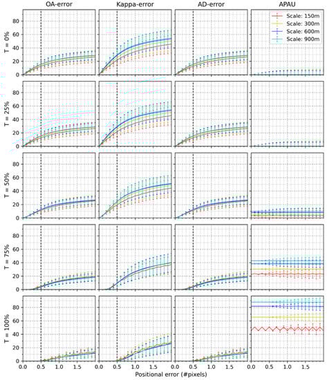
Figure 3.
Mean and standard deviation of , , , and of the twelve study sites at different scales when the classification consists of 8 classes.
- (1)
- The mean value and standard deviation of , , and increase as the positional error grows. and exhibit the same values. at a particular scale (e.g., 150 m) is more significant than and at the same amount of positional error. For example, at the positional error of 1.0 pixels, average are all above 20% as compared to average which are all below 20%. Most values of are relatively stable except for the wavy shape of at the spatial scale of 150 m, with T being 100%.
- (2)
- The average lines of are very close, regardless of thresholds. The same patterns were also found among the lines of and , respectively.
- (3)
- The of the same spatial scale decrease as T rises. The same results are also reflected in either or . For example, when T grows to 100%, the errors in the three accuracy measures approximate 0% if positional errors are under 0.5 pixels. However, the increment in T results in a higher . For example, when the threshold is 0% or 25%, the values of the approach 0. The average lies between 3.46% and 9.84% and between 22.58% and 43.02% when the threshold reaches 50% and 75%, respectively. If T attains 100%, all values of are above 45.29%, with a maximum of 87.93% at a scale of 900 m. The lines of separate from each other if T exceeds 50%.
- (4)
- When the positional error is 0.5 pixels, and T is no more than 50%, , , and are higher than 10%. When the threshold is 75%, and lie between 3.69% and 4.72% while the lie between 8.65% and 9.60%. Nevertheless, over 23.73% of assessment units were abandoned, and the maximum percentage approximates 42.98%. If T is 100%, the , , and drop to 0%, but reaches over 50.72%, and the highest reaches 87.90%.
The results of Figure 3 also hold in Figure 4, where the classification scheme consists of 15 classes. A classification scheme with 15 classes presents higher , , , and compared to 8 classes.
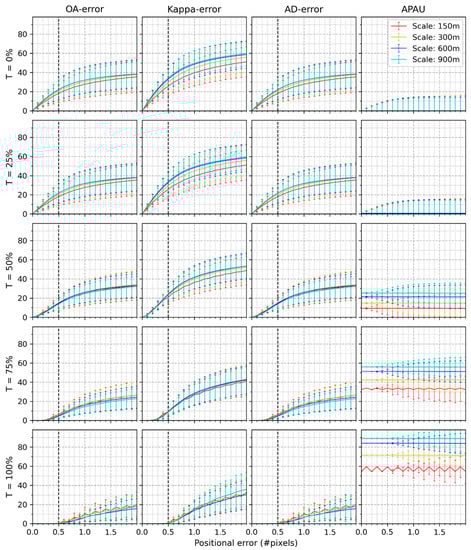
Figure 4.
Mean and standard deviation of , , , and of the twelve study sites at different scales when the classification consists of 15 classes.
Figure 5 shows the mean and standard deviation of , , , and for the four scales at each study site when the classification scheme has eight classes. QD-errors are 0%, and therefore, they are not displayed. The twenty sub-figures were arranged in the same way as for Figure 3 and Figure 4. Twelve curves representing the various study sites exist in each sub-figure. Each curve is an average of four scales. The results found in Figure 5 are listed below.
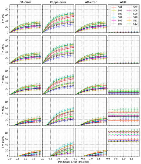
Figure 5.
Mean and standard deviation of , , , and of four spatial scales at different study sites where the classification scheme consists of 8 classes.
- (1)
- The upper-left sub-figure shows that the resulted from positional errors ranging from 0 to 2.0 pixels when T is 0%. Generally, the curve of a study site with a smaller LSI is lower than that of a study site with a larger LSI. For example, the line of study site #5 with an LSI of 367.1 is below that of study site #12 that has an LSI of 438.5. However, this is not true for all study sites. For example, study site #1 holds the minimum LSI (Table 3), yet its line is above that of study site #5.
- (2)
- drop as T grows from 0% to 100%. For example, most of the twelve study sites at the positional error of 0.5 pixels are higher than 10% if T is no more than 50%. When T reaches 75%, are reduced to under 10%. If T exceeds 75%, the drops to 0%.
- (3)
- The same patterns above were found among the study sites using and . However, are more sensitive to positional errors than is the . For instance, with the amount of 2 pixels’ positional errors, all are below 40%. In contrast, approximate 70%.
- (4)
- The values of remain steady compared to , , and . approaches 0% at the thresholds of 0% and 25%. However, lies between 1.12% and 14.55% and between 16.73% and 53.69% when T reaches 50% and 75%, respectively. When T is 100%, the varies between 49.31% and 87.17%.
The patterns found in Figure 6 are similar to those of Figure 5. The only difference is that each line in Figure 6 is higher than the corresponding one in Figure 5 because the classification scheme consists of more classes (15 instead of 8).
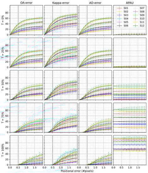
Figure 6.
Mean and standard deviation of , , , and of four spatial scales at different study sites where the classification scheme consists of 15 classes.
5. Discussion
Thematic accuracy assessment aims to measure the classification accuracy of land cover products. However, many uncertainties that exist in the validation procedure could propagate into the error matrix and therefore make the accuracy measures misleading [24,26]. This research examined whether the single-pixel as an assessment unit is appropriate for validating land cover mapping from the perspective of the impacts of positional errors. Twelve study sites, each of which covers a spatial extent of 180 km × 180 km, of different landscape characteristics, were investigated by comparing the NLCD 2016 as the reference data with several coarser classification maps generated from the NLCD 2016 at two classification scheme levels. The results presented the errors in the thematic accuracy measures (overall accuracy, Kappa, allocation disagreement, and quantity disagreement) impacted only by the positional error.
The results showed that overall accuracy, Kappa, and allocation disagreement are very sensitive to positional errors. However, no errors existed in quantity disagreement because either generating coarser classification maps from NLCD 2016 at 30 m or simulating positional errors did not alter the proportions among classes. As a result, the are equal to . Therefore, the following analysis focused on and . There are larger than given the same amount of positional error. The underlying reason is that Kappa adds off-diagonal elements in the error matrix (Table 1) into the calculation as compared to overall accuracy.
Previous studies have not taken the labeling threshold (T) into account, and therefore our research compares directly with these previous studies when T = 0% (the simple majority rule). Using only the majority rule, Powell et al. [27] indicated that over 30% of thematic error was attributed to one pixel’s misregistration using Landsat TM as classification data. Stehman and Wickham [30] proved a conservative bias from 8% to 24% in overall accuracy due to one pixel’s positional error. With the same amount of positional error, this research found that would vary from 20.05% to 23.21% and 27.72% to 32.00% (Figure 3 and Figure 4) using a classification scheme of 8 and 15 classes, respectively. The difference in results between these previous studies and this research results from two factors. First, previous studies performed the experiments at the spatial scale of 30 m, while the scales in this study include 4 spatial scales. Second, they analyzed the effect on accuracy measures when classification and positional errors simultaneously existed. In contrast, the thematic errors in this research only resulted from positional errors, which is more explicit.
This research also demonstrated that a classification map exhibiting more heterogeneous landscape characteristics (Figure 5 and Figure 6) or more classes in a classification scheme (Figure 4 vs. Figure 3) increases the positional effect. These findings are consistent with results in Gu et al. [26]. A coarser spatial scale results in a higher positional effect (Figure 3 or Figure 4) because of a higher proportion of mixed pixels, as shown in Figure 7. The average error lines and associated error bars tend to overlap each other, especially at scales of 600 and 900 m. The underlying reason is that over 50% of the pixels in half of the study sites at the spatial scale of 150 m are mixed and that the mixed proportion increases with higher heterogeneity and coarser scale (Figure 7). In other words, the effect of spatial scale increases as it becomes coarser because most pixels in the classification map are mixed. Increasing the labeling threshold, T, reduces the errors in the accuracy measures; however, it increases the number of sample units that are abandoned () (Figure 3, Figure 4, Figure 5 and Figure 6). Because half-pixel geo-registration accuracy has been achieved and reported in most moderate resolution remote sensing applications [44,45], this research emphasized the thematic errors at the positional error of 0.5 pixels. The and are above 10% at the positional error of 0.5 pixels if T is no more than 50%. The and decrease to below 10% and even down to 0% if T exceeds 50%; however, over 30% of assessment units were abandoned at the three coarser scales (Figure 3), or nine study sites (Figure 5) when the 8 class map was used. The abandoned proportion exceeds 60% when T is 100%. This phenomenon is more severe in the 15 class map (Figure 4 and Figure 6). These results demonstrate that the labeling threshold does not work for thematic accuracy assessment using single-pixel as an assessment unit.
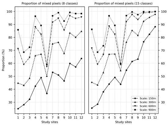
Figure 7.
The proportion of mixed pixels of twelve study sites at different spatial scales.
Global land cover mapping has favored pixel-based classification and the use of a single-pixel as an assessment unit [63,64,65]. Table 7 shows several common global land cover products that were created at a variety of spatial resolutions ranging from 300 to 1000 m. The achieved positional accuracy highly depended on the remote sensing sensor [63,66,67]. The global land cover datasets of IGBP, UMD, and GLC 2000 were created at the spatial resolution of 1000 m and validated using the Landsat TM and SPOT images as reference data [24,64]. The positional accuracy achieved 1 pixel, 1 pixel, and 0.3–0.47 pixels, respectively, relative to their spatial resolutions. The average was 31.92%, 31.92%, and 15.06–18.92%, according to the data (16 classes, 900 m) shown in Figure 4. The average was 49.56%, 49.56%, and 23.08%–29.07%. The advent of medium-resolution sensors such as MODIS and MEdium Resolution Imaging Spectrometer (MERIS) has allowed researchers to map the Earth’s surface at a spatial scale of 500 or 300 m [68,69]. Meanwhile, these sensors have achieved sub-pixel geolocation accuracy [70]. This research analyzed potential errors in accuracy measure using the positional accuracy of MCD12 because of its highest positional accuracy (0.1–0.2 pixel) at the spatial scale of 500 m. Even so, the and would averagely vary from 5.5% to 10.4% and from 8.21% to 15.57%, respectively, according to the data (16 classes, 600 m) in Figure 4. The potential average and in GlobCover would be 13.56% and 19.71%, respectively, in terms of Figure 4 (16 classes, 300 m). It is worth noting that there were more classes in these global land cover products, which means the actual thematic errors would be more severe. Therefore, from the perspective of the positional effect, using a single-pixel as an assessment unit is not appropriate for thematic accuracy assessment. The errors in accuracy measures in this research were only induced by positional errors. However, in reality, there are other sources of errors such as sampling and interpretation errors that would add to the uncertainties evident in the error matrix [12,18,24,27]. The combined effect would further strengthen our conclusion.
Table 7.
Thematic accuracy and positional accuracy of the selected global land cover database.
The choice of an assessment unit for the per-pixel classification accuracy assessment used by remote sensing analysts includes a single pixel, a cluster of pixels (e.g., 3 × 3 pixels), and a polygon [12]. This research complemented the research of [27,30] using twelve study sites of various landscape characteristics under multiple cofactors. This research further confirmed that even if the image achieved half-pixel registration accuracy, choosing a single-pixel as the assessment unit is an inferior choice. However, using a cluster or polygon may generate new questions such as how to sample, compare, and then present the error matrix [30], which needs further research.
This research also has several limitations. First, we assumed a uniform spatial distribution for positional errors. Future work should consider the different forms of geometric distortions and evaluate the worst effect [40]. Second, the twelve study sites using the level I classification scheme were created by collapsing the classes in the stratified random level II study sites. Therefore, while the level II sites were selected to be representative of the landscape characteristics, there was no guarantee that the sites would remain so when collapsed to leve1 I. However, a preliminary analysis shows that the LSI of twelve study sites at level I (Table 3) still covers the dynamic range according to the histogram of LSI (Figure 8). Third, this research only took into account the spatial scales ranging from 150 to 900 m of the classification map, which is limited by the spatial resolution of the NLCD 2016 as reference data. However, if considering the relative size of pixels between the simulated classification map and the reference data, the conclusions could be extended to other spatial scales. Unfortunately, as the spatial resolution increases, it is more challenging to geo-register a pixel to sub-pixel level due to a lack of a high precision digital elevation model [12,71]. Therefore, this research speculates that using a single-pixel as an assessment unit is also not appropriate for thematic accuracy assessment at higher spatial scales. Finally, this research only included twelve study sites within the United States, and all accuracy measures were at the map level. However, this research took 1488 h of processing time using a laptop workstation with an E-2176M 6 core processor and 32 GB of memory. Future work could test the conclusion at a categorical level.
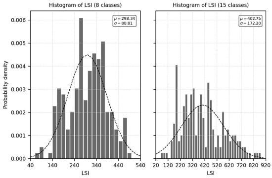
Figure 8.
Histogram of LSI values of 197 grids within the United States.
6. Conclusions
Choosing an assessment unit is a crucial component of the framework of thematic accuracy assessment. There are various choices for the assessment unit, including a single pixel, a cluster of pixels, and a polygon. The main argument lies in whether the single-pixel as an assessment unit is appropriate for thematic accuracy assessment. This research conducted a simulation analysis from the perspective of positional errors. Other factors, including landscape characteristics, classification schemes, spatial scale, and labeling thresholds, were also analyzed. The results showed that the single-pixel as an assessment unit is not appropriate for use in a thematic accuracy assessment. A classification map with a more heterogeneous landscape or more classes in a classification scheme increases the positional effect. The spatial scale has greater impact when most pixels in the classification map are mixed. Increasing the labeling threshold reduces the positional impact; however, it increases the number of assessment units that must be abandoned. Careful consideration of the issues and analysis described in this paper will result in improved thematic accuracy assessment in the future.
Author Contributions
J.G. and R.G.C. conceived and designed the experiments. J.G. performed the experiments and analyzed the data with guidance from R.G.C.; J.G. wrote the paper. R.G.C. edited and finalized the paper and manuscript. All authors have read and agreed to the published version of the manuscript.
Funding
Partial funding was provided by the New Hampshire Agricultural Experiment Station. This is Scientific Contribution Number: #2858. This work was supported by the USDA National Institute of Food and Agriculture McIntire Stennis Project #NH00095-M (Accession #1015520).
Conflicts of Interest
The authors declare no conflict of interest.
References
- Wulder, M.A.; Coops, N.C.; Roy, D.; White, J.C.; Hermosilla, T. Land cover 2.0. Int. J. Remote. Sens. 2018, 39, 4254–4284. [Google Scholar] [CrossRef]
- Giri, C.; Pengra, B.; Long, J.; Loveland, T. Next generation of global land cover characterization, mapping, and monitoring. Int. J. Appl. Earth Obs. Geoinf. 2013, 25, 30–37. [Google Scholar] [CrossRef]
- Wu, C.; Hou, X.; Peng, D.; Gonsamo, A.; Xu, S. Land surface phenology of China’s temperate ecosystems over 1999–2013: Spatial–temporal patterns, interaction effects, covariation with climate and implications for productivity. Agric. For. Meteorol. 2016, 216, 177–187. [Google Scholar] [CrossRef]
- Xin, Q.; Broich, M.; Zhu, P.; Gong, P. Modeling grassland spring onset across the Western United States using climate variables and MODIS-derived phenology metrics. Remote Sens. Environ. 2015, 161, 63–77. [Google Scholar] [CrossRef]
- Defourny, P.; D’Andrimont, R.; Maugnard, A.; Defourny, P. Survey of Hyperspectral Earth Observation Applications from Space in the Sentinel-2 Context. Remote Sens. 2018, 10, 157. [Google Scholar] [CrossRef]
- Abdi, A. Land cover and land use classification performance of machine learning algorithms in a boreal landscape using Sentinel-2 data. GISci. Remote Sens. 2020, 57, 1–20. [Google Scholar] [CrossRef]
- Homer, C.; Xian, G.; Jin, S.; Wickham, J.D.; Costello, C.; Danielson, P.; Gass, L.; Funk, M.; Stehman, S.V.; Stehman, S.; et al. Conterminous United States land cover change patterns 2001–2016 from the 2016 National Land Cover Database. ISPRS J. Photogramm. Remote Sens. 2020, 162, 184–199. [Google Scholar] [CrossRef]
- Bartholomé, E.; Belward, A.S. GLC2000: A new approach to global land cover mapping from Earth observation data. Int. J. Remote Sens. 2005, 26, 1959–1977. [Google Scholar] [CrossRef]
- Teluguntla, P.; Thenkabail, P.; Xiong, J.; Gumma, M.K.; Giri, C.; Milesi, C.; Ozdogan, M.; Congalton, R.; Tilton, J.; Sankey, T.; et al. Global Food Security Support Analysis Data (GFSAD) at Nominal 1-km (GCAD) derived from Remote Sensing in Support of Food Security in the Twenty-first Century: Current Achievements and Future Possibilities. In Remote Sensing Handbook, 1st ed.; Teluguntla, P., Thenkabail, P., Eds.; CRC/Taylor & Francis: Boca Raton, FL, USA, 2016; Volume II, pp. 131–159. [Google Scholar]
- Wickham, J.D.; Stehman, S.V.; Gass, L.; Dewitz, J.A.; Sorenson, D.G.; Granneman, B.J.; Poss, R.V.; Baer, L.A. Thematic accuracy assessment of the 2011 National Land Cover Database (NLCD). Remote Sens. Environ. 2017, 191, 328–341. [Google Scholar] [CrossRef]
- Tchuenté, A.T.K.; Roujean, J.-L.; De Jong, S.M. Comparison and relative quality assessment of the GLC2000, GLOBCOVER, MODIS and ECOCLIMAP land cover data sets at the African continental scale. Int. J. Appl. Earth Obs. Geoinf. 2011, 13, 207–219. [Google Scholar] [CrossRef]
- Congalton, R.G.; Green, K. Assessing the Accuracy of Remotely Sensed Data: Principles and Practices; CRC Press: Boca Raton, FL, USA, 2019. [Google Scholar]
- Morales-Barquero, L.; Lyons, M.B.; Phinn, S.R.; Roelfsema, C.M. Trends in Remote Sensing Accuracy Assessment Approaches in the Context of Natural Resources. Remote Sens. 2019, 11, 2305. [Google Scholar] [CrossRef]
- Stehman, S.V.; Foody, G.M. Key issues in rigorous accuracy assessment of land cover products. Remote Sens. Environ. 2019, 231, 111199. [Google Scholar] [CrossRef]
- Congalton, R.G. A review of assessing the accuracy of classifications of remotely sensed data. Remote Sens. Environ. 1991, 37, 35–46. [Google Scholar] [CrossRef]
- Foody, G.M. Status of land cover classification accuracy assessment. Remote Sens. Environ. 2002, 80, 185–201. [Google Scholar] [CrossRef]
- Foody, G.M. Assessing the accuracy of land cover change with imperfect ground reference data. Remote Sens. Environ. 2010, 114, 2271–2285. [Google Scholar] [CrossRef]
- Plourde, L.; Congalton, R.G. Sampling method and sample placement: How do they affect the accuracy of remotely sensed maps? Photogrammet. Eng. Remote Sens. 2003, 69, 289–297. [Google Scholar] [CrossRef]
- Stehman, S.V. Practical Implications of Design-Based Sampling Inference for Thematic Map Accuracy Assessment. Remote Sens. Environ. 2000, 72, 35–45. [Google Scholar] [CrossRef]
- Story, M.; Congalton, R.G. accuracy assessment—A users perspective. Photogrammetr. Eng. Remote Sens. 1986, 52, 397–399. [Google Scholar]
- Stehman, S.V.; Czaplewski, R.L. Design and Analysis for Thematic Map Accuracy Assessment. Remote Sens. Environ. 1998, 64, 331–344. [Google Scholar] [CrossRef]
- Stehman, S.V. Sampling designs for accuracy assessment of land cover. Int. J. Remote Sens. 2009, 30, 5243–5272. [Google Scholar] [CrossRef]
- Olofsson, P.; Foody, G.M.; Herold, M.; Stehman, S.V.; Woodcock, C.E.; Wulder, M.A. Good practices for estimating area and assessing accuracy of land change. Remote Sens. Environ. 2014, 148, 42–57. [Google Scholar] [CrossRef]
- Congalton, R.G.; Gu, J.; Yadav, K.; Thenkabail, P.S.; Özdoğan, M. Global Land Cover Mapping: A Review and Uncertainty Analysis. Remote Sens. 2014, 6, 12070–12093. [Google Scholar] [CrossRef]
- Gu, J.; Congalton, R.G. The Positional Effect in Soft Classification Accuracy Assessment. Am. J. Remote Sens. 2019, 7, 50. [Google Scholar] [CrossRef]
- Gu, J.; Congalton, R.G.; Pan, Y. The Impact of Positional Errors on Soft Classification Accuracy Assessment: A Simulation Analysis. Remote Sens. 2015, 7, 579–599. [Google Scholar] [CrossRef]
- Powell, R.; Matzke, N.; De Souza, C.; Clark, M.; Numata, I.; Hess, L.; Roberts, D. Sources of error in accuracy assessment of thematic land-cover maps in the Brazilian Amazon. Remote Sens. Environ. 2004, 90, 221–234. [Google Scholar] [CrossRef]
- Nakaegawa, T. Uncertainty in land cover datasets for global land-surface models derived from 1-km global land cover datasets. Hydrol. Process. 2011, 25, 2703–2714. [Google Scholar] [CrossRef]
- Selkowitz, D.J.; Stehman, S.V. Thematic accuracy of the National Land Cover Database (NLCD) 2001 land cover for Alaska. Remote Sens. Environ. 2011, 115, 1401–1407. [Google Scholar] [CrossRef]
- Stehman, S.V.; Wickham, J.D. Pixels, blocks of pixels, and polygons: Choosing a spatial unit for thematic accuracy assessment. Remote Sens. Environ. 2011, 115, 3044–3055. [Google Scholar] [CrossRef]
- Ye, S.; Rakshit, R.G.P., Jr. A review of accuracy assessment for object-based image analysis: From per-pixel to per-polygon approaches. ISPRS J. Photogramm. Remote Sens. 2018, 141, 137–147. [Google Scholar] [CrossRef]
- Radoux, J.; Bogaert, P.; Fasbender, D.; Defourny, P. Thematic accuracy assessment of geographic object-based image classification. Int. J. Geogr. Inf. Sci. 2010, 25, 895–911. [Google Scholar] [CrossRef]
- Chen, G.; Weng, Q.; Hay, G.J.; He, Y. Geographic object-based image analysis (GEOBIA): Emerging trends and future opportunities. GISci. Remote Sens. 2018, 55, 159–182. [Google Scholar] [CrossRef]
- Rakshit, R.G.P., Jr.; Cheuk, M.L. A generalized cross-tabulation matrix to compare soft-classified maps at multiple resolutions. Int. J. Geogr. Inf. Sci. 2006, 20, 1–30. [Google Scholar] [CrossRef]
- Silván-Cárdenas, J.L.; Wang, L. Sub-pixel confusion–uncertainty matrix for assessing soft classifications. Remote Sens. Environ. 2008, 112, 1081–1095. [Google Scholar] [CrossRef]
- Janssen, L.L.F.; Vanderwel, F.J.M. Accuracy assessment of satellite-derived land-cover data—A review. Photogrammetr. Eng. Remote Sens. 1994, 60, 419–426. [Google Scholar]
- Richards, J.A. Classifier performance and map accuracy. Remote Sens. Environ. 1996, 57, 161–166. [Google Scholar] [CrossRef]
- Wickham, J.D.; Stehman, S.; Fry, J.; Smith, J.; Homer, C. Thematic accuracy of the NLCD 2001 land cover for the conterminous United States. Remote Sens. Environ. 2010, 114, 1286–1296. [Google Scholar] [CrossRef]
- Heydari, S.S.; Mountrakis, G. Effect of classifier selection, reference sample size, reference class distribution and scene heterogeneity in per-pixel classification accuracy using 26 Landsat sites. Remote Sens. Environ. 2018, 204, 648–658. [Google Scholar] [CrossRef]
- Brown, K.M.; Foody, G.M.; Atkinson, P.M. Modelling geometric and misregistration error in airborne sensor data to enhance change detection. Int. J. Remote Sens. 2007, 28, 2857–2879. [Google Scholar] [CrossRef]
- Eastman, R.D.; Le Moigne, J.; Netanyahu, N.S. Research issues in image registration for remote sensing. In Proceedings of the 2007 IEEE Conference on Computer Vision and Pattern Recognition, Minneapolis, MN, USA, 17–22 June 2007; Volume 1–8, pp. 1–8. [Google Scholar]
- Congalton, R.G. Thematic and Positional Accuracy Assessment of Digital Remotely Sensed Data. In Proceedings of the Seventh Annual Forest Inventory and Analysis Symposium, Portland, ME, USA, 3–6 October 2005; McRoberts, R.E., Reams, G.A., Van Deusen, P.C., McWilliams, W.H., Eds.; US Department of Agriculture, Forest Service: Washington, DC, USA, 2005; pp. 149–154. [Google Scholar]
- Aguilar, M.A.; Agüera, F.; Aguilar, F.J.; Carvajal, F.; Carvajal-Ramírez, F. Geometric accuracy assessment of the orthorectification process from very high resolution satellite imagery for Common Agricultural Policy purposes. Int. J. Remote Sens. 2008, 29, 7181–7197. [Google Scholar] [CrossRef]
- Benediktsson, J.A.; Tan, B.; Woodcock, C.E.; Stone, H.S.; Chen, Q.-S.; Cole-Rhodes, A.A.; Varshney, P.K.; Goshtasby, A.A.; Mount, D.M.; Ratanasanya, S.; et al. Image Registration for Remote Sensing; Cambridge University Press (CUP): Cambridge, UK, 2009. [Google Scholar]
- Keshtkar, H.; Voigt, W.; Alizadeh, E. Land-cover classification and analysis of change using machine-learning classifiers and multi-temporal remote sensing imagery. Arab. J. Geosci. 2017, 10, 154. [Google Scholar] [CrossRef]
- McRoberts, R.E. The effects of rectification and Global Positioning System errors on satellite image-based estimates of forest area. Remote Sens. Environ. 2010, 114, 1710–1717. [Google Scholar] [CrossRef]
- Verbyla, D.L.; Hammond, T.O. Conservative bias in classification accuracy assessment due to pixel-by-pixel comparison of classified images with reference grids. Int. J. Remote Sens. 1995, 16, 581–587. [Google Scholar] [CrossRef]
- Smith, J.H.; Stehman, S.V.; Wickham, J.D.; Yang, L. Effects of landscape characteristics on land-cover class accuracy. Remote Sens. Environ. 2003, 84, 342–349. [Google Scholar] [CrossRef]
- Belgiu, M.; Drăguţ, L. Random forest in remote sensing: A review of applications and future directions. ISPRS J. Photogramm. Remote Sens. 2016, 114, 24–31. [Google Scholar] [CrossRef]
- Mountrakis, G.; Im, J.; Ogole, C. Support vector machines in remote sensing: A review. ISPRS J. Photogramm. Remote Sens. 2011, 66, 247–259. [Google Scholar] [CrossRef]
- Dai, X.; Khorram, S. The effects of image misregistration on the accuracy of remotely sensed change detection. IEEE Trans. Geosci. Remote Sens. 1998, 36, 1566–1577. [Google Scholar] [CrossRef]
- Chen, G.; Zhao, K.; Powers, R. Assessment of the image misregistration effects on object-based change detection. ISPRS J. Photogramm. Remote Sens. 2014, 87, 19–27. [Google Scholar] [CrossRef]
- Rakshit, R.G.P., Jr.; Millones, M. Death to Kappa: Birth of quantity disagreement and allocation disagreement for accuracy assessment. Int. J. Remote Sens. 2011, 32, 4407–4429. [Google Scholar] [CrossRef]
- Warrens, M.J. Properties of the quantity disagreement and the allocation disagreement. Int. J. Remote Sens. 2015, 36, 1439–1446. [Google Scholar] [CrossRef]
- Chen, J.; Chen, J.; Liao, A.; Cao, X.; Chen, L.; Chen, X.; He, C.; Han, G.; Peng, S.; Lu, M.; et al. Global land cover mapping at 30m resolution: A POK-based operational approach. ISPRS J. Photogramm. Remote Sens. 2015, 103, 7–27. [Google Scholar] [CrossRef]
- Liu, X.; Hu, G.; Chen, Y.; Li, X.; Xu, X.; Li, S.; Pei, F.; Wang, S. High-resolution multi-temporal mapping of global urban land using Landsat images based on the Google Earth Engine Platform. Remote Sens. Environ. 2018, 209, 227–239. [Google Scholar] [CrossRef]
- Wang, J.; Zhao, Y.; Li, C.; Yu, L.; Liu, D.; Gong, P. Mapping global land cover in 2001 and 2010 with spatial-temporal consistency at 250m resolution. ISPRS J. Photogramm. Remote Sens. 2015, 103, 38–47. [Google Scholar] [CrossRef]
- Schwaller, M.R.; Southwell, C.; Emmerson, L. Continental-scale mapping of Adélie penguin colonies from Landsat imagery. Remote Sens. Environ. 2013, 139, 353–364. [Google Scholar] [CrossRef]
- Yang, L.; Jin, S.; Danielson, P.; Homer, C.; Gass, L.; Bender, S.M.; Case, A.; Costello, C.; Dewitz, J.; Fry, J.; et al. A new generation of the United States National Land Cover Database: Requirements, research priorities, design, and implementation strategies. ISPRS J. Photogramm. Remote Sens. 2018, 146, 108–123. [Google Scholar] [CrossRef]
- McGarigal, K.; Marks, B.J. FRAGSTATS: Spatial pattern analysis program for quantifying landscape structure., PNW-GTR-351. Portland, OR: U.S. Department of Agriculture, Forest Service, Pacific Northwest Research Station. Gen. Tech. Rep. 1995, 122, 351. [Google Scholar]
- Wickham, J.D.; Stehman, S.V.; Gass, L.; Dewitz, J.; Fry, J.A.; Wade, T.G. Accuracy assessment of NLCD 2006 land cover and impervious surface. Remote Sens. Environ. 2013, 130, 294–304. [Google Scholar] [CrossRef]
- Mayaux, P.; Eva, H.; Gallego, J.; Strahler, A.H.; Herold, M.; Agrawal, S.; Naumov, S.; De Miranda, E.E.; Di Bella, C.M.; Ordoyne, C.; et al. Validation of the global land cover 2000 map. IEEE Trans. Geosci. Remote Sens. 2006, 44, 1728–1739. [Google Scholar] [CrossRef]
- Brovelli, M.A.; Molinari, M.E.; Hussein, E.; Chen, J.; Li, R. The First Comprehensive Accuracy Assessment of GlobeLand30 at a National Level: Methodology and Results. Remote Sens. 2015, 7, 4191–4212. [Google Scholar] [CrossRef]
- Zhao, Y.; Gong, P.; Yu, L.; Hu, L.; Li, X.; Li, C.; Zhang, H.; Zheng, Y.; Wang, J.; Zhao, Y.; et al. Towards a common validation sample set for global land-cover mapping. Int. J. Remote Sens. 2014, 35, 4795–4814. [Google Scholar] [CrossRef]
- Kuenzer, C.; Leinenkugel, P.; Vollmuth, M.; Dech, S. Comparing global land-cover products—Implications for geoscience applications: An investigation for the trans-boundary Mekong Basin. Int. J. Remote Sens. 2014, 35, 2752–2779. [Google Scholar] [CrossRef]
- Bicheron, P.; Amberg, V.; Bourg, L.; Petit, D.; Huc, M.; Miras, B.; Hagolle, O.; Delwart, S.; Ranera, F.; Arino, O.; et al. Geolocation Assessment of MERIS GlobCover Orthorectified Products. IEEE Trans. Geosci. Remote Sens. 2011, 49, 2972–2982. [Google Scholar] [CrossRef]
- Sylvander, S.; Albert-Grousset, I.; Henry, P. Geometrical performance of the VEGETATION products. In Proceedings of the IGARSS 2003. 2003 IEEE International Geoscience and Remote Sensing Symposium. Proceedings (IEEE Cat. No.03CH37477), Toulouse, France, 21–25 July 2004; Volume 571, pp. 573–575. [Google Scholar]
- Sulla-Menashe, D.; Gray, J.M.; Abercrombie, S.P.; Friedl, M.A. Hierarchical mapping of annual global land cover 2001 to present: The MODIS Collection 6 Land Cover product. Remote Sens. Environ. 2019, 222, 183–194. [Google Scholar] [CrossRef]
- Tateishi, R.; Uriyangqai, B.; Al-Bilbisi, H.; Ghar, M.A.; Tsend-Ayush, J.; Kobayashi, T.; Kasimu, A.; Hoan, N.T.; Shalaby, A.; Alsaaideh, B.; et al. Production of global land cover data—GLCNMO. Int. J. Digit. Earth 2011, 4, 22–49. [Google Scholar] [CrossRef]
- Wolfe, R.E.; Nishihama, M.; Fleig, A.J.; Kuyper, J.A.; Roy, D.P.; Storey, J.C.; Patt, F.S. Achieving sub-pixel geolocation accuracy in support of MODIS land science. Remote Sens. Environ. 2002, 83, 31–49. [Google Scholar] [CrossRef]
- Davis, C.; Wang, X. High resolution DEMs for urban applications. In Proceedings of the IGARSS 2000. IEEE 2000 International Geoscience and Remote Sensing Symposium. Taking the Pulse of the Planet: The Role of Remote Sensing in Managing the Environment. Proceedings (Cat. No.00CH37120), Honolulu, HI, USA, 24–28 July 2002; Volume 2887, pp. 2885–2889. [Google Scholar]
- Husak, G.J.; Hadley, B.C.; McGwire, K.C. Landsat thematic mapper registration accuracy and its effects on the IGBP validation. Photogrammetr. Eng. Remote Sens. 1999, 65, 1033–1039. [Google Scholar]
- Loveland, T.R.; Reed, B.C.; Brown, J.F.; Ohlen, D.O.; Zhu, Z.; Yang, L.; Merchant, J.W. Development of a global land cover characteristics database and IGBP DISCover from 1 km AVHRR data. Int. J. Remote Sens. 2000, 21, 1303–1330. [Google Scholar] [CrossRef]
- McCallum, I.; Obersteiner, M.; Nilsson, S.; Shvidenko, A. A spatial comparison of four satellite derived 1km global land cover datasets. Int. J. Appl. Earth Obs. Geoinf. 2006, 8, 246–255. [Google Scholar] [CrossRef]
- Hansen, M.C.; DeFries, R.S.; Townshend, J.R.G.; Sohlberg, R.A. Global land cover classification at 1 km spatial resolution using a classification tree approach. Int. J. Remote Sens. 2000, 21, 1331–1364. [Google Scholar] [CrossRef]
- Sylvander, S.; Henry, P.; Bastien-Thiry, C.; Meunier, F.; Fuster, D. VEGETATION geometrical image quality. Bulletin de la Société Française de Photogrammétrie et de Télédétection 2000, 159, 59–65. [Google Scholar]
- Shirahata, L.M.; Iizuka, K.; Yusupujiang, A.; Rinawan, F.R.; Bhattarai, R.; Dong, X. Production of Global Land Cover Data–GLCNMO2013. J. Geograph. Geol. 2017, 9, 1–15. [Google Scholar]
- Defourny, P.; Bontemps, S.; Obsomer, V.; Schouten, L.; Bartalev, S.; Herold, M.; Bicheron, P.; Bogaert, E.; Leroy, M.; Arino, O. Accuracy assessment of global land cover maps: Lessons learnt from the GlobCover and GlobCorine Experiences. In Proceedings of the 2010 European Space Agency Living Planet Symposium, Bergen, Norway, 28 June–2 July 2010. [Google Scholar]


Publisher’s Note: MDPI stays neutral with regard to jurisdictional claims in published maps and institutional affiliations. |
© 2020 by the authors. Licensee MDPI, Basel, Switzerland. This article is an open access article distributed under the terms and conditions of the Creative Commons Attribution (CC BY) license (http://creativecommons.org/licenses/by/4.0/).