Estimation of Vertical Datum Parameters Using the GBVP Approach Based on the Combined Global Geopotential Models

 , ,
, ,
Abstract
:
1. Introduction
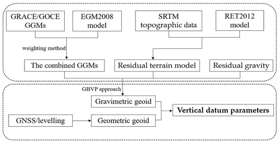
2. Methods
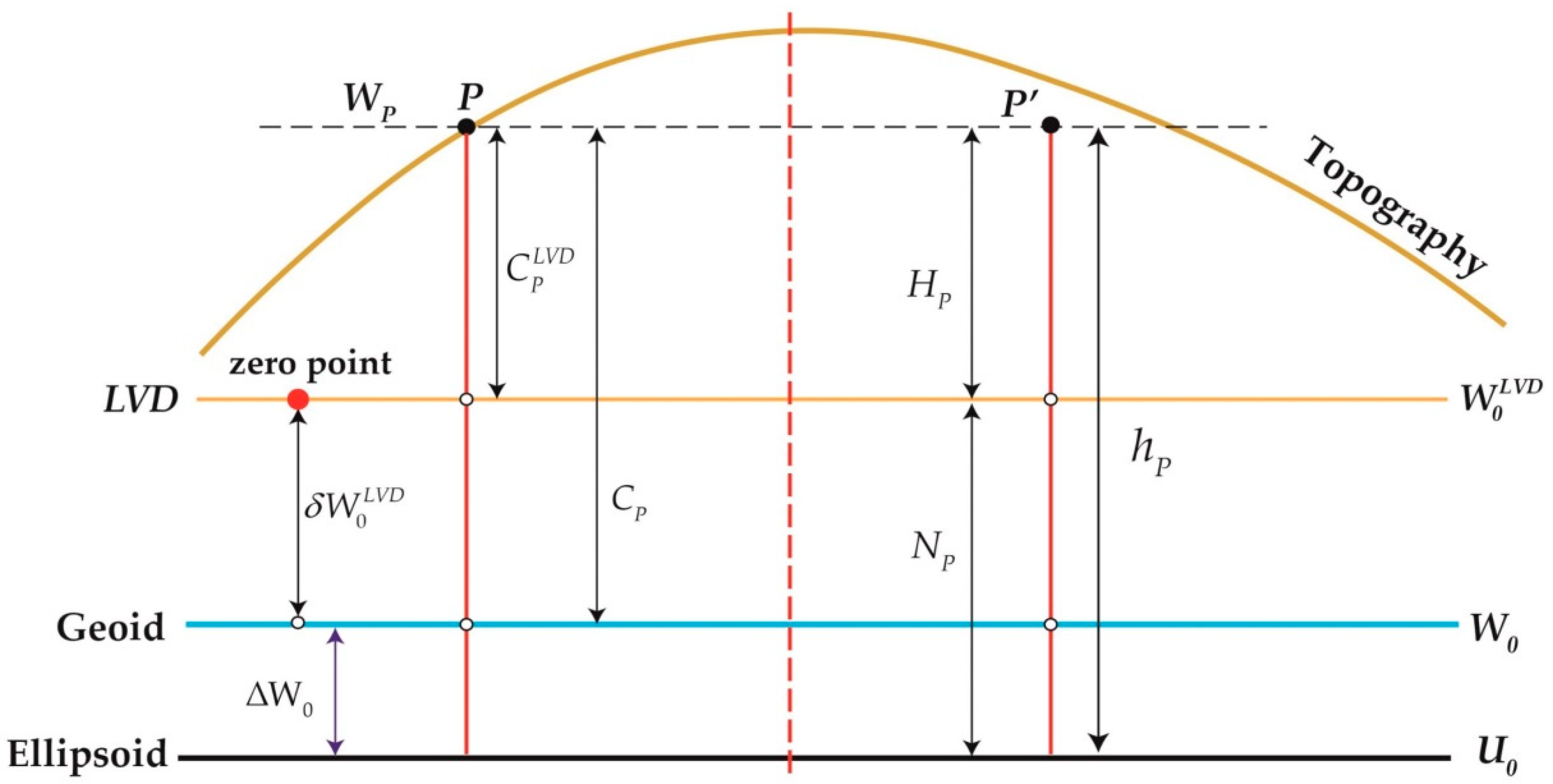
2.1. Determination of the Vertical Datum Parameters Based on the Geodetic Boundary Value Problem (GBVP) Approach
2.2. Determination of the Combined Global Geopotential Models (GGMs) by the Weighting Method
3. Data Sets
3.1. Global Geopotential Models (GGMs)
3.2. GNSS/Levelling Data
3.3. Gravity Data
3.4. Topographic Data
4. Results
4.1. Spectral Accuracy Evaluation of the GGMs
4.2. Omission Errors of the GGMs
4.3. Effect of the Indirect Bias Term
4.4. Determination the Combined GGM
4.5. Residual Gravity Anomalies
4.6. Estimation of Vertical Datum Parameters
5. Conclusions
Author Contributions
Funding
Acknowledgments
Conflicts of Interest
References
- Filmer, M.S.; Hughes, C.W.; Woodworth, P.L.; Featherstone, W.E.; Bingham, R.J. Comparison between geodetic and oceanographic approaches to estimate mean dynamic topography for vertical datum unification: Evaluation at Australian tide gauges. J. Geod. 2018, 92, 1–25. [Google Scholar] [CrossRef] [Green Version]
- Vu, D.T.; Bruinsma, S.; Bonvalot, S.; Remy, D.; Vergos, G.S. A Quasigeoid-Derived Transformation Model Accounting for Land Subsidence in the Mekong Delta towards Height System Unification in Vietnam. Remote Sens. 2020, 12, 817. [Google Scholar] [CrossRef] [Green Version]
- Drewes, H.; Kuglitsch, F.; Adám, J.; Rózsa, S. The Geodesist’s Handbook 2016. J. Geod. 2016, 90, 907–1205. [Google Scholar] [CrossRef]
- Ihde, J.; Sánchez, L.; Barzaghi, R.; Drewes, H.; Foerste, C.; Gruber, T.; Liebsch, G.; Marti, U.; Pail, R.; Sideris, M. Definition and proposed realization of the international height reference system (IHRS). Surv. Geophys. 2017, 38, 549–570. [Google Scholar] [CrossRef]
- Sánchez, L.; Sideris, M.G. Vertical datum unification for the International Height Reference System (IHRS). Geophys. J. Int. 2017, 209, 570–586. [Google Scholar] [CrossRef]
- Thompson, K.R.; Huang, J.; Véronneau, M.; Wright, D.G.; Lu, Y. Mean surface topography of the northwest Atlantic: Comparison of estimates based on satellite, terrestrial gravity, and oceanographic observations. J. Geophys. Res. 2009, 114, C07015. [Google Scholar] [CrossRef] [Green Version]
- Woodworth, P.L.; Hughes, C.W.; Bingham, R.J.; Gruber, T. Towards worldwide height system unification using ocean information. J. Geod. Sci. 2012, 2, 302–318. [Google Scholar] [CrossRef] [Green Version]
- Gomez, M.E.; Pereira, R.A.D.; Ferreira, V.G.; Del Cogliano, D.; Luz, R.T.; De Freitas, S.R.C.; Farias, C.; Perdomo, R.; Tocho, C.; Lauria, E.; et al. Analysis of the Discrepancies Between the Vertical Reference Frames of Argentina and Brazil. In IAG 150 Years; Rizos, C., Willis, P., Eds.; Springer International Publishing: Cham, Switzerland, 2015; Volume 143, pp. 289–295. [Google Scholar]
- Tocho, C.; Vergos, G.S. Estimation of the Geopotential Value W0 for the Local Vertical Datum of Argentina Using EGM2008 and GPS/Levelling Data. In IAG 150 Years; Rizos, C., Willis, P., Eds.; Springer International Publishing: Cham, Switzerland, 2015; Volume 143, pp. 271–279. [Google Scholar]
- He, L.; Chu, Y.H.; Xu, X.Y.; TengXu, Z. Evaluation of the GRACE/GOCE Global Geopotential Model on estimation of the geopotential value for the China vertical datum of 1985. Chin. J. Geophys. 2019, 62, 2016–2026. [Google Scholar]
- Colombo, O. A World Vertical Network. OSU Report No. 296; The Ohio State University: Columbus, OH, USA, 1980. [Google Scholar]
- Rummel, R.; Teunissen, P. Height datum definition, height datum connection and the role of the geodetic boundary value problem. Bull. Geod. 1988, 62, 477–498. [Google Scholar] [CrossRef]
- Zhang, L.; Li, F.; Chen, W.; Zhang, C. Height datum unification between Shenzhen and Hong Kong using the solution of the linearized fixed-gravimetric boundary value problem. J. Geod. 2009, 83, 411–417. [Google Scholar] [CrossRef]
- Amjadiparvar, B.; Rangelova, E.; Sideris, M.G. The GBVP approach for vertical datum unification: Recent results in North America. J. Geod. 2016, 90, 45–63. [Google Scholar] [CrossRef]
- Ebadi, A.; Ardalan, A.; Karimi, R. The Iranian height datum offset from the GBVP solution and spirit-leveling/gravimetry data. J. Geod. 2019, 93, 1207–1225. [Google Scholar] [CrossRef]
- Rülke, A.; Liebsch, G.; Sacher, M.; Schäfer, U.; Schirmer, U.; Ihde, J. Unification of European height system realizations. J. Geod. Sci. 2012, 2, 343–354. [Google Scholar] [CrossRef]
- Sansò, F.; Sideris, M.G. Geoid Determination; Springer: Berlin/Heidelberg, Germany, 2013. [Google Scholar]
- Barzaghi, B. The Remove-Restore Method. In Encyclopedia of Geodesy; Springer International Publishing: Cham, Switzerland, 2015; pp. 1–4. [Google Scholar]
- Gruber, T.; Visser, P.; Ackermann, C.; Hosse, M. Validation of GOCE gravity field models by means of orbit residuals and geoid comparisons. J. Geod. 2011, 85, 845–860. [Google Scholar] [CrossRef]
- Rummel, R. Height unification using GOCE. J. Geod. Sci. 2012, 2, 355–362. [Google Scholar] [CrossRef]
- Tziavos, I.N.; Vergos, G.S.; Grigoriadis, V.N.; Tzanou, E.A.; Natsiopoulos, D.A. Validation of GOCE/GRACE Satellite Only and Combined Global Geopotential Models Over Greece in the Frame of the GOCESeaComb Project. In IAG 150 Years; Rizos, C., Willis, P., Eds.; Springer International Publishing: Cham, Switzerland, 2015; Volume 143, pp. 297–304. [Google Scholar]
- Sánchez, L.; Sideris, M.; Ihde, J. Activities and Plans of the GGOS Focus Area Unified Height System; IUGG General Assembly: Montreal, QC, Canada, 2019. [Google Scholar]
- Forsberg, R.; Tscherning, C. The use of height data in gravity field approximation by collocation. J. Geophys. Res. 1981, 86, 7843–7854. [Google Scholar] [CrossRef]
- Forsberg, R. A Study of Terrain Reductions, Density Anomalies and Geophysical Inversion Methods in Gravity Field Modelling; Technical report; The Ohio State University: Colombus, OH, USA, 1984. [Google Scholar]
- Hirt, C.; Featherstone, W.E.; Marti, U. Combining EGM2008 and SRTM/DTM2006.0 Residual Terrain Model Data to improve Quasigeoid Computations in Mountainous Areas Devoid of Gravity Data. J. Geod. 2010, 84, 557–567. [Google Scholar] [CrossRef] [Green Version]
- Rexer, M.; Hirt, C.; Bucha, B.; Holmes, S. Solution to the spectral filter problem of residual terrain modelling (RTM). J. Geod. 2017, 92, 675–690. [Google Scholar] [CrossRef]
- Hirt, C.; Bucha, M.; Yang, M.; Kuhn, M. A numerical study of residual terrain modelling (RTM) techniques and the harmonic correction using ultra-high degree spectral gravity modelling. J. Geod. 2019, 93, 1469–1486. [Google Scholar] [CrossRef]
- Heiskanen, W.A.; Moritz, H. Physical Geodesy; W.H. Freeman and Company: San Francisco, CA, USA, 1967. [Google Scholar]
- Moritz, H. Geodetic Reference System 1980. J. Geod. 2000, 74, 128–133. [Google Scholar] [CrossRef]
- Gerlach, C.; Rummel, R. Global height system unification with GOCE: A simulation study on the indirect bias term in the GBVP approach. J. Geod. 2013, 87, 57–67. [Google Scholar] [CrossRef]
- Grombein, T.; Seitz, K.; Heck, B. Height system unification based on the fixed GBVP approach. In IAG 150 Years; Rizos, C., Willis, P., Eds.; Springer International Publishing: Cham, Switzerland, 2015; Volume 143, pp. 305–311. [Google Scholar]
- Hayden, T.; Amjadiparvar, B.; Rangelova, E.; Sideris, M.G. Estimating Canadian vertical datum offsets using GNSS/levelling benchmark information and GOCE global geopotential models. J. Geod. Sci. 2012, 2, 257–269. [Google Scholar] [CrossRef] [Green Version]
- Grombein, T.; Seitz, K.; Heck, B. On High-Frequency Topography-Implied Gravity Signals For a Height System Unification Using GOCE-based Global Geopotential Models. Surv. Geophys. 2016, 38, 1–35. [Google Scholar] [CrossRef]
- Pavlis, N.K.; Holmes, S.A.; Kenyon, S.C.; Factor, J.K. The development and evaluation of the earth gravitational model 2008 (EGM2008). J. Geophys. Res. 2012, 117, B04406. [Google Scholar] [CrossRef] [Green Version]
- Wenzel, H.G. Geoid computation by least squares spectral combination using integral formulas. In Proceedings of the IAG General Meeting, Tokyo, Japan, 7–15 May 1982; pp. 438–453. [Google Scholar]
- Gilardoni, R.; Reguzzoni, M.; Sampietro, D. GECO: A global gravity model by locally combining GOCE data and EGM2008. Stud. Geophys Geod. 2016, 60, 228–247. [Google Scholar] [CrossRef]
- Gerlach, C.; Ophaug, V. Accuracy of Regional Geoid Modelling with GOCE. In International Association of Geodesy Symposia; Springer: Cham, Switzerland, 2017; Volume 148, pp. 17–23. [Google Scholar]
- Förste, C.; Abrykosov, O.; Bruinsma, S.; Dahle, C.; König, R.; Lemoine, J.M. ESA’s Release 6 GOCE Gravity Field Model by Means of the Direct Approach Based on Improved Filtering of the Reprocessed Gradients of the Entire Mission (GO_CONS_GCF_2_DIR_R6). Available online: https://doi.org/10.5880/ICGEM.2019.004 (accessed on 14 May 2020).
- Brockmann, J.M.; Schubert, T.; Torsten, M.G.; Schuh, W.D. The Earth’s Gravity Field as Seen by the GOCE Satellite-An Improved Sixth Release Derived with the Time-Wise Approach (GO_CONS_GCF_2_TIM_R6). Available online: http://doi.org/10.5880/ICGEM.2019.003 (accessed on 14 May 2020).
- Xu, X.; Zhao, Y.; Reubelt, T.; Robert, T. A GOCE only gravity model GOSG01S and the validation of GOCE related satellite gravity models. Geod. Geodyn. 2018, 8, 260–272. [Google Scholar] [CrossRef]
- Wu, H.; Müller, J.; Brieden, P. The IfE global gravity field model from GOCE-only observations. In Proceedings of the International Symposium on Gravity, Geoid and Height Systems, Thessaloníki, Greece, 19–23 September 2016. [Google Scholar]
- Lu, B.; Luo, Z.; Zhong, B.; Zhou, H.; Flechtner, F.; Förste, C.; Barthelmes, F.; Zhou, R. The gravity field model IGGT_R1 based on the second invariant of the GOCE gravitational gradient tensor. J. Geod. 2017, 92, 561–572. [Google Scholar] [CrossRef] [Green Version]
- Gatti, A.; Reguzzoni, M.; Migliaccio, F.; Sansò, F. Computation and assessment of the fifth release of the GOCE-only space-wise solution. In Proceedings of the 1st Joint Commission 2 and IGFS Meeting, Thessaloníki, Greece, 19–23 September 2016. [Google Scholar]
- Sánchez, L.; Ågren, J.; Huang, J.; Wang, Y.M.; Forsberg, R. Basic Agreements for the Computation of Station Potential Values as IHRS Coordinates, Geoid Undulations and Height Anomalies within the Colorado 1 cm Geoid Experiment. In Proceedings of the International Symposium on Gravity, Geoid and Height Systems 2018 (GGHS2018), Copenhagen, Denmark, 17–21 September 2018. [Google Scholar]
- Ekman, M. Impacts of geodynamic phenomena on systems for height and gravity. Bull. Geod. 1989, 63, 281–296. [Google Scholar] [CrossRef]
- Jarvis, A.; Reuter, H.I.; Nelson, A.; Guevara, E. Hole-Filled SRTM for the Globe Version 4, Available from the CGIAR-SXI SRTM 90m Database. 2008. Available online: http://srtm.csi.cgiar.org (accessed on 1 June 2020).
- Tozer, B.; Sandwell, D.T.; Smith, W.H.F.; Olson, C.; Beale, J.R.; Wessel, P. Global Bathymetry and Topography at 15 Arc Sec: SRTM15+. Earth Space Sci. 2019, 6, 1847–1864. [Google Scholar] [CrossRef]
- Hirt, C.; Kuhn, M.; Claessens, S.; Pail, R.; Seitz, K.; Gruber, T. Study of the Earth’s short-scale gravity field using the ERTM2160 gravity model. Comput. Geosci. 2014, 73, 71–80. [Google Scholar] [CrossRef] [Green Version]
- Rummel, R.; Rapp, R.H.; Sünkel, H.; Tscherning, C.C. Comparisons of Global Topographic/Isostatic Models to the Earth’s Observed Gravity Field; Report No 388; Ohio State University: Columbus, OH, USA, 1988. [Google Scholar]
- Hirt, C. RTM gravity forward-modeling using topography/bathymetry data to improve high-degree global geopotential models in the coastal zone. Mar. Geod. 2013, 36, 1–20. [Google Scholar] [CrossRef] [Green Version]
- Ustun, A.; Abbak, R. On global and regional spectral evaluation of global geopotential models. J. Geophys. Eng. 2010, 7, 369. [Google Scholar] [CrossRef]
- Colombo, O. Numerical Methods for Harmonic Analysis on the Sphere; Report No. 310; The Ohio State University: Columbus, OH, USA, 1981. [Google Scholar]
- Hirt, C. Efficient and accurate high-degree spherical harmonic synthesis of gravity field functionals at the Earth’s surface using the gradient approach. J. Geod. 2012, 86, 729–744. [Google Scholar] [CrossRef] [Green Version]
- Forsberg, R. Terrain Effects in Geoid Computations. In Lecture Notes, International School for the Determination and Use of the Geoid; International Geoid Service: Milan, Italy, 2008. [Google Scholar]
- Amjadiparvar, B.; Rangelova, E.V.; Sideris, M.G.; Véronneau, M. North American height datums and their offsets: The effect of GOCE omission errors and systematic levelling effects. J. Appl. Geodesy. 2013, 7, 39–50. [Google Scholar] [CrossRef]
- Burša, M.; Kouba, J.; Müller, A.; Raděj, K.; True, S.A.; Vatrt, V.; Vojtíšková, M. Determination of geopotential differences between local vertical datums and realization of a world height system. Studia Geophys. Geod. 2001, 45, 127–132. [Google Scholar] [CrossRef]


| Models | D/O | Data | Tide System | Released Date |
|---|---|---|---|---|
| EGM2008 | 2190 | S(Grace), G, A | Tide-free | 2008 |
| DIR_R6 | 300 | S(Goce, Grace, Lageos) | Tide-free | 2019 |
| TIM_R6 | 300 | S(Goce) | Zero-tide | 2019 |
| GOSG01S | 220 | S(Goce) | Tide-free | 2018 |
| IfE_GOCE05s | 250 | S(Goce) | Tide-free | 2017 |
| IGGT_R1 | 240 | S(Goce) | Tide-free | 2017 |
| SPW_5 | 330 | S(Goce) | Tide-free | 2017 |
| Study Areas | Max | Min | Mean | Std |
|---|---|---|---|---|
| USA | 1.408 | −1.592 | −0.022 | 0.213 |
| Australia | 0.876 | −0.808 | −0.024 | 0.190 |
| Hong Kong | 0.128 | −0.152 | 0.009 | 0.067 |
| Region | Reduction | Max | Min | Mean | Std |
|---|---|---|---|---|---|
| USA | 259.17 | −181.61 | −9.38 | 27.99 | |
| 305.58 | −239.10 | −4.28 | 17.86 | ||
| 297.96 | −238.10 | −3.24 | 16.56 | ||
| Australia | 317.37 | −200.95 | −3.56 | 29.80 | |
| 298.95 | −348.50 | −0.66 | 10.40 | ||
| 296.63 | −309.36 | −0.27 | 9.70 | ||
| Hong Kong | 66.06 | −41.8 | −13.71 | 13.40 | |
| 70.51 | −37.24 | −2.38 | 11.20 | ||
| 46.34 | −66.86 | −1.41 | 10.37 |
| Region | Scenario | Solution | Max | Min | Mean | STD |
|---|---|---|---|---|---|---|
| USA | non-tilts | DIR_R6/EGM2008 | −0.049 | −2.071 | −0.799 | 0.300 |
| GBVP | −0.048 | −2.013 | −0.804 | 0.291 | ||
| with-tilts | DIR_R6/EGM2008 | −0.375 | −1.855 | −0.801 | 0.098 | |
| GBVP | −0.367 | −1.807 | −0.809 | 0.090 | ||
| Australia | non-tilts | DIR_R6/EGM2008 | 0.820 | −0.563 | 0.086 | 0.181 |
| GBVP | 0.843 | −0.529 | 0.087 | 0.168 | ||
| with-tilts | DIR_R6/EGM2008 | 0.588 | −0.507 | 0.086 | 0.105 | |
| GBVP | 0.605 | −0.537 | 0.082 | 0.093 | ||
| Hong Kong | non-tilts | DIR_R6/EGM2008 | −0.625 | −0.847 | −0.737 | 0.042 |
| GBVP | −0.652 | −0.841 | −0.731 | 0.037 | ||
| with-tilts | DIR_R6/EGM2008 | −0.643 | −0.817 | −0.737 | 0.035 | |
| GBVP | −0.659 | −0.811 | −0.731 | 0.030 |
| Vertical Datum | Vertical Offsets (m) | Potential Differences (m2s−2) | Reference Potential (m2s−2) |
|---|---|---|---|
| NAVD88 | –0.809 ± 0.090 | −7.91 ± 0.96 | 62,636,861.31 ± 0.96 |
| AHD | 0.082 ± 0.093 | 0.80 ± 0.95 | 62,653,852.60 ± 0.95 |
| HKPD | –0.731 ± 0.030 | –7.15 ± 0.29 | 62,636,860.55 ± 0.29 |
Publisher’s Note: MDPI stays neutral with regard to jurisdictional claims in published maps and institutional affiliations. |
© 2020 by the authors. Licensee MDPI, Basel, Switzerland. This article is an open access article distributed under the terms and conditions of the Creative Commons Attribution (CC BY) license (http://creativecommons.org/licenses/by/4.0/).
Share and Cite
Zhang, P.; Bao, L.; Guo, D.; Wu, L.; Li, Q.; Liu, H.; Xue, Z.; Li, Z. Estimation of Vertical Datum Parameters Using the GBVP Approach Based on the Combined Global Geopotential Models. Remote Sens. 2020, 12, 4137. https://doi.org/10.3390/rs12244137
Zhang P, Bao L, Guo D, Wu L, Li Q, Liu H, Xue Z, Li Z. Estimation of Vertical Datum Parameters Using the GBVP Approach Based on the Combined Global Geopotential Models. Remote Sensing. 2020; 12(24):4137. https://doi.org/10.3390/rs12244137
Chicago/Turabian StyleZhang, Panpan, Lifeng Bao, Dongmei Guo, Lin Wu, Qianqian Li, Hui Liu, Zhixin Xue, and Zhicai Li. 2020. "Estimation of Vertical Datum Parameters Using the GBVP Approach Based on the Combined Global Geopotential Models" Remote Sensing 12, no. 24: 4137. https://doi.org/10.3390/rs12244137