Article

Analysis of the Possibilities of Using Different Resolution Digital Elevation Models in the Study of Microrelief on the Example of Terrain Passability

by
Wojciech Dawid
* and
Krzysztof Pokonieczny
Faculty of Civil Engineering and Geodesy, Military University of Technology, 01-476 Warsaw, Poland
*
Author to whom correspondence should be addressed.
Remote Sens. 2020, 12(24), 4146; https://doi.org/10.3390/rs12244146
Submission received: 10 November 2020 / Revised: 14 December 2020 / Accepted: 16 December 2020 / Published: 18 December 2020
(This article belongs to the Special Issue Unmanned Aerial Vehicles for Photogrammetry)

Abstract

:
In this article, we discuss issues concerning the development of detailed passability maps, which are used in the crisis management process and for military purposes. The paper presents the authorial methodology of the automatic generation of these maps with the use of high-resolution digital elevation models (DEMs) acquired from airborne laser scanning (light detection and ranging (LIDAR)) and photogrammetric data obtained from unmanned aerial vehicle (UAV) measurements. The aim of the article is to conduct a detailed comparison of these models in the context of their usage in passability map development. The proposed algorithm of map generation was tested comprehensively in terms of the source of the used spatial data, the resolution, and the types of vehicles moving in terrain. Tests were conducted on areas with a diversified landform, with typical forms of relief that hinder vehicle movement (bluffs and streams). Due to the huge amount of data to be processed, the comprehensive analysis of the possibilities of using DEMs in different configurations of pixel size was executed. This allowed for decreasing the resolution of the model while maintaining the appropriate accuracy properties of the resulting passability map. The obtained results showed insignificant disparities between both sources of used DEMs and demonstrated that using the model with the 2.5 m pixel size did not significantly degrade the accuracy of the passability maps, which has a huge impact on their generation time.

Graphical Abstract

1. Introduction

Effective conduction of the action connected with, in the broad sense, crisis management requires appropriate planning. One of the most crucial aspects, which should be considered, is the availability and, consequently, the passability of the terrain, particularly when there is an indispensability of conducting operations on terrains containing no roads. Beyond crisis management, the modelling of the terrain passability for different kinds of vehicles is immeasurably important in the planning of military operations, where the necessity of conducting fast and enemy-surprising maneuvers forces the relocation of military vehicles outside the regular road network.
In accordance with the military standardization documents [1], passability is understood as the possibility of overcoming terrain by vehicles (including specialistic ones, e.g., fire engines and combat vehicles) in all weather conditions, both on roads and cross-country. The process of the passability terrain determination itself, in its easiest form, is based on the division of terrain into three classes: GO, SLOW GO, and NO GO terrain [2]. The development of such maps is, therefore, an example of the terrain classification. We see this most often in the context of the classification of satellite images to extract particular elements of land cover [3], soils [4], and land development [5] classes. The classification plays an important role in the process of the ground consolidation and exchange, during which the continuous areas with defined features are searched [6].
The particular type of classification is the terrain classification in terms of passability, which is a very advanced form of the public transport and time accessibility [7]. The aim is to extract the parts of the terrain that are characterized by similar cover and landform, allowing overcoming by vehicles of defined types. This issue is crucial from the terrain management point of view, especially in critical conditions, when quick reaching of the target is extraordinarily important. Coming to a decision concerning the route allowing making it through to a crucial area depends on the kind of forces and measures that are to be directed there. In other words, the routes allowing passage will be different when roads are destroyed, and different when, as a result of landslide, flood, or the conduction of military operations, there is a necessity of moving outside the road network [8].

1.1. Related Works

The issue of modelling and developing terrain passability maps was raised in multiple publications concerning its different aspects. In related works [9,10,11], authors analyzed the crucial factors influencing passability conditions, such as vegetation and, to be more accurate, forests. Authors presented the results of tests that concern overcoming forests by blowing down single trees and showed, based on the graph theory and methods of searching for an optimal path, the algorithm of driving directly through a forested area, using, as a data source, the location of single trunks obtained from light detection and ranging (LIDAR) data.
These studies contain detailed and developed research defining the dependence between the parameters of fallen trees and vehicles moving in the forest. The issue of the impact of soil parameters on the possibility of overcoming the terrain by specified vehicles is raised in papers [12,13], in which the authors present field measurement results obtained from the penetrometer device. These results allowed the extraction of areas with different passability due to the types of soil the vehicles move on and, thereby, the development of terrain passability maps. The next step of their research was the integration of the soil data with data from other sources, which is presented in [14]. A similar issue, connected with the impact of soils on passability, was raised in article [15], in which the author analyzed the influence of soil characteristics on mobility parameters, such as the wheel sinkage, wheel slip, vehicle speed, and tractive force.
A crucial project regarding the modelling of cross country movement is the NATO (North Atlantic Treaty Organization) Reference Mobility Model (NRMM). This model was developed and validated in the 1960s and 1970s by the U.S. Army Tank Automotive Research, Development, and Engineering Center (TARDEC) and Engineer Research and Development Center (ERDC). This model has been revised and updated over the years. NRMM is used to model the mobility of various types of military vehicles and includes a comprehensive planning area for operations including scenario, terrain, and vehicle data [16]. A detailed description of the Next-Generation NRMM can be found in the final report [17].
A number of studies on various aspects related to military terrain passability are connected with this model. One of them is the works [18,19] that describe a framework for a stochastic approach for vehicle mobility prediction over large regions for integration into a NRMM. Analyses related to the verification of the previous version of this model are presented in an article [20], while the comparison of NRMM with other models in the scope of ability of military vehicles to traverse soils is presented in a paper [21]. NRMM can be enriched with the research results presented in this article.
In the foregoing research, the passability was determined for the known part of the terrain, typically called the primary field. Such a model, developed with use of ArcGIS software, was presented in [22]. The developed passability model was based on a primary field with the dimensions 25 × 25 m and considered land cover elements, relief, and soil and weather conditions. Similar assumptions were presented in [23]. The authors of this paper described an algorithm for calculating the index of passability for primary fields with side lengths of 10 and 25 m. This index was determined depending on the terrain formation and land cover elements. The analysis was complemented by a description of generating the fastest route between two points. The issue of the passability maps development based on primary fields of the size 9–10,000 m2 is presented in [24].
On the other hand, a study concerning larger primary fields with areas from 0.01 to 100 km2 on maps was presented [25]. An informatic system that automates the passability map development process is presented in [26]. An article [27] discusses the method of generating the passability index with the use of artificial neural networks. The crucial element of the discussed analyzes is the influence of individual parts of the geographic environment on the passability conditions. In Ref. [28], the author presents the research concerning the assessment of the influence of land cover elements on cross-country mobility. On the other hand, issues related to data quality (in the context of passability) were discussed in another study [29].
Beyond planning of movement of the classic vehicles, maps generated by the presented algorithm can be used in planning the relocating of autonomic unmanned ground vehicles (UGVs). Research concerning the above were conducted in the direction of using less detailed maps for this purpose [24]. The presented experiments can, therefore, supplement the previously published works on the issue of the terrain accessibility of unmanned vehicles [30,31,32].

1.2. Research Purpose

The above-presented research, connected with the passability determination, allowed for the generation of maps in small and medium scales, which enable us, in a general manner, to become acquainted with the passability conditions of a huge area. As distinct from these results, our article is based on completely different (and new) assumptions. Our primary aim was to model the passability with regard to a single vehicle, taking its tractive parameters and the landforms into consideration.
Due to this, in the research, we used the most detailed, non-generalized digital elevation models, which could be acquired for a relatively large area. They allow the reflection of microrelief elements on maps (what was shown in [33]) and their sources are airborne laser scanning [34] and data from unmanned aerial vehicle (UAV) measurements [35]. Similar studies, in terms of using high resolution elevation models to determine the terrain passability, were presented in [36,37], in which they used completely different terrain models and calculation algorithms.
Conducted tests and programming works achieved the following research purposes. First is the comparison of two sources of digital elevation models, which were obtained by Polish Armed Forces to determine the terrain passability conditions. In the literature, there are multiple works related with the verification and comparison of DEMs originating from different sources (e.g., [38,39]); it is in vain to look for an analysis concerning using this model to determine the terrain passability.
The subsequent aim was to develop the innovative and authorial algorithm, which would virtually locate the vehicle of defined tractive parameters on the surface of the used DEM and check, by taking a number of conditions into account, whether the movement of the vehicle in a defined direction is possible in the analyzed place. As a result of the conducted research, an algorithm was developed to determine the terrain passability on the basis of data from the DEM. Ultimately, the algorithm is designed for use on areas larger than the tested area.
Taking the above into account, the research purpose was accomplished. This was the determination of to what extent it is possible to intentionally decrease the accuracy of a digital elevation model while simultaneous maintaining appropriate detail of the generated passability maps. Such measures will surely reduce the time of automatic data processing with use of the proposed algorithm. This is important, because passability maps, due to their use characteristics (crisis management and military operation planning), should be developed and delivered as fast as possible. In connection with that, the determination of the maximum pixel size of the DEM is significant in the aforementioned process.

2. Test Area and Used Data

2.1. Area of Research

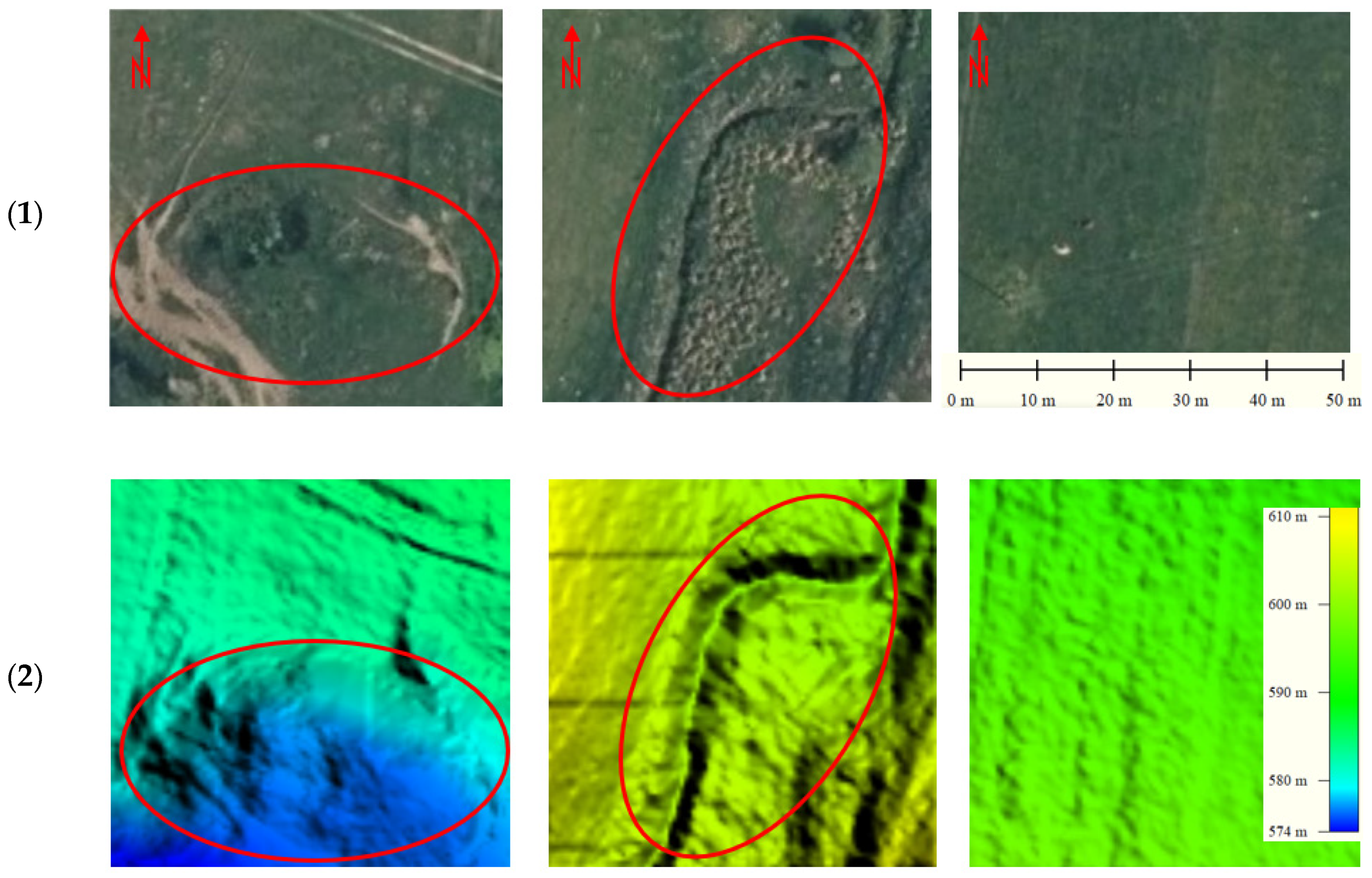
In the passability analysis, three parts of the terrain were used. On two of them, there were microrelief objects that we can visually identify from the orthophotomap or DEM visualization, which are likely to be identified as impassable areas. The third part is a flat terrain, which is a passable terrain from a military point of view, as there are no height differences and other terrain obstacles. This was used to check whether the script works correctly. The test areas of interest were squares measuring 50 m by 50 m, and they are located in the south part of Poland near Tylicz city—49°24′N, 21°01′E (Figure 1). The test areas are shown in Figure 2, where the characteristic microrelief shapes are marked. These terrain objects can potentially hinder the movement of vehicles.

2.2. Geomatics Data Used in the Experimentation

In the conducted research, two sources of data were used. The first was light detection and ranging (LIDAR) data that were obtained from the Head Office of Geodesy and Cartography from National Geodesy and Cartography Resource (denoted later in the article as LIDAR). This is a repository of all analogue and digital materials concerning geodesy and cartography that are used in different fields, such as the national economy, national defence, science, and culture [40]. These data are available for the whole of Poland’s territory. Their incontrovertible advantage is the ease in acquisition. We can download a part of LIDAR data for any area located in Poland with use of a web browser. The downloaded data are distributed as text files that contain coordinates (X, Y, Z) of points disposed evenly as a net with spacing of 0.5 m for urban areas (standard II) or 1 m for other areas (standard I). The data were interpolated from the point cloud acquired from the airborne laser scanning (LIDAR). A model with the resolution of 0.5 by 0.5 m was available for all three test areas.
The main principles of LIDAR technology are described in [41,42]. LIDAR data are binary files containing point clouds in LAS (Laser) format, which is designed for the processing of LIDAR point cloud data. The accuracy of the DEM created from this source can reach about 0.03 m (paved surface), 0.1 m (natural surface without vegetation), 0.2 m (surface covered with vegetation), and 0.5 m (very thick vegetation) [43]. According to the official data distributor, the mean squared error of the elevations used for research is within 0.2 m [40].
The second source of used data was the unmanned aerial vehicles photogrammetry data (denoted later as UAV). The use of UAVs allowed us to obtain the low altitude images and also photogrammetry data of the chosen terrain [44]. This data can be used, for example, for generating high resolution DEMs and 3D models of different objects or the point cloud data. The DEMs used in this research were generated from the point cloud data obtained from the aero triangulation process. The data was classified and filtered first. The accuracy of the obtained models was close to the accuracy of the LIDAR data [45] because, from the point cloud, we are able to obtain elevation models with horizontal accuracy of 0.05 m and vertical accuracy of 0.1 m as was shown, e.g., in [46]. Obtaining image data using UAV photogrammetry methods, apart from the obvious advantages (low cost, speed, and accuracy of the obtained data), depends to a large extent on the weather conditions [47,48].
The source data for this research were acquired in February in 2019 year with use of a Trimble UX-5 HP airframe, which was equipped with a Sony a7R camera with a 36.64 mm of focal length. The flying platform was equipped with a dual-frequency GPS receiver recording data with 10 Hz frequency. The camera settings were defined in the manual mode, and the focus of the lens was set to infinity. The flight was executed at a 150 m altitude in the east-west direction, assuming that endlap and sidelap were symmetrical and totalled 75%.
Endlap is the longitudinal overlap (along the direction of flight line) and sidelap is the transversal overlap (see [49,50]). This allowed us to obtain a ground sampling distance (GSD) of 0.02 m. This produced JPEG images, which were processed in Inpho UASMaster software. On the area of interest, there were 10 signalled ground control points (GCP) that were designed and measured and four independent check points (CP). All points were measured with use of real time kinematic (RTK) technique in a global navigation satellite system (GNSS). The terrain coordinates of the GCPs were determined with mean errors totalling: mx = 0.04 m, my = 0.04 m, and mz = 0.08 m, whereas in the CPs there were the following mean errors: mx = 0.04 m, my = 0.05 m, and mz = 0.09 m. The σ0 error for the whole block was 7.2 μm/1.5 px. As far as the exterior orientation is concerned, their mean standard deviation of translations and rotations are presented in the Table 1.
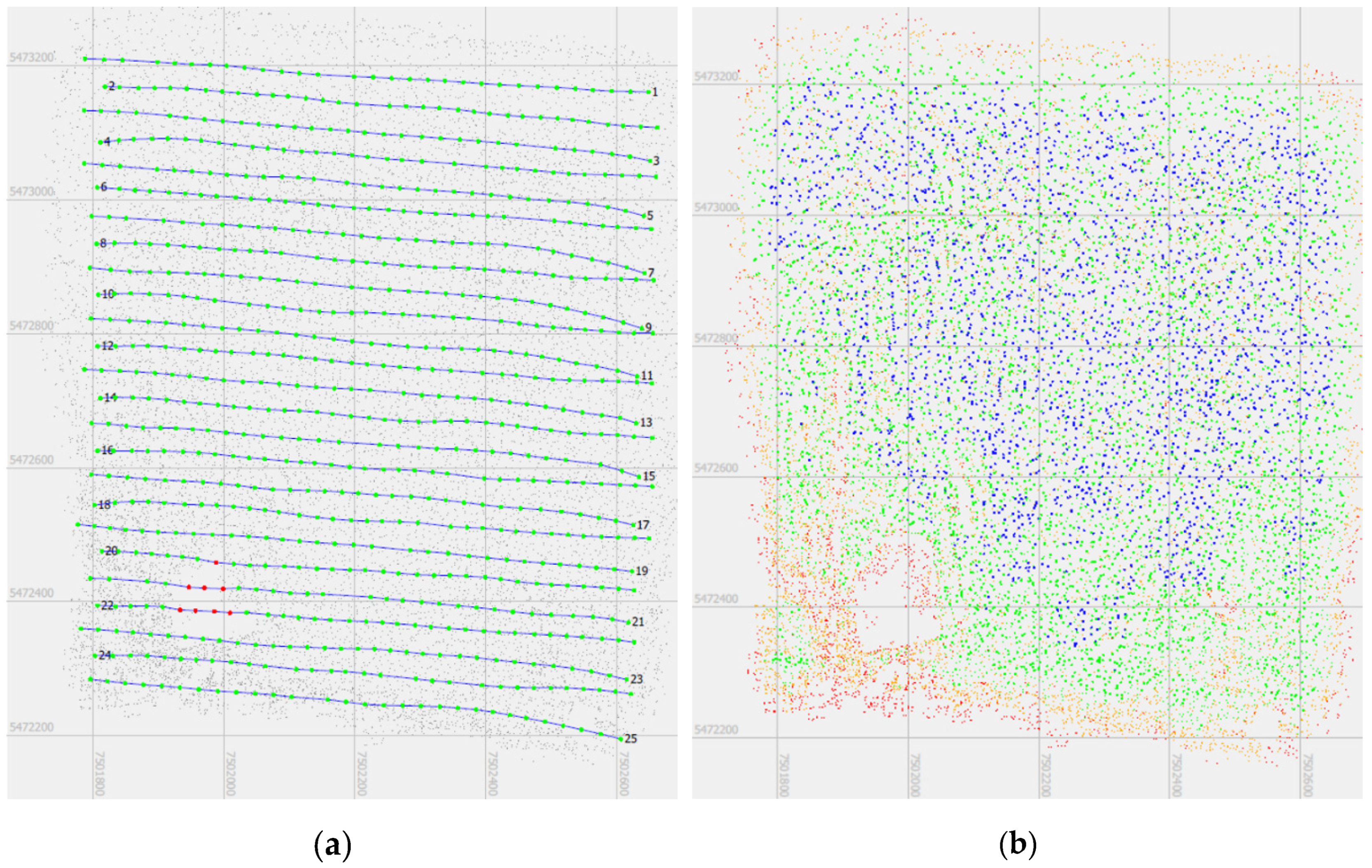
The resulting accuracy of the obtained point cloud was for horizontal coordinates (X, Y) of 0.06–0.07 m and for the vertical coordinate (Z) of 0.1 m. The flight path and the tie points distribution are presented in the Figure A1 in Appendix A.

3. Method

3.1. Preparing and Processing Data

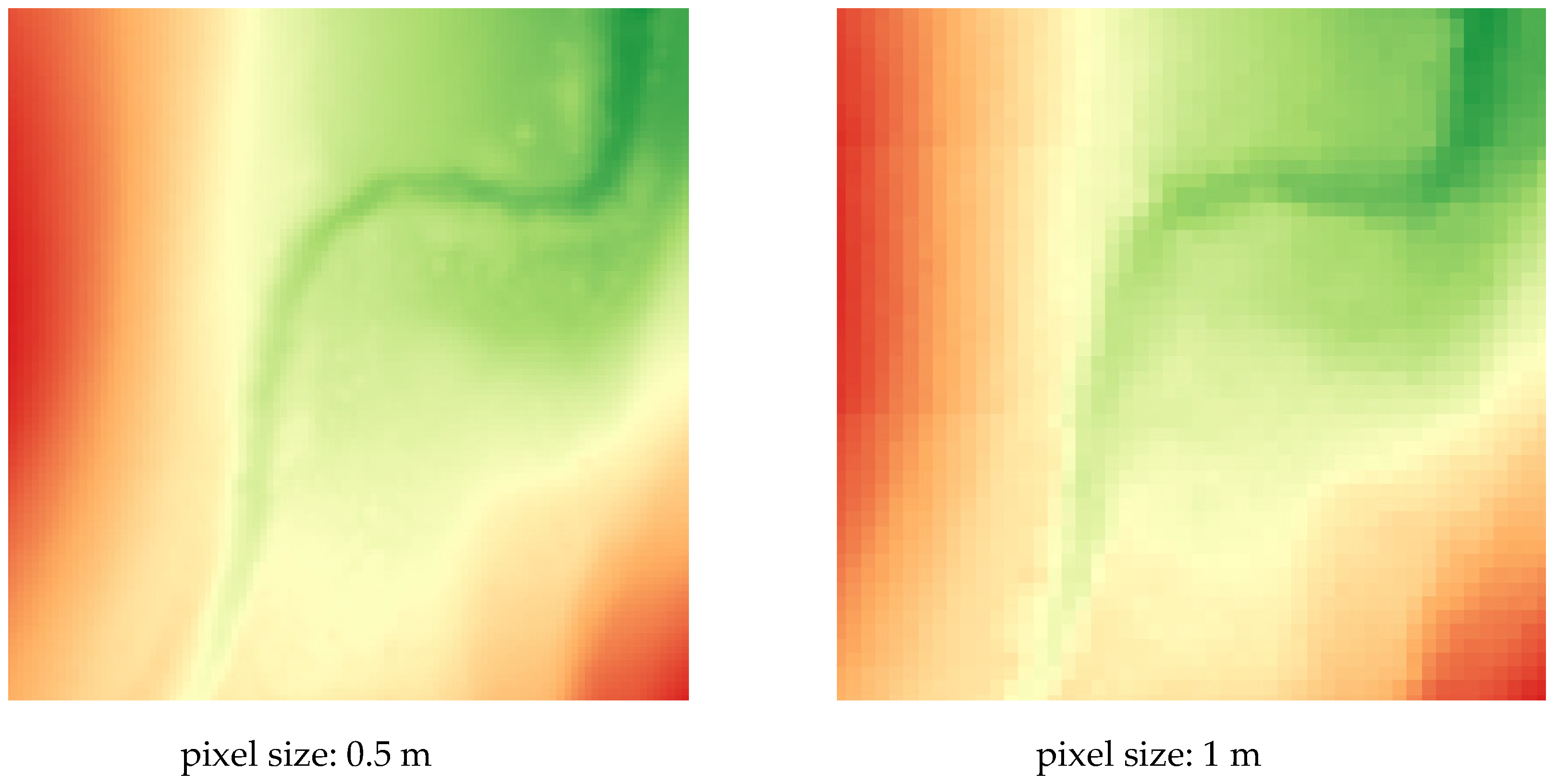
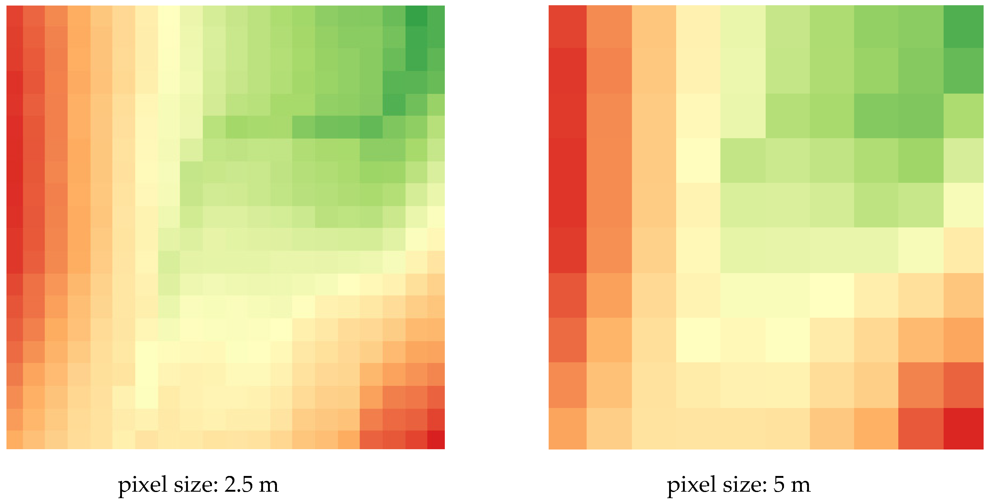
To determine the influence of the pixel size of the used DEMs on the accuracy of the obtained passability maps, analyses were conducted on different resolution DEMs. They were created from two sources of data: LIDAR and the UAV photogrammetry data in four different resolutions (0.5, 1, 2.5, and 5 m). Their visualizations are presented in Figure 3. The aim of the differentiation of pixel sizes was to calculate the processing time of the script, which allowed us to determine the dependence between the running time of the tool and the detail of the model. The increase in the DEM pixel size therefore allowed us to reduce the generation time of the passability map and, consequently, to develop it on a larger area in a shorter time.
The microrelief shapes are characterized by the small size; thus, to capture them, the research was conducted on a high-resolution DEM. We can assume that the pixel size of the model should not be greater than 5 m, because smaller microrelief objects that could be an obstacle to a vehicle would not be identified. From the LIDAR point cloud, we are able to produce models with a 0.5 m pixel size and vertical accuracy to 0.2 m; therefore, the use of this kind of data is legitimate [40].
To summarize, we acquired two points clouds from different sources, and the following step is to create digital elevation models from the classified points. To do so, we interpolated point data to obtain the pixel value of the DEM. The whole process was conducted in ArcGIS software. In the used tool “LAS Dataset to Raster” there were two types of interpolation:
  • Binning—The determination of the pixel value relies on examining the points that fall within the defined pixel. The final value can be chosen as the minimum, maximum, or average of the points [51].
  • Triangulation—To determine the final value, the Delaunay triangulation was used. This creates a surface made from a network of triangles and then rasterizes it.
The binning method is mainly used for high-density data, when we are sure that, in each pixel, there will be at least one point [52]. For the digital elevation model, the best setting is to use the minimum value, because the algorithm chooses then the lowest point (bare ground) inside the pixel [53]. However, triangulation is used with low-density data, because the pixel value is determined by the surface of the triangles. To see the difference between these two interpolation methods, a comparison was conducted. The two DEMs used the same parameters; however, different interpolation methods were subtracted. The obtained results are presented in Table 2.
As we can see in Table 2, the differences between the two types of interpolations were not high, and, due to the high density of the data, the binning method was chosen.

3.2. Terrain Passability Analysis Assumptions

The determination of the terrain passability was conducted for three vehicles used in the Polish Armed Forces: Honker, Star 266, and HMMWV (High Mobility Multipurpose Wheeled Vehicle; colloquially: Humvee). Their appearance is presented in Figure 4.
A Honker is a Polish off-road passenger vehicle, a Star 266 is an off-road truck designed to transport cargo or people on roads and off-roads, whereas a Humvee is a four-wheel drive armoured vehicle that is used in military operations for multiple purposes (from medical to combat). There are certain crucial tactical and technical parameters that influence the cross-country movement of each of the vehicles the most, which will be used in the presented methodology. They are listed in Table 3.
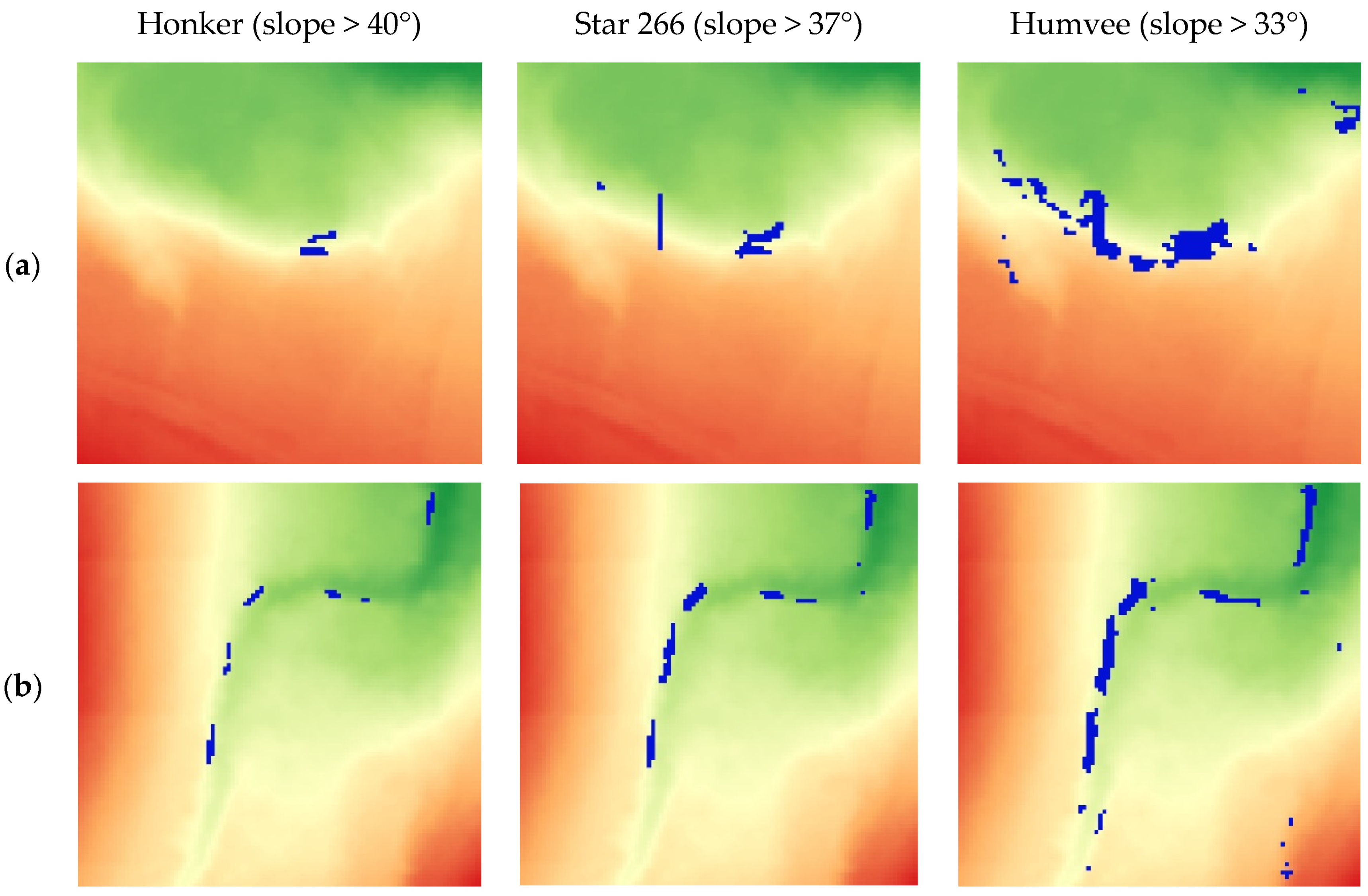
The passability analysis was divided into two parts. The first part was conducted in QGIS software, where the slope map was created and then the change of slope was calculated. The computed values were compared with the approach and descent angles to identify impassable areas. The impassable areas due to the slope angle are presented in Figure 5. For the analysis, we took the lowest value from both approach and descent angles to include all possible directions of movement.
As shown in [36], this method does not detect places where the vehicle can hit the ground with the area of the chassis between the wheels. Thus, to solve this problem, a tool in the Python programming environment was developed. The main working principle of this script was to calculate the chassis plane equation and check if, at a given point, the height of the terrain is greater than the height of the chassis. When such a case occurred, the analyzed point was classified as impassable. The input elevation data was the DEM in ASCII XYZ Grid format. This is a text file that stores the coordinates (X, Y, Z) of regularly spaced points. The size of the grid is dependent on the resolution of the elevation model. The research was conducted iteratively individually for each point of the grid. We assumed that the currently analyzed point of the model is a centroid of the chassis. The script only considered the section of the chassis between wheels what we can see in Figure 6.
Simplistically, the developed algorithm can be characterized as an iterative situating the vehicle model in each point of the elevation model of the analyzed terrain (assuming tangency of its tires with the ground). If, as a result of this positioning, the terrain crosses the chassis, it is assumed that the analyzed part of the terrain is classified as impassable. The research was conducted for different directions of vehicle movement (different angles of vehicle rotation towards the terrain). The developed methodology can be used for different kinds of vehicles. We simply need to know the vehicles’ parameters, as listed in Table 3 (then, we are able to change these parameters in the script).

3.3. The Principle of Working of the Developed Algorithm

The procedure to determine whether the chassis hits the ground was based on the assumptions of coordinate geometry in three-dimensional space. The movement of a vehicle is considered in four main directions: south–north, east–west, north-east–south-west, and north-west–south-east, and so there are four scripts, which differ in the disposition of the vehicle. It does not matter if the vehicle is moving, for instance, northward or southward because the procedure considers only the wheelbase, track width, and ground clearance (without front and rear overhang, which are typically different) and, thus, may be considered as one case. The working principle of the procedure will be shown on the basis of the south–north direction case. The steps of the process are listed below:
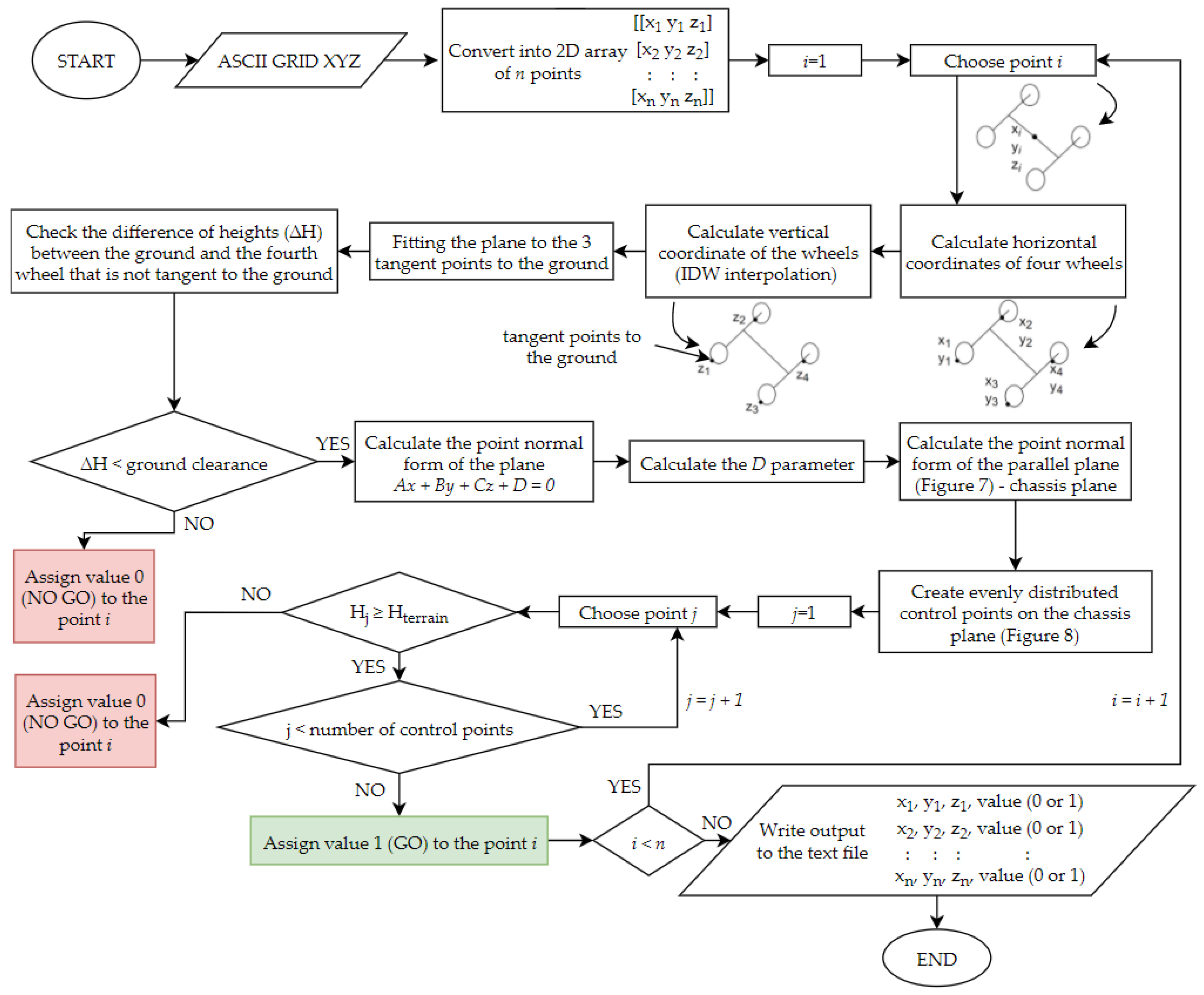
  • The elevation model in ASCII XYZ Grid format is converted into a two-dimensional array with three columns (X, Y, Z) and a number of rows equal to the number of points in the model. The script is, thereby, able to perform the mathematical operations on the data.
  • The procedure from this point iterates through each point of the model (row in the array). The coordinates of selected points are assigned to the centroid of the chassis. On the basis of the wheelbase and track width there are calculated horizontal coordinates of the four wheels. The computation considers the local slope of the terrain because, when the vehicle is pitched, the horizontal dimensions must be reduced.
  • In the next step, the z-coordinates of wheels are calculated. The script chooses four points of the grid that are closest to the wheel and then computes the height with the use of an inverse distance weighted (IDW) interpolation [58]. We can see this step in Figure 7.
  • Having calculated the coordinates of the wheels, the script computes the equation of the plane containing three tire contact points with the ground. At the beginning, four plane equations are calculated (containing three out of four tangent points in different configurations), and then the procedure searches in which plane position the fourth point of the vehicle (which does not belong to the plane) has the least difference of heights with the theoretical point with the same horizontal coordinates that belongs to the plane. After this test, the best fitted plane is chosen for further analysis. If the difference of heights is greater than the ground clearance, the analyzed point of the elevation model is assigned the value 0, which indicates that this point is impassable. The finding of the plane equation comes to the determination of four parameters of the point normal form of the plane (1):
    Ax + By + Cz + D = 0,
    where A, B, C, and D are the parameters. The first three are calculated from the cross product of vectors created between two pairs of analyzed points, The D parameter is computed by the substitution of the coordinates of one analyzed point into formula (2).
    D = −(Ax + By + Cz),
    where x, y, and z are the coordinates of one of the tangent points.
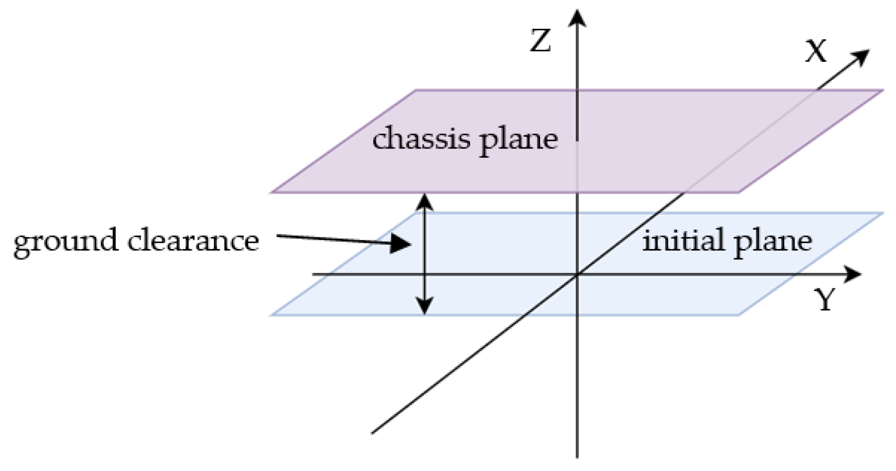
  • The aim of the next step is to compute the plane that approximates the chassis plane. To do that, we must calculate the parallel plane to the one that has already been determined. The value of the shift (distance between two planes) is equal to the ground clearance. This situation is shown in Figure 8.
  • This step extracts the part of the chassis plane that is limited by the wheels. Then, inside the resulting rectangle, the algorithm creates evenly distributed control points. It divides the distances between the wheels (wheelbase and track width) into even segments and places control points between them. As a result, we obtain a grid of points located in the chassis plane, which we can see in Figure 9. The distances between the points depend on the vehicle and especially on their parameters. The algorithm divides the wheelbase and track width values in each vehicle into four even parts.
  • Finally, the script checks each control point for whether its height exceeds the height of the terrain interpolated from the model. Unless all points meet this requirement (are higher than points on terrain), the analyzed point of the model is assigned the value 0 (impassable).
  • At the end of the process, the script creates a text file with coordinates of each point and an appended value of the passability (NO GO terrain—0 and GO terrain—1). On the basis of this file, we can distinguish the impassable terrain and calculate the statistics, which are presented further in the later section.
For the better visualization of the whole process, a block diagram was created. This shows the detailed process that the ASCII GRID XYZ file must undergo to obtain the file with points of the model and the indicator of the passability. The diagram is presented in Figure 10.
The processing of the vehicle location for each point of the used DEM makes the whole process time consuming. Due to this, to speed up the execution of the script, multiprocessing was set. This indicates that the program evenly divides the whole sum of the elevation model points into several processes, and they are executed simultaneously. Performance tests were conducted on a computer with the following parameters:
  • Model: ASUS X556UAK
  • Processor: Intel® Core™ i5-7200U CPU @ 2.71 GHz
  • Operating system: Windows 10 ×64 operating system
  • RAM: 20 GB
The obtained execution times of the script on a computer with the above parameters are listed further in the later section. Based on the combination of the analysis results and performance tests, we were able to select the most optimized settings for the whole passability analysis process. This means that we could select the number of processes and the pixel size of the model to obtain the best solution in the fastest way. The results of the tests are described in the next section.

4. Results

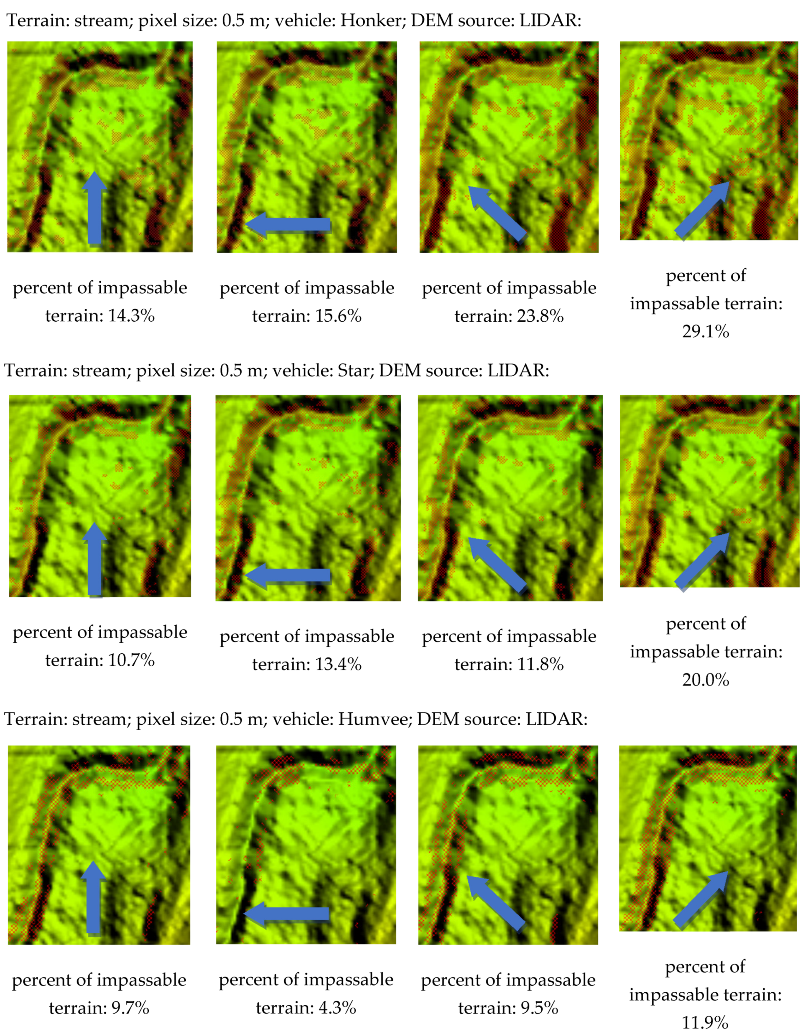
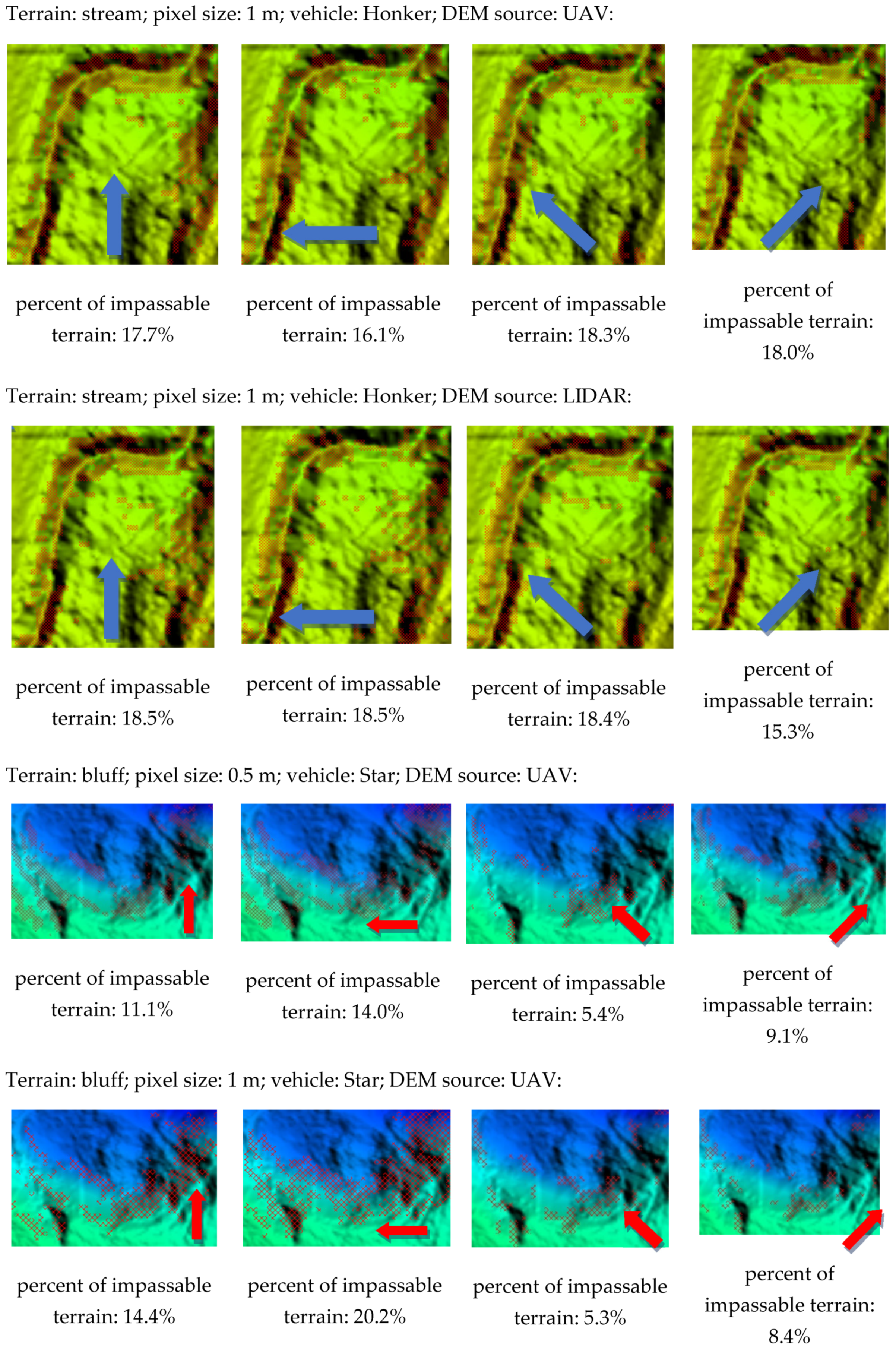
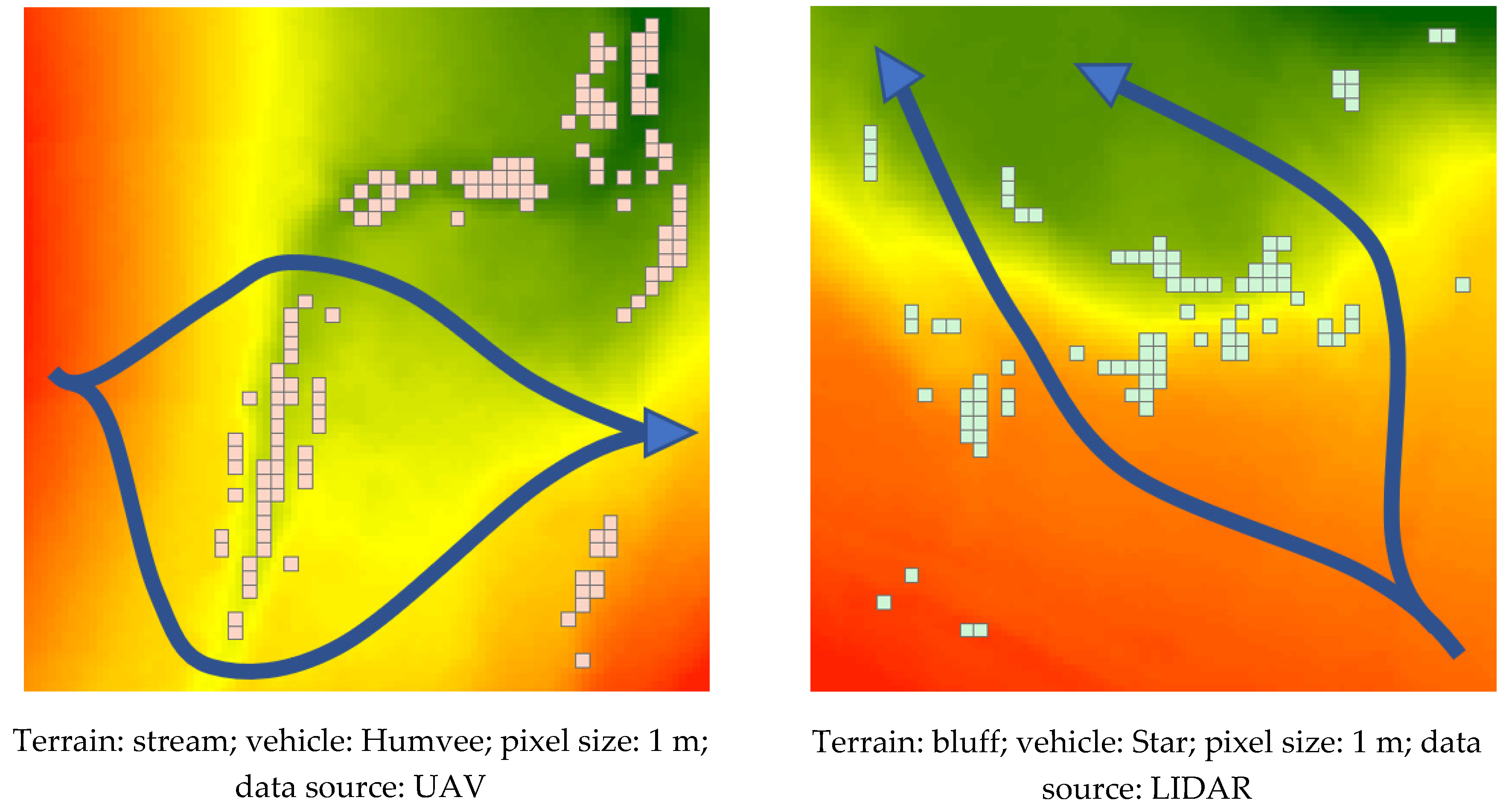
The products of the analysis show the impassable parts of the tested terrains in multiple configurations for each vehicle. The results are computed for each direction of movement (north, east, northeast, and northwest), for two kinds of data (from LIDAR and from UAV) and for each resolution of DEM (0.5, 1, 2.5, and 5 m). Due to the large number of results, some of them are only presented briefly (Figure 11). The arrow indicates the direction of the vehicle movement.
As far as the flat terrain is concerned (Figure 2c), due to the expectations, there was no impassable terrain indicated by the algorithm. This shows that the script works correctly.
The execution times of the script are also crucial factors of the analysis. They depend mainly on the pixel size of the model. The higher the resolution of the model is, the more time it will take to complete the execution of the script. The results of the performance analysis for tested areas (50 × 50 m) are listed in Table 4.

5. Discussion

To analyze the differences between the generated DEMs, in the first step, their statistics have been calculated. These are DEMs for each kind of analyzed terrain (bluff, stream, and flat) and generated on the basis of the LIDAR and UAV data that were described in Section 2. Their statistics are presented in Table 5. We can conclude from them that the differences between models from disparate sources were not high. They did not exceed 1 m value in any case. At this point, we are not able to determine which source of data is more credible. This will be verified in future research by taking field measurements.
The change of the pixel size did not strongly influence the average height. There were no differences between the 0.5 and 1 m resolution models, and between the 1, 2.5, and 5 m, there was 20 cm maximally. As far as the standard deviation is concerned, its value depends on the kind of terrain, which the elevation model represents. The highest value was in the bluff terrain and the lowest was the flat terrain. In the second step of the comparison, visualizations of differences between models obtained using two sources of data were generated (the results are presented in Figure 12).
The obtained visualizations confirm the results presented in Table 5. The maximal differences between models did not exceed 0.8 m. However, the spatial distribution of disparities showed that the biggest deviations were on the areas of high height differences, which can have an impact on the results of the conducted passability analysis.
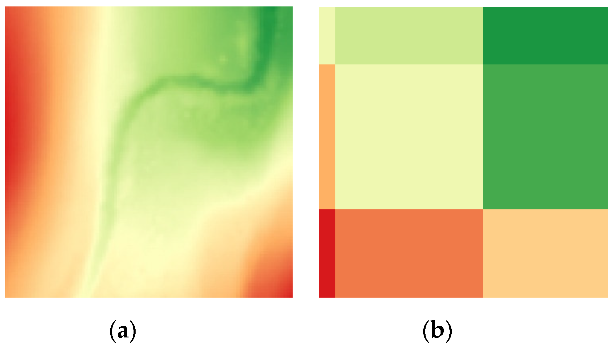
To make a tool that detects the microrelief objects on the digital elevation model), an accurate model must be used. There are some DEMs acquired in Poland and used widely in Polish Armed Forces and in the NATO countries: LIDAR (light detection and ranging) data, DTED (digital terrain elevation data), SRTM (shuttle radar topographic mission), and UAV (unmanned aerial vehicle) photogrammetry data. As far as the DTED and SRTM data are concerned, their horizontal accuracy is about 30 m, and the vertical accuracy is about 20 m. The pixel size of these models is about ten times larger than the size of vehicles; thus, it is worth showing that the use of these models in microrelief object detection and presented passability analysis is limited due to their relatively high resolution in comparison with the LIDAR and UAV data. This is shown in Figure 13.
The obtained results show that, in most cases, when the pixel size increased, the amount of impassable terrain indicated by the algorithm grew. There were also certain exceptions from that rule, especially when the analysis concerned the northwest and northeast direction. In this configuration, the percent of impassable terrain in the model with the 1 m pixel size was smaller than the percent in the model with the 0.5 m pixel size. This is shown on the charts in Figure 14.
From the charts (Figure 14), we can also conclude that the size of impassable terrain decreased proportionally to the increase in the ground clearance value of each vehicle. This behaviour of the results proclaims that the algorithm calculates correctly. As far as the results from the model with the 2.5 and 5 m pixel size are concerned, in most cases, there was a rapid growth of the impassable areas. Assuming that the results from the 0.5 m pixel size model are the most accurate, we can conclude that the outputs from the 2.5 and 5 m models are too generalized. This indicates that there is too much impassable terrain indicated in comparison with the results from the more accurate models. The 3D visualization of the obtained results allows us to see the described dependences (Figure 15).
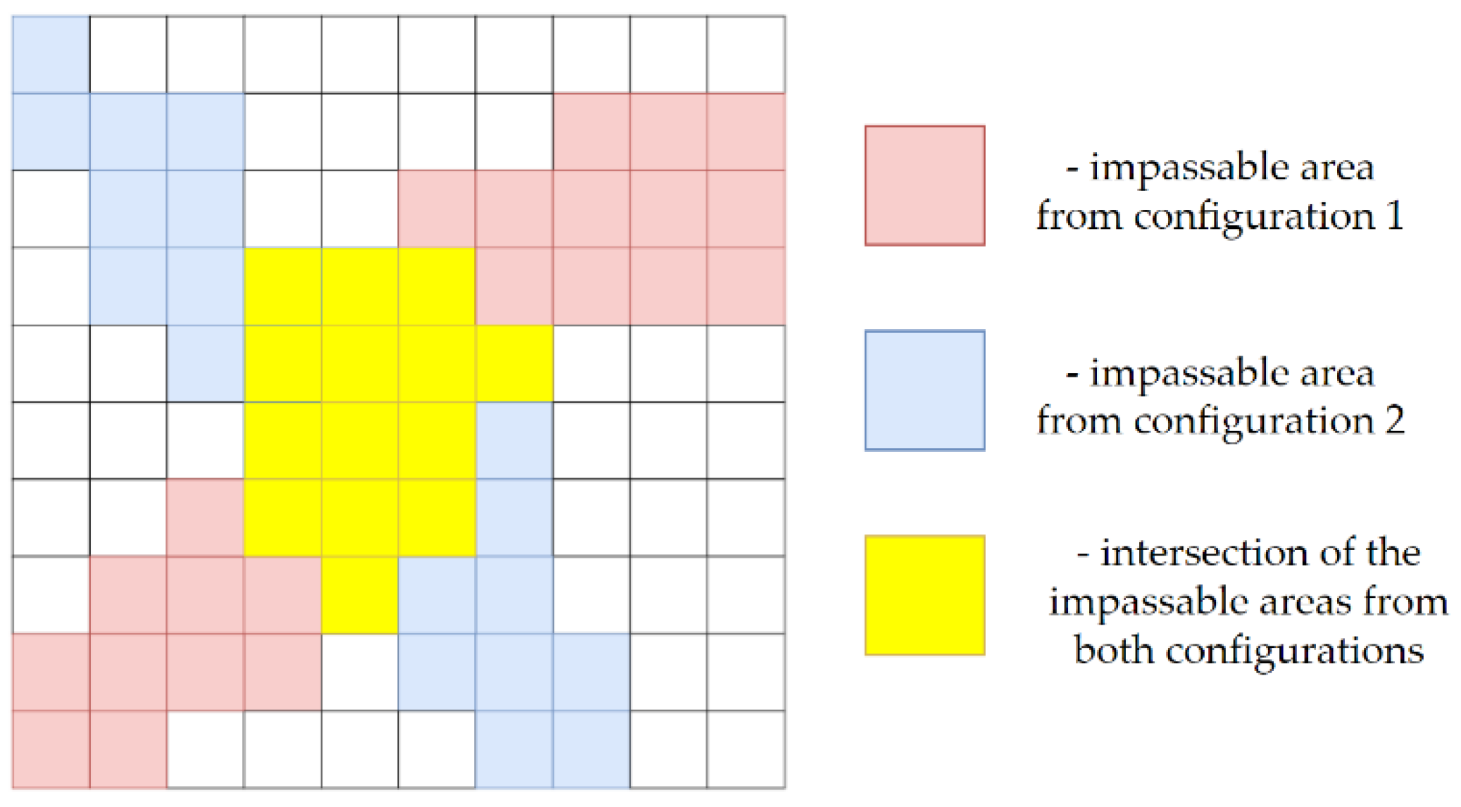
When the amount of the impassable terrain e.g., in two cases is the same, this does not mean that the equivalent terrain was indicated as NO GO. To check the consistency of the obtained results, an intersection analysis was conducted. The outcomes are the values of intersection between each configuration of results (from different resolution models and from different source of the data) and the values of the size of non-common impassable areas. The design of this analysis is presented in Figure 16.
Due to the large number of outputs, the discussion will concern only the results for the Honker vehicle moving northward. The values of the intersection are presented in Table 6, Table 7, Table 8, Table 9, Table 10 and Table 11, as explained in Figure 17.
From the results presented in the above tables, we can conclude that, in most cases, there was a distinct advantage of common impassable area over uncommon terrain for the compared models. However, in some cases, e.g., in Table 9, in comparison of two 0.5 m models, we can see that the intersection value is the same or smaller than the uncommon area. All differences between common and uncommon parts of the impassable terrain may result from the fact that DEMs from UAV and LIDAR are not the same as was presented in Table 2. Despite such numerical differences, the visualization of the impassable areas shows that the character of the indicated areas is similar, as is shown in Figure 18. We present examples with different parameter configurations.
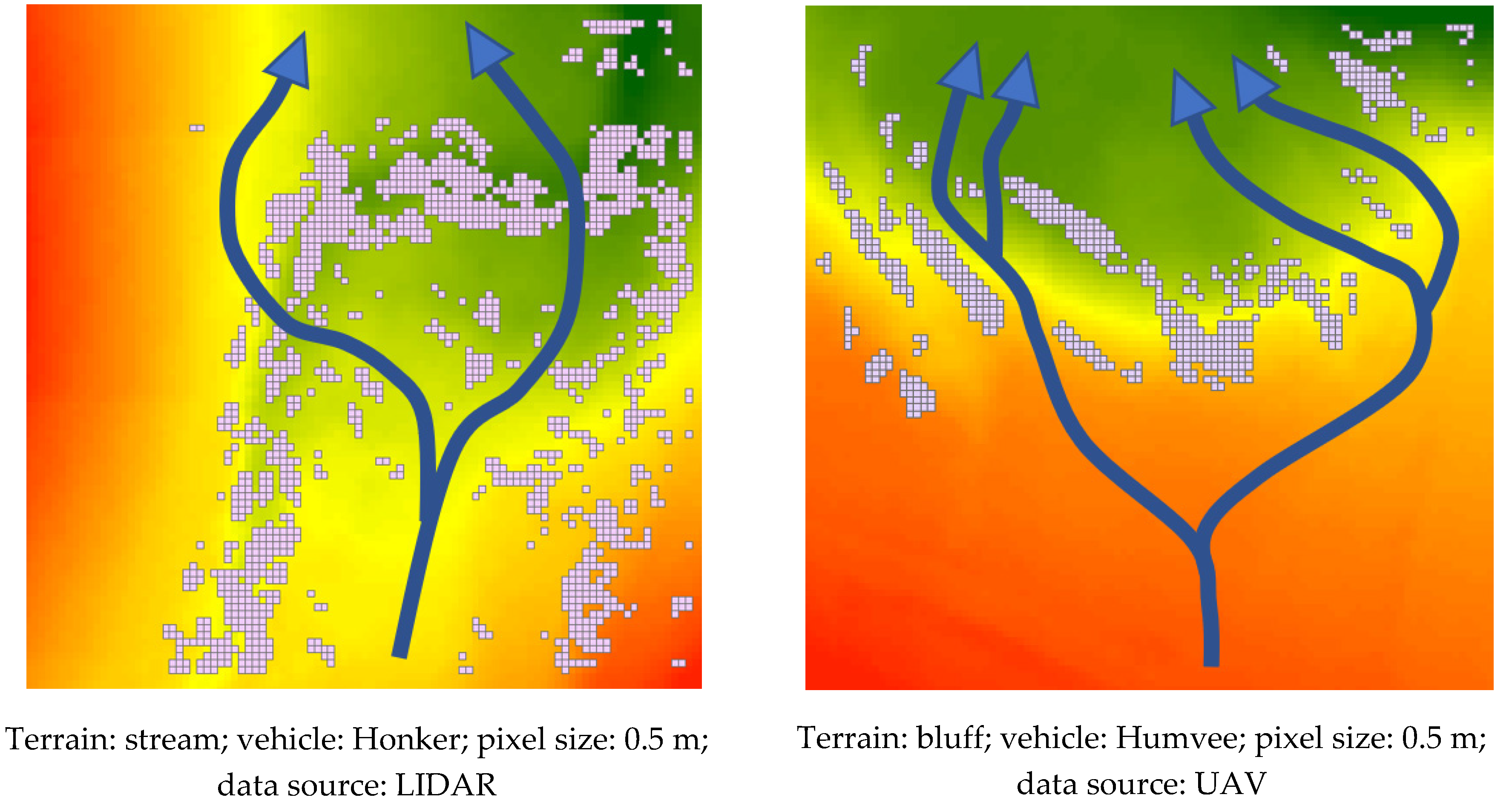
This conclusion is important from the point of view of the operational use of maps, because, while planning a route through a given terrain, the driver is only interested in the possibility of overcoming it. The structure and exact shape of the impassable area is not crucial information. However, detailed elevation models allow the finding of narrow, passable corridors, which eventually allow the overcoming of terrain by performing maneuvers to avoid obstacles. Examples are presented in Figure 19. Arrows indicate the possible routes of vehicles and their widths represent the real vehicle widths.
The next question is, which output is better: the results from LIDAR or UAV data? To define the word “better” in this question, we have to find an unambiguous coefficient that will show the superiority of the obtained results. A good solution for this problem is to use the indices described in the spatial autocorrelation theory. On the basis of the spatial distribution of objects, the autocorrelation analysis measures whether and to what extent they influence each other.
The best coefficients of spatial autocorrelation are Geary’s and Moran’s indices [59]. Both are used for the same data context and, in most applications, give very similar results. However, they differ in the scale and the meaning of the output value. Geary’s index takes only positive values from 0 to 2 (0—objects are clustered, 1—objects are distributed randomly and independently, and 2—objects are dispersed) while Moran’s indices are values from −1 and 1 and they are much more intuitive (1—objects are clustered, 0—objects are distributed randomly and independently, and −1—objects are dispersed) [59]. For this reason, in the spatial autocorrelation analysis, we used Moran’s coefficient.
In the comparison of the obtained passability areas, the results from the UAV data were perceived as more consistent and clustered than the LIDAR output. In the first example in Figure 18, the passability terrains of the following parameters: terrain, stream, pixel size, 0.5 m, and vehicle: Honker are visualized. We can clearly see that there are more separate parts from LIDAR data than from UAV. Such dependencies are visible in each pair of compared results. The confirmation of these observations are the values of Moran’s coefficients. They are listed in Table 12.
As anticipated, we can see that, as far as the lower resolutions are concerned (0.5 and 1 m), the values are highly positive, and there is a slight advantage of UAV over LIDAR data. In greater resolutions (2.5 and 5 m), the coefficients are the same and almost equal to the maximum value of the index. This indicates that the 0.5 and 1 m outputs were highly clustered; however, the results from the UAV data were slightly more clustered. Taking the 2.5 and 5 m values into consideration, their almost maximum Moran indexes show that the impassable areas were almost fully clustered. The reason for these very high results could be the small area of the analyzed terrain, where there was not enough space for any distribution of impassable areas.
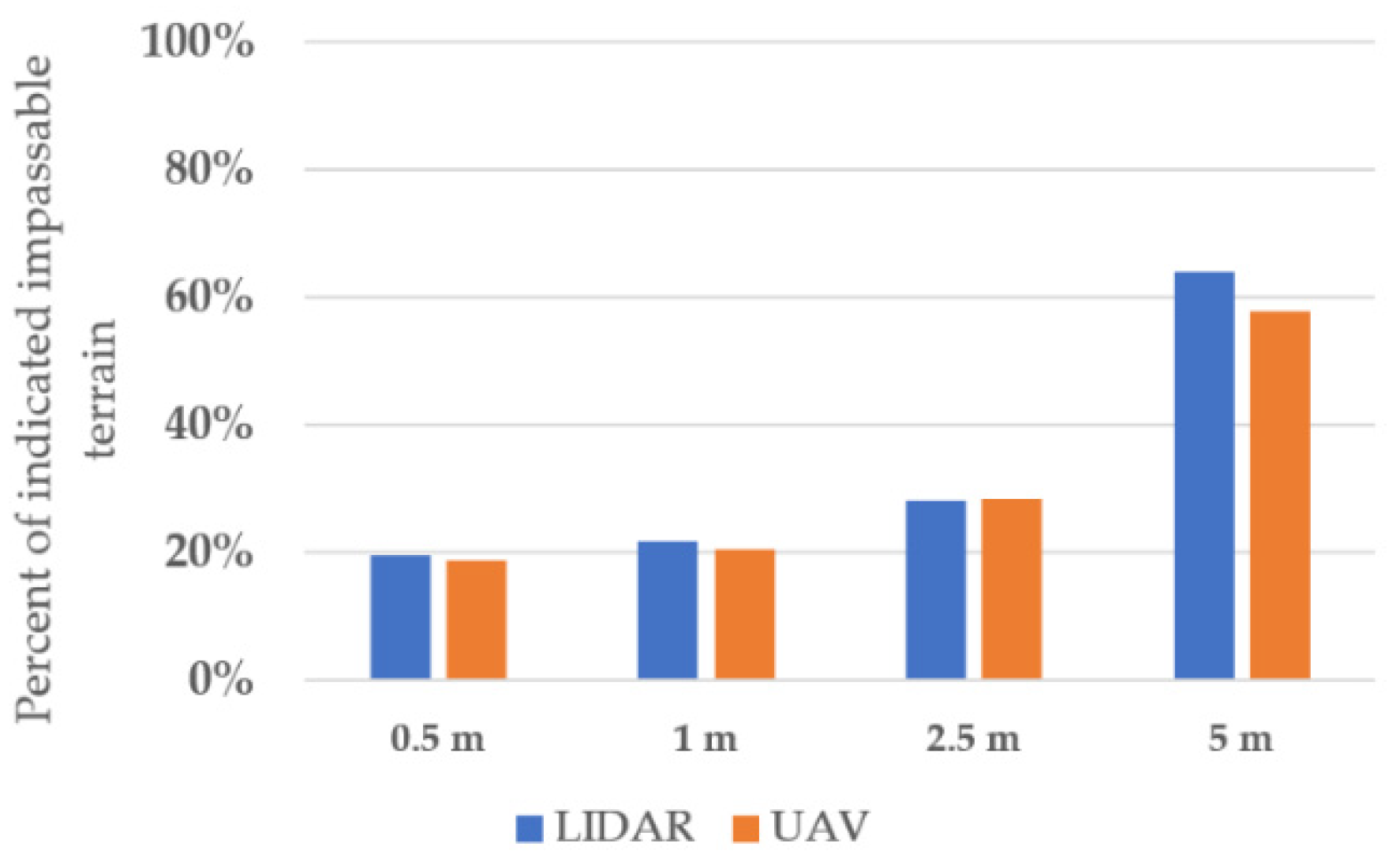
The results showed that, in most cases, when the analysis was based on the models of the same parameters but different data sources, the percentages of impassable terrain indicated by the script were similar. The biggest variances were in the 5 m pixel size models. This was mainly caused by the inaccuracy of the model in detecting the microrelief shapes and the large area that was covered by one pixel in this model (25 m2—1% of the whole analyzed terrain). Considering that LIDAR data can be easily obtained from the state geodetic and cartography and the creation of the model from the UAV is much more complex and time consuming, the more optimal solution is to create DEMs for the passability analysis from the LIDAR data. The chart showing dependences between the percent of indicated impassable terrain (Honker vehicle, bluff terrain, 0.5 m pixel size) from elevation models from different data sources is presented in Figure 20.
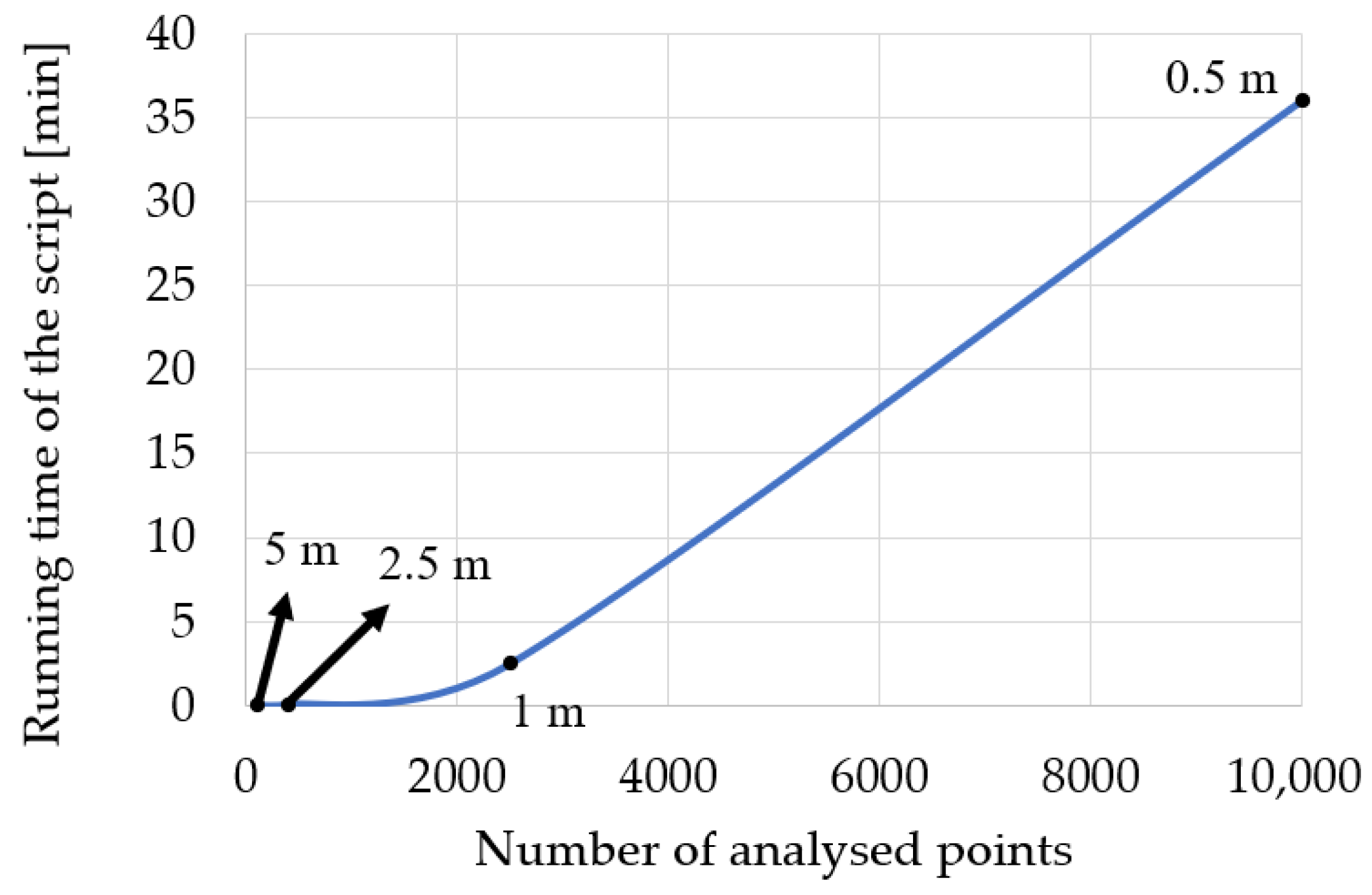
In Figure 21, we can see the dependence between the time of the execution of the script and the number of analyzed points. The chart was created based on Table 4. The number of analyzed points grew due to decrease in the pixel size of the elevation model. We can see from the presented chart that the increase in the points caused an exponential growth of the running time of the script. The analyzed terrain was relatively small (50 × 50 m). If the passability analysis concerned larger terrain, the whole process would last much longer. To choose the most optimal option, we must consider two main factors: the accuracy of the results and the time of obtaining them. The conclusions are described in the next section.
There are also some limitations in the developed method. One of them is that the algorithm does not take the resilience of shock absorbers into consideration. This is a factor that can hardly be predicted and algorithmized due to the multiples of other factors conditioning the behaviour of shock absorbers, e.g., quality of roads (on which the vehicle moves), the driver’s style of driving, or the working conditions. This method cannot be used for tanks or other vehicles that have tracks, because the wheelbase in this case is unidentifiable, and consequently we can hardly predict in which place of the ground the tracks are tangent. The presented methodology also does not take soil parameters into account.

6. Conclusions

The conducted research demonstrated clearly that the presented methodology with the implemented authorial method of the parallel shift of the plane was able to detect microrelief objects and, consequently, impassable areas with different resolution digital elevation models. In the analysis, we used DEMs created on the basis of LIDAR and UAV photogrammetry data in different resolutions: 0.5, 1, 2.5, and 5 m as well as the parameters of three kinds of vehicles widely applicable in the Polish Armed Forces: Honker, Star, and Humvee. The differentiation of resolutions was made to answer the question: which model is the most efficient in obtaining the best results possible in the shortest time?
The obtained results show, as expected, that the amount of the impassable area depends on the ground clearance of the vehicle. If this value grows, the number of impassable cells decreases. We can see this dependence in Figure 14. This behaviour demonstrates the correctness of the developed methodology. In different resolution outcomes, in most cases, there was a rapid growth of impassable areas between the 1 and 2.5 m pixel sizes. This proves that the output from the mentioned models is too generalized in comparison with the smaller resolution models, which are considered to be more accurate. However, the results from the 2.5 m and 5 m models should not be rejected, because they have use in the analysis conducted at the higher operational level of command. Smaller resolutions (0.5 and 1 m) show more detailed characteristics of impassable areas.
An important factor that influences the evaluation is also the intersection area, which shows the degree of consistency between the obtained outputs. In Table 6, Table 7, Table 8, Table 9, Table 10 and Table 11, we present the numerical values of intersection. We can conclude from these that the correspondence grew with the increase in the pixel size of the used models. In smaller resolutions, the proportions between the common and uncommon impassable areas fluctuated around 50%. Despite such unsatisfactory numerical values, the visualization of outcomes showed a high consistency between them. We can see in Figure 18 that, in most corresponding cases, there was a distinguishable main character of impassable area. The difference between outputs was mainly caused by the disparity of the used DEMs.
As far as the source of the data is concerned, the results from UAV photogrammetry data visually appeared to be less dispersed, what indicates the higher quality of the data. The confirmation of this convincement is the Moran index, which provides the numerical value of the spatial autocorrelation between results. The more clustered the objects are, the higher the value of the index is. The coefficients at smaller resolutions (0.5 and 1 m) were higher for the models from the UAV data, and, at higher resolutions (2.5 and 5 m), they were the same.
This proves that DEMs created from the UAV photogrammetry data were qualitatively better. However, Figure 20 presents the dependences between the number of impassable areas in the corresponding models. This shows that, in most cases, there is more or less the same quantity of impassable area in the range of the model of the same parameters but with different data sources. The LIDAR data can be easily acquired from the State Geodetic and Cartography and UAV data must be obtained from the photogrammetry record and the aero triangulation process. This makes the UAV data more difficult and time consuming to acquire.
Taking the above into consideration, both data sources should be treated in a complementary manner. On terrain where there are available LIDAR data, which can be acquired from the governmental sources, their use provides the desired results. The unquestionable advantage of these data is the ease of obtaining them, making all works related with the preparation of passability maps possible to perform as office work.
They are available almost for the whole Poland’s territory, and, consequently, detailed passability maps can be developed for a huge area. On the other hand, military or crisis management operations can be realized on areas where there is no access to such high-resolution data. Then, the acquisition of image data with use of UAVs and their development to obtain detailed DEMs can be indispensable. The time of the DEM obtaining a base of photogrammetry data can be progressively shortened due to the ongoing automation of the image processing process.
An important factor is also the time of the analysis. The dependence between the time and pixel size is presented in Figure 21. We can see the exponential growth of the time when increasing the pixel size and, consequently, the number of analyzed pixels. The most rapid rise of the time is noticeable between the 1 and 0.5 m models. All analyses in this research were conducted on relatively small areas (50 × 50 m). When it comes to larger terrains, the processing times could increase rapidly. The optimalization of the script will be studied in further research. All conducted tests allowed us to determine the most optimal solution for the passability analysis. To obtain accurate results in the optimal time, the best option was to use the 1 m model from the UAV photogrammetry data. This resolution is slightly less accurate than the 0.5 m; however, the time of the analysis is considerably higher.
Finally, the conducted analyses showed that the developed tool, which examines the terrain in terms of the passability, can be used in different aspects of the terrain analysis process. As was already mentioned, the higher resolution models (2.5 and 5 m) can be used at the operational level in planning military operations. On the other hand, 0.5 and 1 m, due to their high accuracy, may be used and implemented in unmanned ground vehicles. The knowledge of obstacles located in the terrain will increase the effectiveness of actions taken by the UGV. In this article, the issue of verification of the data was not raised and will be examined in further research.

Author Contributions

Conceptualization: W.D. and K.P.; methodology: W.D. and K.P.; software: W.D.; validation: W.D. and K.P.; formal analysis: W.D.; investigation: W.D.; resources: W.D.; data curation: W.D.; writing—original draft preparation: W.D.; writing—review and editing: K.P.; visualization: W.D.; supervision: K.P.; project administration: K.P.; funding acquisition: K.P. All authors have read and agreed to the published version of the manuscript.

Funding

This research was funded by Military University of Technology in Warsaw, Faculty of Civil Engineering and Geodesy, Institute of Geospatial Engineering and Geodesy statutory research funds No. 793/2020.

Acknowledgments

LIDAR data were obtained from the Head Office of Geodesy and Cartography.

Conflicts of Interest

The authors declare no conflict of interest.

Appendix A

Figure A1. (a) Flight path. (b) Tie points distribution; PL-2000 coordinate system (EPSG: 2178).
Remotesensing 12 04146 g0a1

References

  1. Ministry of National Defence. Defence Standard NO-06-A015:2012, Terrain—Rules of Classification—Terrain Analysis on Operational Level; Ministry of National Defence of Poland: Krakow, Poland, 2012.
  2. Department of the Army. Army Field Manual No. 5–33: Terrain Analysis; Headquarters Department of the Army: Washington, DC, USA, 1990. Available online: http://everyspec.com/ARMY/FM-Field-Manual/FM_5-33_13620/ (accessed on 30 October 2020).
  3. Balzter, H.; Cole, B.; Thiel, C.; Schmullius, C. Mapping CORINE land cover from Sentinel-1A SAR and SRTM digital elevation model data using random forests. Remote Sens. 2015, 7, 14876–14898. [Google Scholar] [CrossRef] [Green Version]
  4. Pennock, D.J.; Zebarth, B.J.; De Jong, E. Landform classification and soil distribution in hummocky terrain, Saskatchewan, Canada. Geoderma 1987, 40, 297–315. [Google Scholar] [CrossRef]
  5. Bielecka, E.; Jenerowicz, A.; Pokonieczny, K.; Borkowska, S. Land cover changes and flows in the Polish Baltic coastal zone: A qualitative and quantitative approach. Remote Sens. 2020, 12, 2088. [Google Scholar] [CrossRef]
  6. Pašakarnis, G.; Maliene, V. Towards sustainable rural development in Central and Eastern Europe: Applying land consolidation. Land Use Policy 2010, 27, 545–549. [Google Scholar] [CrossRef]
  7. Mościcka, A.; Pokonieczny, K.; Wilbik, A.; Wabiński, J. Transport accessibility of Warsaw: A case study. Sustainability 2019, 11, 5536. [Google Scholar] [CrossRef] [Green Version]
  8. Hošková-Mayerová, Š. Geospatial data reliability, their use in crisis situations. Int. Conf. Knowl. Based Organ. 2015, 21, 694–698. [Google Scholar] [CrossRef] [Green Version]
  9. Hubacek, M.; Ceplova, L.; Brenova, M.; Mikita, T.; Zerzan, P. Analysis of vehicle movement possibilities in terrain covered by vegetation. In Proceedings of the 2015 International Conference on Military Technologies (ICMT), Brno, Czech Republic, 19–21 May 2015; pp. 1–5. [Google Scholar] [CrossRef]
  10. Rybansky, M. Determination the ability of military vehicles to override vegetation. J. Terramech. 2020, 91, 129–138. [Google Scholar] [CrossRef]
  11. Rybansky, M. Modelling of the optimal vehicle route in terrain in emergency situations using GIS data. In 8th International Symposium of the Digital Earth; IOP Publishing Ltd.: Bristol, UK, 2014; Volume 18, p. 012131. [Google Scholar]
  12. Hubáček, M.; Rybansky, M.; Cibulova, K.; Brenov, M.; Ceplova, L. Mapping the passability of soils for vehicle movement. KVÜÕA Toim. 2016, 21, 5–18. [Google Scholar]
  13. Rybansky, M. Soil trafficability analysis. In Proceedings of the International Conference on Military Technologies (ICMT) 2015, Brno, Czech Repubic, 19–21 May 2015; pp. 1–5. [Google Scholar] [CrossRef]
  14. Hubáček, M.; Almášiová, L.; Dejmal, K.; Mertová, E. Combining different data types for evaluation of the soils passability. In The Rise of Big Spatial Data; Ivan, I., Singleton, A., Horák, J., Inspektor, T., Eds.; Springer International Publishing: Cham, Switzerland, 2017; pp. 69–84. [Google Scholar]
  15. Jayakumar, P.; Mechergui, D.; Wasfy, T.M. Understanding the effects of soil characteristics on mobility. In Proceedings of the 2017 International Design Engineering, Technical Conferences & Computers and Information in Engineering Conference, Cleveland, OH, USA, 6–9 August 2017. [Google Scholar] [CrossRef]
  16. McCullough, M.; Jayakumar, P.; Dasch, J.; Gorsich, D. The next generation NATO reference mobility model development. J. Terramech. 2017, 73, 49–60. [Google Scholar] [CrossRef]
  17. Bradbury, M.; Dasch, J.; Gonzalez, R.; Hodges, H.; Jain, A.; Iagnemma, K.; Letherwood, M.; McCullough, M.; Priddy, J. Next-Generation NATO Reference Mobility Model (NRMM) Development; Dasch, J., Jaykumar, P., Eds.; NATO: Bruxelles, Belgium, 2018. [Google Scholar]
  18. González, R.; Jayakumar, P.; Iagnemma, K. Stochastic mobility prediction of ground vehicles over large spatial regions: A geostatistical approach. Auton. Robot. 2017, 41, 311–331. [Google Scholar] [CrossRef]
  19. Gonzalez, R.; Jayakumar, P.; Iagnemma, K. An efficient method for increasing the accuracy of mobility maps for ground vehicles. J. Terramech. 2016, 68, 23–35. [Google Scholar] [CrossRef]
  20. Lessem, A.; Mason, G.; Ahlvin, R. Stochastic vehicle mobility forecasts using the nato reference mobility model. J. Terramech. 1996, 33, 273–280. [Google Scholar] [CrossRef]
  21. Maclaurin, B. Comparing the NRMM (VCI), MMP and VLCI traction models. J. Terramech. 2007, 44, 43–51. [Google Scholar] [CrossRef]
  22. Hofmann, A.; Hošková-Mayerová, Š.; Talhofer, V.; Kovařík, V. Creation of models for calculation of coefficients of terrain passability. Qual. Quant. 2014, 49, 1679–1691. [Google Scholar] [CrossRef]
  23. Rybansky, M.; Hofmann, A.; Hubacek, M.; Kovarik, V.; Talhofer, V. Modelling of cross-country transport in raster format. Environ. Earth Sci. 2015, 74, 7049–7058. [Google Scholar] [CrossRef] [Green Version]
  24. Pokonieczny, K.; Borkowska, S. Using high resolution spatial data to develop military maps of passability. In Proceedings of the 2019 International Conference on Military Technologies (ICMT), Brno, Czech Republic, 30–31 May 2019; pp. 1–8. [Google Scholar]
  25. Pokonieczny, K.; Mościcka, A. The influence of the shape and size of the cell on developing military passability maps. ISPRS Int. J. Geo Inf. 2018, 7, 261. [Google Scholar] [CrossRef] [Green Version]
  26. Pokonieczny, K. Automatic military passability map generation system. In Proceedings of the 2017 International Conference on Military Technologies (ICMT), Brno, Czech Republic, 31 May–2 June 2017; pp. 285–292. [Google Scholar]
  27. Pokonieczny, K. Use of a multilayer perceptron to automate terrain assessment for the needs of the armed forces. ISPRS Int. J. Geo Inf. 2018, 7, 430. [Google Scholar] [CrossRef] [Green Version]
  28. Rybansky, M. Effect of the Geographic Factors on the Cross Country Movement during Military Operations and the Natural Disasters; Rerucha, V., Ed.; University of Defence Brno: Brno, Czech Republic, 2007; ISBN 978-80-7231-238-2. [Google Scholar]
  29. Talhofer, V.; Hošková-Mayerová, Š.; Hofmann, A. Improvement of digital geographic data quality. Int. J. Prod. Res. 2012, 50, 4846–4859. [Google Scholar] [CrossRef]
  30. Richmond, P.W.; Mason, G.L.; Coutermarsh, B.A.; Pusey, J.; Moore, V.D. Mobility Performance Algorithms for Small Unmanned Ground Vehicles; Engineer Research and Development Center, Geotechnical and Structures Laboratory: Vicksburg, MS, USA, 2009. [Google Scholar]
  31. Shoop, S.; Knuth, M.; Wieder, W. Measuring vehicle impacts on snow roads. J. Terramech. 2013, 50, 63–71. [Google Scholar] [CrossRef]
  32. Ropero, F.; Muñoz, P.; R-Moreno, M.D. TERRA: A path planning algorithm for cooperative UGV–UAV exploration. Eng. Appl. Artif. Intell. 2019, 78, 260–272. [Google Scholar] [CrossRef]
  33. Hubacek, M.; Kovarik, V.; Kratochvil, V. Analysis of influence of terrain relief roughness on DEM accuracy generated from Lidar in the Czech Republic territory. ISPRS Int. Arch. Photogramm. Remote Sens. Spat. Inf. Sci. 2016, XLI-B4, 25–30. [Google Scholar] [CrossRef]
  34. Szombara, S.; Lewińska, P.; Żądło, A.; Róg, M.; Maciuk, K. Analyses of the Prądnik riverbed shape based on archival and contemporary data sets—Old maps, LiDAR, DTMs, orthophotomaps and cross-sectional profile measurements. Remote Sens. 2020, 12, 2208. [Google Scholar] [CrossRef]
  35. Wierzbicki, D. Multi-camera imaging system for UAV photogrammetry. Sensors 2018, 18, 2433. [Google Scholar] [CrossRef] [PubMed] [Green Version]
  36. Dohnal, F.; Hubacek, M.; Sturcova, M.; Bures, M.; Simkova, K. Identification of microrelief shapes along the line objects over DEM data and assessing their impact on the vehicle movement. In Proceedings of the 2017 International Conference on Military Technologies (ICMT), Brno, Czech Republic, 31 May–2 June 2017; pp. 262–267. [Google Scholar] [CrossRef]
  37. Dohnal, F.; Hubacek, M.; Simkova, K. Detection of microrelief objects to impede the movement of vehicles in terrain. ISPRS Int. J. Geo Inf. 2019, 8, 101. [Google Scholar] [CrossRef] [Green Version]
  38. Fryskowska, A.; Wróblewski, P. Mobile laser scanning accuracy assessment for the purpose of base-map updating. Geod. Cartogr. 2018, 67, 35–55. [Google Scholar] [CrossRef]
  39. Stereńczak, K.; Ciesielski, M.; Balazy, R.; Zawiła-Niedźwiecki, T. Comparison of various algorithms for DTM interpolation from LIDAR data in dense mountain forests. Eur. J. Remote Sens. 2016, 49, 599–621. [Google Scholar] [CrossRef]
  40. Head Office of Geodesy and Cartography. GUGiK Data PZGiK. Available online: http://www.gugik.gov.pl/pzgik (accessed on 21 October 2020).
  41. Starek, M.J. Light detection and ranging (LIDAR). In Encyclopedia of Estuaries; Encyclopedia of Earth Sciences Series; Springer: Dordrecht, The Netherlands, 2016; Volume 383. [Google Scholar] [CrossRef]
  42. Elprocus. LIDAR System (Light Detection and Ranging) Working and Applications; Elprocus: Hyderabad, India, 2019. [Google Scholar]
  43. ISOK. IT System for Country Protection Against Extreme Hazards (ISOK). Available online: https://isok.gov.pl/ (accessed on 30 October 2020).
  44. Lalak, M.; Wierzbicki, D.; Kędzierski, M. Methodology of processing single-strip blocks of imagery with reduction and optimization number of ground control points in UAV photogrammetry. Remote Sens. 2020, 12, 3336. [Google Scholar] [CrossRef]
  45. Sammartano, G.; Spanò, A. DEM generation based on UAV photogrammetry data in critical areas. In Proceedings of the 2nd International Conference on Geographical Information Systems Theory, Applications and Management, Rome, Italy, 26–27 April 2016; pp. 92–98. [Google Scholar] [CrossRef]
  46. Ajayi, O.G.; Salubi, A.A.; Angbas, A.F.; Odigure, M.G. Generation of accurate digital elevation models from UAV acquired low percentage overlapping images. Int. J. Remote Sens. 2017, 38, 3113–3134. [Google Scholar] [CrossRef]
  47. Sekrecka, A.; Wierzbicki, D.; Kedzierski, M. Influence of the sun position and platform orientation on the quality of imagery obtained from unmanned aerial vehicles. Remote Sens. 2020, 12, 1040. [Google Scholar] [CrossRef] [Green Version]
  48. Kedzierski, M.; Wierzbicki, D.; Sekrecka, A.; Fryskowska, A.; Walczykowski, P.; Siewert, J. Influence of lower atmosphere on the radiometric quality of unmanned aerial vehicle imagery. Remote Sens. 2019, 11, 1214. [Google Scholar] [CrossRef] [Green Version]
  49. Pepe, M.; Fregonese, L.; Scaioni, M. Planning airborne photogrammetry and remote-sensing missions with modern platforms and sensors. Eur. J. Remote Sens. 2018, 51, 412–436. [Google Scholar] [CrossRef]
  50. Roch, J.L. UAV classification and associated mission planning. In Multi-Rotor Platform-Based UAV Systems; ISTE: London, UK, 2020; pp. 27–44. ISBN 978-1-78548-251-9. [Google Scholar]
  51. LAS Dataset to Raster Function—Help ArcGIS for Desktop. Available online: https://desktop.arcgis.com/en/arcmap/10.3/manage-data/raster-and-images/las-dataset-to-raster-function.htm (accessed on 26 October 2020).
  52. LAS to Raster Function—Help ArcGIS for Desktop. Available online: https://desktop.arcgis.com/en/arcmap/10.3/manage-data/raster-and-images/las-to-raster-function.htm (accessed on 26 October 2020).
  53. Creating Raster DEMs and DSMs from Large Lidar Point Collections—Help ArcGIS Desktop. Available online: https://desktop.arcgis.com/en/arcmap/10.3/manage-data/las-dataset/lidar-solutions-creating-raster-dems-and-dsms-from-large-lidar-point-collections.htm (accessed on 26 October 2020).
  54. Wikipedia.pl. Honker; Wikipedia, the Free Encyclopaedia. Available online: https://pl.wikipedia.org/wiki/Honker (accessed on 20 October 2020).
  55. Brach, J. Star 266—Modernization. Available online: http://www.magnum-x.pl/artykul/star-266-projekty-modernizacji-czesc-ii (accessed on 20 October 2020).
  56. Military.com. High Mobility Multipurpose Wheeled Vehicle (HMMWV). Available online: https://www.military.com/equipment/high-mobility-multipurpose-wheeled-vehicle-hmmwv (accessed on 20 October 2020).
  57. Tyminski, Z. Vehicle 4x4 Honker 2000—User Manual 2008. Available online: http://honkerteam.pl/wp-content/uploads/2016/04/Instrukcja-Obs%C5%82ugi-HONKER-wrzesien-2008.pdf (accessed on 20 October 2020).
  58. Achilleos, G.A. The inverse distance weighted interpolation method and error propagation mechanism—Creating a DEM from an analogue topographical map. J. Spat. Sci. 2011, 56, 283–304. [Google Scholar] [CrossRef]
  59. Curran, P. Spatial autocorrelation. Appl. Geogr. 1989, 9, 138–139. [Google Scholar] [CrossRef]
Figure 1. The location of the analyzed parts of the terrain.
Remotesensing 12 04146 g001
Figure 2. Three kinds of terrain with their 3D visualization and marked microrelief objects on them: (a) convex object (bluff); (b) concave object (stream); (c) flat terrain; (1) orthophotomap; (2) digital elevation model (DEM) visualization; (3) 3D DEM visualization.
Remotesensing 12 04146 g002aRemotesensing 12 04146 g002b
Figure 3. Used DEMs with different pixel sizes on examples of concave terrain.
Remotesensing 12 04146 g003aRemotesensing 12 04146 g003b
Figure 4. Analyzed vehicles: (a) Honker [54]; (b) Star 266 [55]; and (c) HMMWV (High Mobility Multipurpose Wheeled Vehicle; colloquially: Humvee) [56].
Remotesensing 12 04146 g004
Figure 5. DEMs with indicated impassable areas due to the slope angle: (a) bluff terrain, and (b) stream terrain.
Remotesensing 12 04146 g005
Figure 6. Visualized parameters of the vehicle: (a) side view (1—checked by the change of slope; 2—checked by the Python script); and (b) rear view.
Remotesensing 12 04146 g006
Figure 7. The conception of the inverse distance weighted (IDW) interpolation.
Remotesensing 12 04146 g007
Figure 8. The parallel shift of the plane.
Remotesensing 12 04146 g008
Figure 9. Evenly distributed control points in the analyzed part of the chassis plane (bird’s eye view).
Remotesensing 12 04146 g009
Figure 10. Block diagram of the process.
Remotesensing 12 04146 g010
Figure 11. Results of the analysis.
Remotesensing 12 04146 g011aRemotesensing 12 04146 g011bRemotesensing 12 04146 g011c
Figure 12. Visualization of the differences.
Remotesensing 12 04146 g012
Figure 13. The comparison between high- and low-resolution elevation data: (a) LIDAR data (0.5 m pixel size); (b) digital terrain elevation data (DTED) 2 data (30 m pixel size).
Remotesensing 12 04146 g013
Figure 14. Percent of impassable areas indicated by the script.
Remotesensing 12 04146 g014
Figure 15. 3D visualization of the bluff terrain with indicated impassable areas depending on the pixel size.
Remotesensing 12 04146 g015
Figure 16. Illustrative figure of the intersection analysis.
Remotesensing 12 04146 g016
Figure 17. Interpretation of the record of results.
Remotesensing 12 04146 g017
Figure 18. Impassable areas and the indicated main characteristics.
Remotesensing 12 04146 g018aRemotesensing 12 04146 g018b
Figure 19. Movement corridors that avoid impassable areas.
Remotesensing 12 04146 g019aRemotesensing 12 04146 g019b
Figure 20. Comparison of the percent of impassable terrain (Honker vehicle, bluff terrain, 0.5 m pixel size) from elevation models from different data sources.
Remotesensing 12 04146 g020
Figure 21. Dependence between the running time of the script and the number of analyzed points (pixel size near dots).
Remotesensing 12 04146 g021
Table 1. Mean standard deviations of translations and rotations.
TranslationsX (m)Y (m)Z (m)Total (m)
0.090.070.110.16
RotationsOmega (°/1000)Phi (°/1000)Kappa (°/1000)
0.0240.0330.072
Table 2. Statistics of the differences between two types of interpolation.
SourceKind of TerrainPixel Size [m]Minimum [m]Maximum [m]Average [m]Standard Deviation
light detection and ranging (LIDAR)bluff0.5−0.360.400.000.04
1−0.520.570.000.06
2.5−0.750.580.000.09
5−0.721.210.010.18
stream0.5−0.470.390.000.05
1−0.460.350.000.06
2.5−0.370.280.000.07
5−0.360.410.010.11
flat0.5−0.100.110.000.02
1−0.080.080.000.02
2.5−0.100.090.000.03
5−0.100.080.000.03
unmanned aerial vehicle (UAV)bluff0.5−0.280.190.000.02
1−0.560.120.000.03
2.5−0.490.180.000.05
5−0.190.310.020.09
stream0.5−0.140.170.000.02
1−0.190.270.000.03
2.5−0.350.410.000.07
5−0.310.700.030.16
flat0.5−0.070.060.000.01
1−0.060.060.000.01
2.5−0.090.070.000.02
5−0.060.060.000.02
Table 3. Parameters of the analyzed vehicles [55,56,57].
VehicleWheelbase (m)Track Width (m)Ground Clearance (m)Approach Angle (°)Descent Angle (°)
Honker2.901.650.224040
Star 2662.992.000.333742.5
Humvee3.302.000.436333
Table 4. Times of the script execution.
Pixel Size (m)Number of Grid Points in the ModelExecution Time
0.510,00036 min
125002 min 30 s
2.54004 s
51001 s
Table 5. Statistics of the digital elevation models.
SourcePixel Size (m)Minimum (m)Maximum (m)Average (m)Standard Deviation
bluffLIDAR0.5574.23585.66580.743.15
1574.24585.62580.743.15
2.5574.48585.60580.893.12
5576.02585.53581.193.03
UAV0.5573.52585.02580.053.16
1573.54584.96580.053.16
2.5574.00584.98580.253.11
5575.22584.87580.453.05
streamLIDAR0.5598.19608.69603.592.27
1598.23608.62603.592.27
2.5598.70608.57603.812.28
5599.21608.48604.052.28
UAV0.5598.00608.41603.312.31
1598.11608.34603.312.31
2.5598.68608.38603.552.31
5598.96608.25603.772.32
flatLIDAR0.5592.51598.37595.341.36
1592.55598.34595.341.36
2.5592.74598.34595.461.37
5592.93598.28595.541.36
UAV0.5591.89597.62594.631.35
1591.92597.59594.631.35
2.5592.06597.57594.721.36
5592.25597.53594.811.36
Table 6. Intersection between impassable areas of the Honker moving northward in bluff terrain (UAV and LIDAR data).
Honker
Bluff
Direction: N
SourceUAV
Pixel Size0.5 m1 m2.5 m5 m
SourcePixel SizeImpassable Terrain (m2)447472644925
LIDAR0.5 m469 169 213 359 635
191278210259184285179290
1 m502 180 135 326 553
235267165337184318130372
2.5 m638 161 131 119 394
352286297341113525107531
5 m1025 142 99 138 25
720305652373214506125900
Table 7. Intersection between impassable areas of the Honker moving northward in bluff terrain (LIDAR data).
Honker
Bluff
Direction: N
SourceLIDAR
Pixel Size0.5 m1 m2.5 m5 m
SourcePixel SizeImpassable Terrain (m2)4695026381025
LIDAR0.5 m469 138
138331
1 m502 159 0
1923100502
2.5 m638 185 171 0
3542843073310638
5 m1025 157 118 107 0
71331264138449453101025
Table 8. Intersection between impassable areas of the Honker moving northward in bluff terrain (UAV data).
Honker
Bluff
Direction: N
SourceUAV
Pixel Size0.5 m1 m2.5 m5 m
SourcePixel SizeImpassable Terrain (m2)447472644925
UAV0.5 m447 0
0447
1 m472 150 0
1752970472
2.5 m644 157 136 0
3542903083360644
5 m925 156 109 144 0
6342915623634255000925
Table 9. Intersection between impassable areas of the Honker moving northward in stream terrain (UAV and LIDAR data).
Honker
Stream
Direction: N
SourceUAV
Pixel Size0.5 m1 m2.5 m5 m
SourcePixel SizeImpassable Terrain (m2)35040812251550
LIDAR0.5 m344 178 222 1021 1298
17217215818614020492252
1 m426 164 157 953 1219
24018617525115427295331
2.5 m1375 96 70 100 525
1121254103733825011253501025
5 m1525 89 76 275 75
12642611193332575950501475
Table 10. Intersection between impassable areas of the Honker moving northward in stream terrain (LIDAR data).
Honker
Stream
Direction: N
SourceLIDAR
Pixel Size0.5 m1 m2.5 m5 m
SourcePixel SizeImpassable Terrain (m2)34442613751525
LIDAR0.5 m344 0
0344
1 m426 132 0
2142120426
2.5 m1375 88 90 0
1119256103933601375
5 m1525 80 76 294 0
12612641173352444108101525
Table 11. Intersection between impassable areas of the Honker moving northward in stream terrain (UAV data).
Honker
Stream
Direction: N
SourceUAV
Pixel Size0.5 m1 m2.5 m5 m
SourcePixel SizeImpassable Terrain (m2)35040812251550
UAV0.5 m350 0
0350
1 m408 126 0
1842240408
2.5 m1225 150 141 0
102520095826701225
5 m1550 106 106 287 0
1306244124830261293801550
Table 12. Moran’s coefficients of the obtained results.
Pixel Size (m)BluffStream
LIDARUAVLIDARUAV
0.50.680.700.610.64
10.800.820.760.81
2.50.930.930.920.92
50.960.960.950.95
Publisher’s Note: MDPI stays neutral with regard to jurisdictional claims in published maps and institutional affiliations.