Article

Mapping Aboveground Woody Biomass on Abandoned Agricultural Land Based on Airborne Laser Scanning Data

1
Department of Forest Policy, Economics and Forest Management, National Forest Centre—Forest Research Institute Zvolen, T.G. Masaryka 22, 960 01 Zvolen, Slovakia
2
Department of Forest and Landscape Ecology, National Forest Centre—Forest Research Institute Zvolen, T.G. Masaryka 22, 960 01 Zvolen, Slovakia
3
Centre of Excellence of Forest-Based Industry, National Forest Centre—Forest Research Institute Zvolen, T.G. Masaryka 22, 960 01 Zvolen, Slovakia
*
Author to whom correspondence should be addressed.
Remote Sens. 2020, 12(24), 4189; https://doi.org/10.3390/rs12244189
Submission received: 23 November 2020 / Revised: 16 December 2020 / Accepted: 18 December 2020 / Published: 21 December 2020

Abstract

:
Mapping aboveground woody biomass (AGB) on abandoned agricultural land (AAL) is required by relevant stakeholders to monitor the spatial dynamics of farmland afforestation, to assess the carbon sequestration, and to set the appropriate management of natural resources. The objective of this study was, therefore, to present and assess a workflow consisting of (1) the spatial identification of AAL based on a combination of airborne laser scanning (ALS) data, cadastral data, and Land Parcel Identification System data, and (2) the prediction of AGB on AAL using an area-based approach and a nonparametric random forest (RF) model based on a combination of field and ALS data. Part of the second objective was also to evaluate the applicability of (1) the author-developed algorithm for the calculation of ALS metrics and (2) a single comprehensive RF model for the whole area of interest. The study was conducted in the forest management unit Vígľaš (Slovakia, Central Europe) covering a total area of 12,472 ha. Specifically, five reference areas consisting of 11,194 reference points were used to assess the accuracy of the spatial identification of AAL, and seventy-five ground reference plots were used for the development of the ALS-based AGB model and for assessing the accuracy of the AGB map. The overall accuracy of the spatial identification of AAL was found to be 93.00% (Cohen’s kappa = 0.82). The difference between ALS-predicted and ground-observed AGB reached a relative root mean square error (RMSE) at 26.1%, 33.1%, and 21.3% for the whole sample size, plots dominated by shrub species, and plots dominated by tree species, respectively.

Graphical Abstract

1. Introduction

Changes in the landscape related to the abandonment of agricultural land represent a problem in many regions of the world. This phenomenon is mainly notable in countries of Eastern and Central Europe, where the formerly intensively worked farmland has been abandoned due to deep social and political changes [1,2]. Moreover, the process of abandonment is intensified by the complicated ownership structure of land parcels (defragmentation), which leads to the loss of active management, especially in mountainous areas with less-productive soils. Here, the relevant drivers of agricultural land abandonment could also be the elevation, slope, erosion, clime, and fertility [3,4].
Uncontrolled cessation of agricultural production and the subsequent afforestation of agricultural land through forest succession, especially on land with good soil quality, is a serious challenge for effective natural resource management and environmental policy. Primarily, this phenomenon leads to the loss of agricultural land and has therefore had a tremendous impact on food security and local livelihoods [5]. Negative impacts on soil chemical composition due to higher carbon dioxide sequestration have also been identified [6]. Moreover, the restoration of abandoned agricultural land (AAL), already occupied by forest vegetation, is very difficult, time consuming, and expensive. On the other hand, in many environmental aspects, including biodiversity, the balance of positive and negative effects of land abandonment is still discussed [7].
Because of the causal effects related to the enormous scope of the present processes of land abandonment in many regions of the world, it is necessary to continuously monitor the aboveground woody biomass (AGB) on AAL and to include it in the global carbon storage and cycle [8]. However, ground-based monitoring is significantly limited for these purposes due to the fragmented occurrence and dynamics of land abandonment, especially in larger areas [9]. Remote sensing (RS) technologies represent a more effective way to acquire relevant information about AAL ecosystems. Specifically, airborne laser scanning (ALS) data provide an opportunity to complement ground-based monitoring [10]. This is primarily because ALS systems can penetrate a laser beam through even dense and multi-layered vegetation canopies to the ground, and ALS data can then be used to directly estimate a spatially explicit three-dimensional vegetation structure with submeter accuracy [11]. However, classification of the composition of tree species and nationwide AGB estimations using only ALS data has proven to be a difficult task. Therefore, airborne and/or spaceborne optical and/or radar data are often used for tree species classification [12,13] and to upscale local or regional estimations to the national level [14,15].
A comprehensive overview of RS-based applications focused on the spatial identification of AAL was published by [8]. According to this review, satellite platforms were identified as the most frequently used data source for AAL identification (e.g., Landsat, Terra Aqua, SPOT, Sentinel-2, Envisat-ASAR, RADARSAT-2, and Sentinel-1) [16,17]. Specifically, the majority of studies identified AAL using object-based image analysis with or without a fusion of machine learning algorithms [18,19] based on vegetation indexes, such as the normalized vegetation index (NDVI) [20,21]. Although ALS data were used less frequently as a primary data source [22,23], the combination of optical and/or radar data with ALS data was defined as a prospective solution for RS-based identification of AAL [8]. While many studies have examined the RS-based spatial identification of AAL, less attention has been paid to predicting AGB specifically in these areas. According to available studies, the relevant features extracted from high-resolution optical images of pixel or multi-pixel scale were mostly used for these purposes [24,25]. However, ALS [26] as well as a combination of other active and passive sensors (e.g., Landsat and PALSAR [27]) have been also investigated in AAL-specific ecosystems. For example, [28] assessed the performance of five vegetation indices, fractional green vegetation cover, and fractional coverage of vegetation in order to monitor shrub vegetation. [29,30,31] proposed to use an application of the crown volume index or NDVI in the case of woody vegetation.
Regardless of the source of RS data and the type of extracted features from this data, an area-based approach (ABA) is the most appropriate method for AGB estimation over large areas [32,33]. This is because ABA makes it possible to obtain model-unbiased estimates of AGB [34], and the requirements for RS data (e.g., point cloud density) or hardware are relatively low [32]. On the other hand, up-to-date ground data are still needed for preparing a model, and when tree-level information, such as stem number or species, is desired, ABA is less suitable [35]. In ABA, the response variable (e.g., AGB) is estimated through co-located metrics (e.g., height, intensity, and density). These metrics can be directly or indirectly computed from the RS data. Specialized software packages, such as FUSION (United States Forest Service, [36]) or LAStools (rapidlasso GmbH, [37]), are most commonly used for this purpose. However, the submodule “Point Cloud Metrics” implemented in the reFLex software (National Forest Centre, [38,39]) represents the newest alternative. This software includes only original sets of algorithms scripted in C# programming language and ALS metrics can be computed from first, last, or all returns considering the height thresholds defined by user. Regarding the development of final predictive models, the nonparametric machine learning techniques, such as random forest (RF), have the ability to identify complex relationships between predictor and response variables, therefore showing their superiority or promising level of performance over parametric methods for the estimation of AGB [40,41,42].
Many studies have used different RS data and modelling methods to predict AGB in forest, shrub, or grassland ecosystems (e.g., [10,32,33,34,35,38,39,40,41,42]). However, as far as we know, relatively few studies (e.g., [22,23,26]) have dealt with the spatial identification of AAL and prediction of AGB on AAL using ALS data. Moreover, an author-developed algorithm for the calculation of ALS metrics, which was used in this study, has not yet been broadly tested and reported. Therefore, the overall objective of this study was to present and asses a workflow consisting of (1) the spatial identification of AAL based on a combination of ALS data, cadastral data, and Land Parcel Identification System (LPIS) data, and (2) the prediction of AGB on AAL using ABA and a nonparametric RF model based on a combination of field and ALS data. Here, the applicability of (1) the author-developed algorithm for the calculation of ALS metrics and (2) a single comprehensive RF model for the whole area of interest was investigated, as well.

2. Materials and Methods

This study was conducted in the territory of the forest management unit Vígľaš (Figure 1) located in central Slovakia (48°32′N, 19°21′E), with a total area of 12,472 ha. The dissected hill lands and uplands of this area, based on Neogene volcanic andesite rocks with medium fertile Cambisols, have a moderately warm and moderately humid climate with a mean yearly temperature of 6 °C. The mean yearly atmospheric precipitation is 700–800 mm. Elevated parts of the uplands are covered by oak–hornbeam or sub-mountainous beech woods. Much of the dissected and inclined uplands were traditionally agriculturally exploited on small plots of arable land, meadows, pastures, and orchards, especially around dispersed settlements. The agriculture of the uplands concentrated on the growing of feed cereals, potatoes, and fodders, while the extensive grasslands were exploited for cattle and sheep breeding.

2.1. Ground Data

A total number of 75 reference plots with a 10 m radius were established over a determined area of AAL in 2018 (Figure 1). These plots were divided into two groups considering the relative dominance (ratio > 75%) of shrub or tree species (Table 1). In the first group, 30 shrub–tree plots were predominantly covered by Blackthorn (Prunus spinosa L.) and Dog rose (Rosa canina L.). In the second group, 45 tree–shrub plots were predominantly covered by European beech (Fagus sylvatica L.), Black locust (Robinia pseudoacacia L.), Norway spruce (Picea abies L.), and Wild cherry (Prunus avium L.).
We used a mapping-grade GNSS receiver, i.e., the Topcon FC-25A (Topcon Positioning Ltd., Staffordshire, Great Britain), to record the position of the ground plot centers. A positional error ranged from 1.44 to 6.25 m [43]. In this context, the position of each plot was further manually corrected using aerial images and ALS data. The matching points included uniquely identifiable objects using their position, shape, or height (e.g., position and height of dominant trees or shrubs). After manual correction, sub-meter horizontal accuracy was expected for all plots.
The AGB for each ground plot (AGB_GR) was calculated using the newly developed model for shrub vegetation and an existing model for tree species. The model for the quantification of shrub biomass was developed based on empirical material from the study area. For this purpose, we measured the mean height of canopy surface and total weight of the above ground vegetation from 20 square plots covering a total area of 80 m2. The power function has proven to be most suitable for AGB derivation based on these variables. In this way, the AGB model expresses the relationship between AGB per 1 m2 and the mean canopy height of the shrubs (root mean square error (RMSE) = 23.9%). However, this model was created only to calculate the AGB of blackthorn (Prunus spinosa L.), that it is the most abundant shrubby species in the study area (75.9% of the total shrub biomass). There is a statistical assumption that this model also represents the AGB of other, less represented shrub species (Table 2). The model for the quantification of tree biomass was developed in 1991 [44,45]. An empirical material includes 18,087 sample trees from areas across Slovakia and Czechia. The model predictors are tree height and tree diameter for selected tree species (RMSE = 9%).

2.2. Airborne Data

ALS data acquisition was performed in September 2016 using a Leica ALS 70 CM scanner (Leica Geosystems AG). The study area was scanned from an altitude of 1290 m with a 43° field of view and a 281.8 kHz laser pulse repetition rate. The resulting vertical standard error was 0.05 m and the average density of the point cloud reached 20.5 point/m2. In further processing, positive and negative outliers were removed (points with disproportionately higher or lower altitudes than the altitude of neighboring tens points). Subsequently, a normalized digital surface model (nDSM) of 0.5 m resolution was generated as a result of the subtraction of the digital surface model (DSM) and the digital terrain model (DTM). The DTM was interpolated using points registered as last returns only and classified as ground. The DSM was interpolated using points registered as first returns only. The process was conducted in SCOP++ software environment (Trimble).
Multispectral aerial image acquisition was performed in parallel with the ALS using a Leica RCD30 medium-format camera (Leica Geosystems AG). The available motion range was expected to be ±0.15 mm. In further processing, the images were corrected, orthorectified, and merged, which resulted in the creation of natural-color (RGB) and color-infrared (CIR) orthophoto images with a spatial resolution of 0.2 m and a 16-bit color depth.

2.3. Additional Geospatial Data

The additional geospatial data were imported from the cadastral database and LPIS. These data sources are internationally accepted and express the dimensions and spatial location of land parcels described in legal documentation. While the cadastral database contains, among others, general information about the land use of parcels (e.g., agricultural land), LPIS allows us to define agricultural land with active management (i.e., farmland eligible for payments for active agricultural activities) [46]. On the other hand, the limited spatial and temporal resolution of both the cadastral database and LPIS may not be sufficient to identify the fragmented occurrence and dynamics of forest succession on AAL.

2.4. Workflow

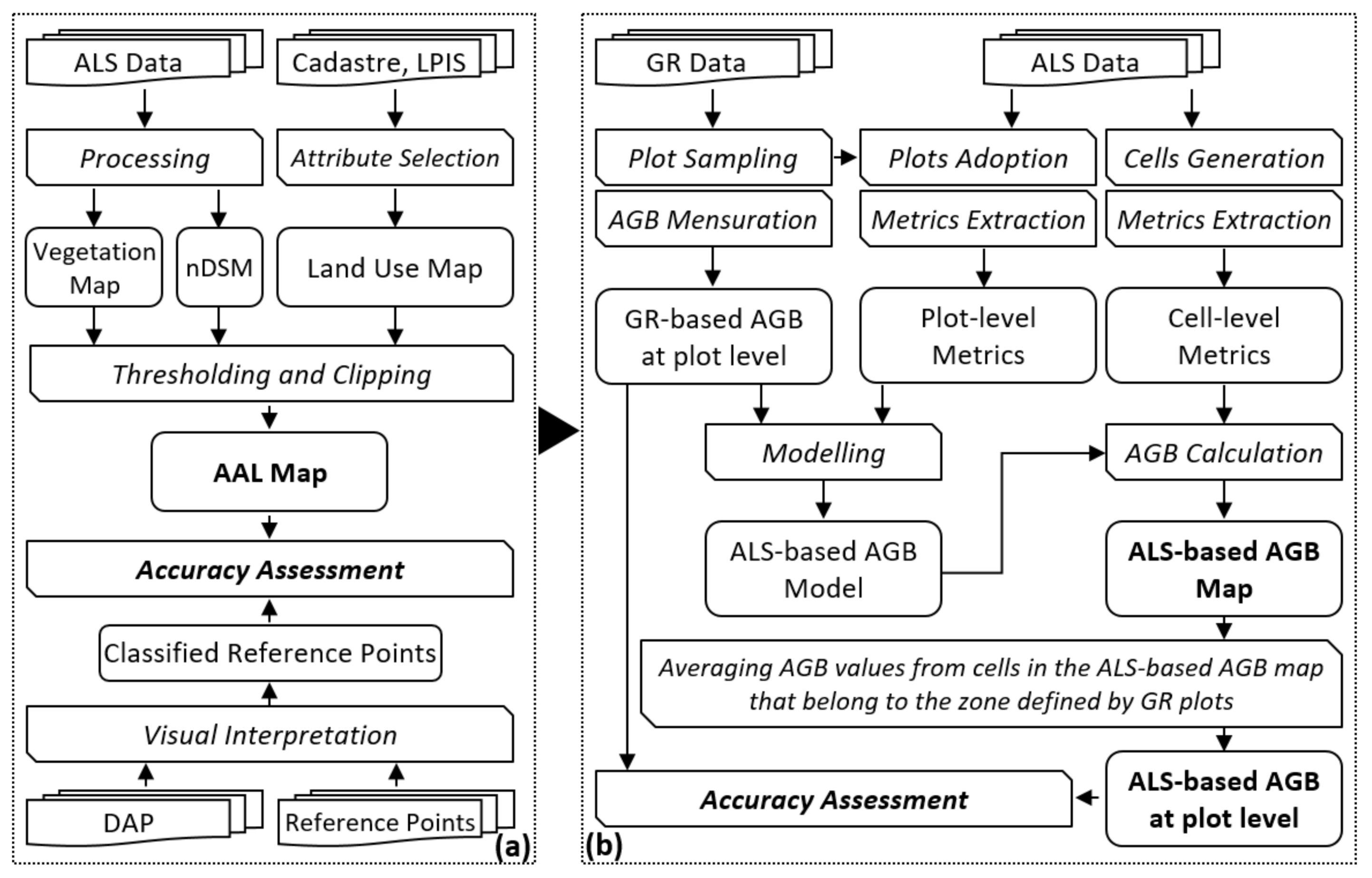
The workflow for mapping AGB on AAL based on a combination of field and ALS data is shown in Figure 2 and described in detail in the following sections.

2.4.1. Spatial Identification of Abandoned Agricultural Land

A vegetation class [47] was generated as a result of the classification and filtration of the ALS data. The process was conducted in the SCOP++ software environment (Trimble) using a robust filtering method [48]. The vegetation class was then used to create a vegetation map in raster format with a 0.5 m resolution representing the current state of total vegetation in the study area.
As the estimation of AGB was focused exclusively on AAL, we reduced the vegetation map in three consecutive steps (Figure 2a). For this purpose, we adopted the definition from [49,50], according to which agricultural land is generally represented by arable land, permanent crops, permanent meadows, and permanent pastures, while this agricultural land is considered to be abandoned when it has no longer has any farming functions. Firstly, we excluded forests, settlements, wetlands, and others (e.g., communications) using cadastral data. Secondly, we excluded farmland with active management using LPIS data. Finally, we removed pixels smaller than 1.5 m using nDSM. The height threshold was set to reflect the range of commonly accepted definitions of AAL classes [51] with the goal of ensuring that herbaceous formations were excluded from the final AAL map. In this way, we generated an AAL map of 0.5 m resolution that includes areas of AAL overgrown by medium-sized vegetation (shrub formations) and by tall vegetation (tree formations).

2.4.2. Mapping Aboveground Woody Biomass on Abandoned Agricultural Land

The ALS metrics from all 75 reference plots, as candidate variables for predictive AGB models, were computed from ALS data for specific areas of each reference plot using the author-developed submodule “Point Cloud Metrics” implemented in the reFLex software environment. In this study, we computed numerous height metrics, applying a 1.5 m height threshold (Table 3). The spatial location of plots was defined by a polygon shapefile.
The nonparametric model for AGB prediction was developed based on machine learning methods using the R package RandomForest [52]. The number of predictor variables performing the data partitioning at each node (mtry) was defined by the number of highly uncorrelated preliminary sets of ALS metrics, and the total number of trees to be grown in the model run (ntree) was set to 1000 because, in this setting, RF avoids unnecessary processing time [53]. Even though machine learning algorithms are usually not sensible for collinearity, normality, or linearity, in order to reduce a multicollinearity effect, we used two techniques for predictor selection. First, we used Pearson’s correlation analysis to identify highly correlated metrics that were related to each other as well as to ground-based AGB. Second, we used principal component analysis (PCA) to select a final set of predictor variables. In order to correctly apply PCA, we normalized the range of ALS metrics using the unit variance scaling technique. Here, we calculated the standard deviation for each variable and obtained the scaling weight as the inverse standard deviation. Subsequently, each variable was multiplied by the standard deviation; each scaled variable then had equal variance [54]. A correlation matrix derived from the normalized ALS metrics provided the basis for the eigenvalue and eigenvector calculations and for the subsequent determination of the principal component (PC) scores. By analyzing the eigenvectors and the PC score, we assessed the contribution of each ALS metric and used those with the highest loading on the PCs as the input variables for the final AGB model. Finally, the ALS-based AGB (AGB_ALS) was estimated using the developed predictive models within all reference plots.
The regular 20 × 20-m grid covering the area defined by the AAL map was created and the same metrics as in Table 3 were computed for all grid cells (85,648 cells). The size of the grid cells (400 m2) was set to reflect the size of the ground plots (314 m2) and to allow upscaling of the ALS-based estimations through satellite data in future work (e.g., Sentinel 1, Sentinel 2, and ALOS 2). The ALS-based AGB was predicted for all grid cells through the developed predictive RF model. In this way, the map of the ALS-based AGB with a pixel size of 20 m was generated, covering AAL across the whole study area.

2.4.3. Validation of the Models and Maps

The accuracy of the ALS-based spatial identification of AAL was assessed by an error matrix, including calculations of the producer’s, user’s, and overall accuracies, as well as the Cohen’s kappa [55]. We used five reference areas (1 × 1 km) located in the center, northwest, northeast, southwest, and southeast of the study area (Figure 1). A total of 11,194 reference points located within the reference areas in the regular grid (20 × 20 m) but not overlapping the excluded areas (e.g., forest) were applied to calculate the error matrix. For this purpose, we applied additional geospatial datasets (Section 2.3). Specifically, (1) reference points were displayed concurrently on RGB and each point was interpreted visually as representing the AAL class or another class and, independently, (2) reference points were displayed concurrently on the ALS-based AAL map and were automatically selected by location as representing the AAL class or another class.
The accuracy of the ALS-based mapping of AGB on AAL was assessed by comparing the ALS-predicted AGB (AGB_ALS) and the ground-observed AGB (AGB_GR). Here, we used all 75 reference plots. The value of AGB_GR for each reference plot was obtained by ground measurement (Section 2.1). The value of AGB_ALS for each reference plot was obtained using a zonal function in the ArcGIS environment (ESRI). Specifically, we calculated the average of all cells in the ALS-based AGB map (Section 2.4.2) that belong to the zone defined by the reference plot. We are convinced that the value of AGB extracted from the final map and not computed directly from the predictive model is sufficiently independent of the training data, and the proposed approach is an objective alternative to out-of-sample testing, such as cross-validation. Subsequently, bias (Equation (1)) and RMSE (Equation (2)) were used to assess the model’s performance. The relative %bias and %RMSE were calculated as the ratios of their absolute values and the arithmetic average of the reference data. Additionally, the regression function, coefficient of determination (R2), and F-test of statistical significance of the regression model (p-value) were calculated to assess the strength of the relationship between AGB_ALS and AGB_GR. Finally, we used (1) a t-test when a normal distribution of mean differences was confirmed or (2) a Wilcoxon test when a normal distribution of mean differences was not confirmed to assess the significance of differences (p-values < 0.05).
B i a s = 1 n i = 1 n ( y ^ i y i ) ,
R M S E = i = 1 n ( y ^ i y i ) 2 / n ,
where n is the number of reference (ground) plots, yi is the ground-observed AGB for plot i, and y ^ i is the ALS-predicted AGB that was extracted from the final AGB map for the area of plot i.

3. Results

3.1. Performance of the Spatial Identification of Abandoned Agricultural Land

In the error matrix of Table 4, the user’s, producer’s, and overall accuracies, as well as the Cohen’s kappa related to the ALS-based determination of AAL, are presented. The overall error, the error of omission, and the error of commission achieved values of 7.0%, 9.7%, and 7.8%, respectively.

3.2. Performance of Mapping the Aboveground Woody Biomass on Abandoned Agricultural Land

3.2.1. Predictor Variable Selection

A total of 17 of the 26 ALS metrics showed a very strong correlation (r > 0.9). In order to reduce any multicollinearity effect, we selected HP99 as one of the highly correlated metrics, because HP99 (1) approached the highest correlation to AGB (r = 0.94) and (2) provided the broadest combination of other remaining non-highly correlated metrics (r ≤ 0.9) (Table 5).
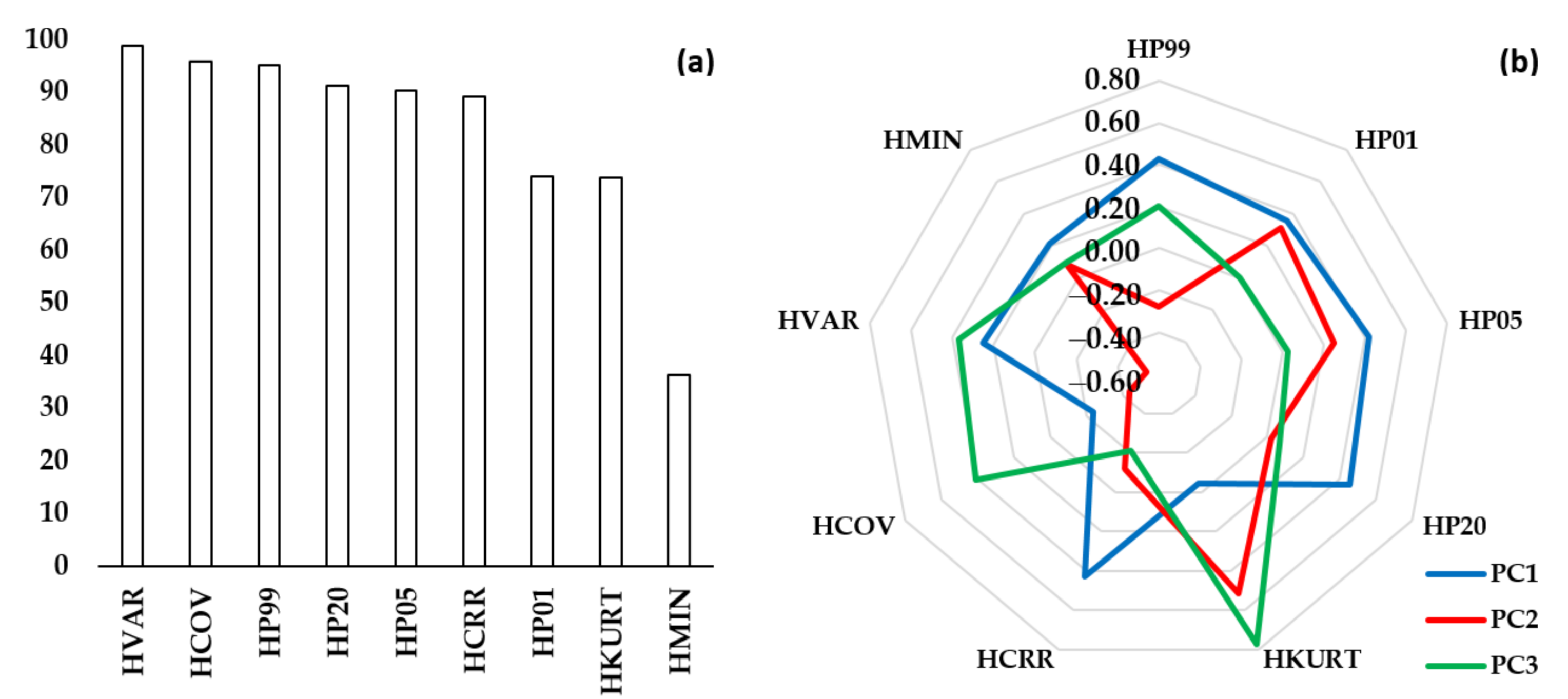
HP99, HP20, HP05, HP01, HMIN, HKURT, HCOV, HVAR, and HCRR were included in the PCA. The three PCs accounted for 94.6% of the total variance contained in the selected set of nine ALS metrics (PC1 = 63.0%, PC2 = 21.2%, and PC3 = 10.5%). The first PC was mainly influenced by height within different intervals and showed loadings by HP99, HP01, HP05, HP20, and HCRR. The second and third PCs were mainly influenced by height variability and showed loadings by HPKURT, HCOV, and HVAR. HMIN achieved minimal value of variable importance, loading as well as correlation to AGB (r = 0.2) and was discarded from the final model (Figure 3).

3.2.2. Accuracy of the AGB Map

The ALS-based approach evaluated the AGB at 227.0 ± 209.1 t ha−1 within the whole sample size, 38.8 ± 13.8 t ha−1 within the shrub–tree plots, and 349.8 ± 186.8 t ha−1 within the tree–shrub plots by using an RF model with eight predictors. The overall difference between the ALS-predicted and ground-observed AGB reached a relative RMSE at 26.1%, 33.1%, and 21.3% for the whole sample size, the shrub–tree plots, and the tree–shrub plots, respectively. Despite slightly underestimating the predictions, the ALS-predicted AGB in all samples did not differ significantly from the ground-observed AGB (p-values > 0.05) (Table 6). Moreover, the relationship between the ALS-predicted and ground-observed AGB was very high (R2 = 0.92) (Figure 4). A selected part of the AGB map is displayed in Figure 5.

4. Discussion

The motivation and hypothesis of this study focused on the presentation and assessment of a workflow for the spatial identification of AAL, and the mapping of AGB on identified AAL resulted mainly from the following points:
(1)
Uncontrolled cessation of agricultural production and the subsequent afforestation of agricultural land through forest succession is a serious challenge for the effective management of natural resources.
(2)
Mapping AGB on AAL is strictly required by relevant stakeholders (e.g., farmers, foresters, parcel owners, environmentalist, and policy-makers). This is primarily because these geospatial data make it possible to understand the state and trend of afforestation/deforestation in related regions and subsequently to implement a proper policy focused on the reduction of the negative effects of giving up agricultural production, support for sustainable forest management, or aimed at obtaining financial support.
(3)
RS technologies, especially ALS, represent an effective way to predict AGB on AAL and provide an opportunity to complement ground-based monitoring. Here, the ABA and RF models generally allowed us to obtain unbiased estimates of AGB and, in addition, the point density requirements of ALS data, hardware performance, and processing time are lower than with other methods.

4.1. Spatial Identification of Abandoned Agricultural Land

In this study, AAL was spatially identified based on an ALS-derived vegetation map, which was additionally corrected by cadastral and LPIS data. The overall accuracy of this process achieved a value of 93.00% (Cohen’s kappa = 0.82), and the final map of a 0.5 m resolution included farmland without agricultural activities and overgrown by shrub and tree formations. In this way, we have significantly improved the results of AAL identification, which would otherwise be related only to the commonly used data with limited spatial and temporal resolution (i.e., cadaster).
Comparable datasets and methods were used by [23,56,57,58,59]. These studies confirmed the applicability of ALS data from both leaf-on and leaf-off seasons, and the overall accuracy of the AAL map with a 1.0 m resolution was 90–95%. However, in all cases, an ancillary topographic database (e.g., cadaster) did not contain information about the state of agricultural activities, and in this case [23,59], the AAL was identified using object-based image analysis.
Most of the other studies tended to use optical images at various spatial resolutions to spatially identify AAL. This is because they are generally more accessible for large areas than ALS data. Here, an application of spectral or multiscale features extracted from aerial [60] or satellite images, such as GF-2 [61], Quick Bird [62], and Landsat [63], resulted in an overall accuracy of 77–91%. Several studies have also demonstrated the potential of radar data as an alternative to optical images for the identification of AAL. Synthetic aperture radar systems provided all-weather mapping capability [64], but the overall accuracy of AAL identification varied from 63% to 93% [18,65] and thus did not exceed the limits of optical images. Moreover, the limited spatial resolution of both optical and radar images may not be sufficient to identify the fragmented occurrence and dynamics of land abandonment.
In this context, our results showed that ALS data allowed us to map AAL with higher classification accuracy and spatial resolution than other RS platforms. Moreover, the process of AAL identification is largely automated and there is also a potential to improve the process of identification using some qualitative variable of ALS data (e.g., intensity) [66,67]. An application of multispectral ALS data could be very useful as well. Point clouds at three different laser wavelengths represent a new promising category of ALS data that could improve the results of land cover classification [68,69]. On the other hand, acquiring ALS data is associated with additional demands on budget and time, especially if a regular update at the regional/national level is requested. Here, the thorough and long-term preparation of flight missions should ensure the optimization of additional cost related to ALS application.

4.2. Mapping Aboveground Woody Biomass on Abandoned Agricultural Land

We proposed and assessed the workflow for the prediction of AGB on AAL comprising the techniques of ABA and machine learning, which are based on a combination of field and ALS data. The study findings showed that AGB located in specific areas of AAL can be predicted on the basis of the proposed workflow with a precision comparable to that obtained in other studies focusing on forest or shrub ecosystems.
The ALS-based AGB estimation reached a relative RMSE at 26.1% for all plots, 33.1% for plots with a predominance of shrub species, and 21.3% for plots with a predominance of tree species. Predictive models included field-observed AGB and a set of selected ALS data-calculated metrics. Specifically, we selected HP99, HP20, HP05, HP01, HKURT, HCOV, HVAR, and HCRR as the most important ALS metrics for AGB prediction. These metrics accounted for 94.6% of the total variation and the developed comprehensive RF model was unbiased for the whole sample size. Thus, there was no need to create two separate models, such as the shrub ecosystem-specific model and the tree ecosystem-specific model. In addition to the contribution of RF, this is primarily because the combination of selected ALS metrics precisely described the specific vertical structure of both shrub–tree plots and tree–shrub plots. First, while the shrub–tree plots contained more than 60% of the ALS points in the first quarter of the total height, most of the ALS points of the tree–shrub plots were located within the fourth quarter of the total height (Figure 6). Second, the height variability of the shrub–tree plots was nine times higher than the height variability of the tree–shrub plots, but AGB variability was relatively similar (Table 1). Here, a combination of HP99, HP20, HCOV, and HVAR was the most beneficial and sufficiently sensitive for the representation of different structural parameters of these vegetation formations (Figure 3). In addition, the suitability of most of these metrics has also been confirmed by other studies, such as [42] in Brazilian eucalyptus plantations (RMSE = 10–28%), [70] in Canadian boreal forests (RMSE = 20–29%), [71] in Chinese subtropical forests (RMSE = 22–23%), [72] in Spanish Mediterranean forests (RMSE = 3–39%), or [26] in the xeric shrub steppes of southwest Idaho (RMSE = 36–43%).
Although the application of ALS data in this study demonstrated sufficient applicability for mapping AGB on AAL, it is generally accepted that data fusion methods using multi-sensor RS data sources allow AGB predictions for large areas while maintaining accuracy and reducing the associated costs. For example, ALS-based AGB estimations could be expanded through data from Landsat-8 and Sentinel-1 [73,74], Landsat-7 [75], Sentinel-2 [76,77,78], as well as MODIS [79] sensors. The overall accuracy of AGB prediction varied from 25% [73] to 49% [79] in these studies. However, in all cases, the study area did not contain AAL. In this context, we include in the discussion our own and previously unpublished conclusions from a research project supported by the European Space Agency, entitled “Advanced Techniques for Biomass Mapping in Abandoned Agriculture Land using Novel Combination of Optical and Radar Remote Sensing Sensors”. The territory and time of the project realization is fully consistent with the territory and time of realization of this study. The methodology for AGB estimation and validation is similar, as well (i.e., Section 2.4.2 and Section 2.4.3). However, the AGB was predicted based on RF models consisting of ALS-based AGB prediction as the response variable and the predictor variables included a set of the selected metrics derived from multi-sensor satellite images (SAT), such as Sentinel 1 (leaf-off and leaf-on season), Sentinel 2 (leaf-off and leaf-on season), and ALOS 2 (leaf-off season). In this way, we developed three individual models for each sensor and one combined model for all sensors. In addition to the reasons mentioned in Section 2.4.2, RF was selected also for the SAT-based AGB prediction due to its ability to handle high-dimensional and non-normally distributed data. Here, a sample training dataset for the model development was created in a manner that allowed for the AGB class proportions of the training data to be representative of actual AGB class proportions in the landscape [80]. The overall accuracy of the SAT-based AGB estimation reached a relative RMSE at 60.1%, 62.1%, and 81.2% for the Sentinel-2, Sentinel-1, and ALOS-2. The predictive model consisting of selected metrics from all these sensors resulted in an overall accuracy of 62.1% in terms of relative RMSE. Specifically, all models provided a systematic overestimation in AGB prediction within the shrub–tree plots and a systematic underestimation in AGB prediction within the tree–shrub plots. Thus, the developed SAT-based models were not able to describe the specific structure of the shrub and tree ecosystems. We assume that the high variability in vegetation characteristics, especially the density and the height of the shrubs and trees, could be the main reason for the relatively high bias and RMSE values. The better results of the model based on Sentinel-2 data could be explained by the presence of broadleaved species in the study area, which led to a higher difference in winter and summer optical scenes compared to that of radar data. The lowest accuracy of the model based on ALOS 2 data probably resulted from only one scene used for model development, while Sentinel-1 scenes were available for the whole vegetation cycle (i.e., leaf-off as well as leaf-on seasons). There are several options to improve the results. For example, the possibility to include plots on managed agricultural land, as well as plots from young forest stands, into the training dataset could be tested to develop models with higher performance. Such an extended training dataset could help to train the models that more precisely describe the whole range of AGB distribution. The development of different ecosystem-specific (e.g., tree species group and vegetation type) models for the area of interest is also a promising solution. However, this should be an objective of a detailed study focused specifically on AGB prediction using multi-sensor satellite images.

5. Conclusions

This study selected an individual forest management unit located in central Slovakia that covered 12,472 ha as a study area to present the performance of the proposed workflow for mapping AGB on AAL based on ABA, RF models, and a combination of field and ALS data. The results in the context of existing studies indicate the following:
(1)
ALS data allowed for an automated and more accurate identification of AAL in terms of classification accuracy (>90%) and spatial resolution (<1.0 m) than did other RS platforms [53,54,55,56,57,58,59,60,61,62,63,64]. Potential improvements in process of AAL identification may be achieved using some qualitative variable of ALS data (e.g., intensity) or alternatively through multispectral ALS data [65,66,67,68]. The additional costs related to the application of ALS may be optimized by long-term survey planning.
(2)
Cadastral and LPIS data allowed us to apply the legal spatial status of parcels and to identify farmland without active agricultural activities. A combination of these data sources with the high-resolution ALS-derived map of vegetation resulted in more objective identification of AAL.
(3)
The authors’ algorithm implemented in the reFLex software was capable of providing relevant point cloud metrics (i.e., height) at the reference plot level (75 reference plots) as well as at forest management unit level (85,648 cells).
(4)
ALS data, despite a slight underestimation (bias from −2% to −6%), allowed more accurate prediction of AGB (RMSE < 33%) using ABA and the RF models than did other RS platforms [69,70,71,72,73,74,75]. Although the development of ecosystem-specific (e.g., tree species group and vegetation type) models is generally recommended, the single comprehensive RF model based on height metrics was sufficiently accurate for the whole area of interest (corresponding bias was not statistically significant). The additional costs related to obtaining the field data necessary for the development of the RF model may be optimized by the selection of a suitable sample design.
The description and performance assessment of the proposed workflow for mapping AGB on AAL presented herein can serve as useful information for relevant stakeholders related to the management of natural resources. We demonstrated that AAL can be identified and AGB on AAL can be predicted with relevant accuracy in large areas through ABA, nonparametric RF models, and a combination of field and ALS data. However, future research should include gradual testing of different RS data from active as well as passive sensors in different forest environments to assess their applicability for the practice of natural resource inventories.

Author Contributions

Conceptualization, I.S.; methodology and software, I.S.; data collection, I.B.; data process and analysis, I.S. and I.B.; writing—original draft preparation, I.S.; writing—review and editing, I.S.; project administration, I.S. and T.B.; funding acquisition, I.S. and T.B. All co-authors improved the article at various stages of the publication process. All authors have read and agreed to the published version of the manuscript.

Funding

This research was supported by the Slovak Research and Development Agency in the framework of the project “Development of advanced geospatial technologies for multiscale monitoring of forest ecosystems” (APVV-19-0257) as well as by the Government of Slovakia through an ESA Contract No. 4000123812/18/NL/SC under PECS (the views expressed herein can in no way be taken to reflect the official opinion of the ESA).

Acknowledgments

This study is the result of the project implementation: Centre of Excellence of Forest-based Industry (ITMS: 313011S735) supported by the Operational Programme Integrated Infrastructure funded by the ERDF.

Conflicts of Interest

The authors declare no conflict of interest.

References

  1. Alcantara, C.; Kuemmerle, T.; Prishchepov, A.V.; Radeloff, V.C. Mapping abandoned agriculture with multi-temporal MODIS satellite data. Remote Sens. Environ. 2012, 124, 334–347. [Google Scholar] [CrossRef]
  2. Kuemmerle, T.; Hostert, P.; Radeloff, V.C.; Van der Linden, S.; Perzanowski, K.; Kruhlov, I. Cross-border comparison of post-socialist farmland abandonment in the Carpathians. Ecosystems 2008, 11, 614–628. [Google Scholar] [CrossRef]
  3. Rey Benayas, J.; Martins, A.; Nicolau, J.M.; Schulz, J.J. Abandonment of agricultural land: An overview of drivers and consequences. CAB Rev. Perspect. Agric. Vet. Sci. Nutr. Nat. Resour. 2007, 2, 1–14. [Google Scholar] [CrossRef] [Green Version]
  4. Baumann, M.; Kuemmerle, T.; Elbakidze, M.; Ozdogan, M.; Radelo, V.C.; Keuler, N.S.; Prishchepov, A.V.; Kruhlov, I.; Hostert, P. Patterns and drivers of post-socialist farmland abandonment in Western Ukraine. Land Use Policy 2011, 28, 552–562. [Google Scholar] [CrossRef]
  5. Kumar, R.; Das, A.J. Climate change and its impact on land Degradation: Imperative need to focus. Climatol. Weather Forecast. 2014, 2, 2–4. [Google Scholar] [CrossRef]
  6. Goudriaan, J.; Unsworth, M.H. Impact of carbon dioxide, trace gases, and climate change on global agriculture. In Implications of Increasing Carbon Dioxide and Climate Change for Agricultural Productivity and Water Resources; Kimball, B.A., Ed.; American Society of Agronomy, Crop Society of America, and Soil Science Society of America: Madison, WI, USA, 1990; pp. 111–130. [Google Scholar]
  7. Queiroz, C.; Beilin, R.; Folke, C.; Lindborg, R. Farmland abandonment: Threat or opportunity for biodiversity conservation? A global review. Front. Ecol. Environ. 2014, 12, 288–296. [Google Scholar] [CrossRef]
  8. Goga, T.; Feranec, J.; Bucha, T.; Rusnák, M.; Sačkov, I.; Barka, I.; Kopecká, M.; Papčo, J.; Oťaheľ, J.; Szatmári, D.; et al. A review of the application of remote sensing data for abandoned agricultural land identification with focus on Central and Eastern Europe. Remote Sens. 2019, 11, 2759. [Google Scholar] [CrossRef] [Green Version]
  9. Li, W.; Wang, S.; Zhou, Y.; Xu, Q.; Wang, F.; Han, Y. Remote sensing methods for surveying and extracting abandoned farmlands. In Proceedings of the 2012 5th International Congress on Image and Signal Processing, Chongqing, China, 16–18 October 2012; pp. 1086–1090. [Google Scholar]
  10. Véga, C.; Renaud, J.; Durrieu, S.; Bouvier, M. On the interest of penetration depth, canopy area and volume metrics to improve Lidar-based models of forest parameters. Remote Sens. Environ. 2016, 175, 32–42. [Google Scholar] [CrossRef]
  11. Surový, P.; Kuželka, K. Acquisition of Forest Attributes for Decision Support at the Forest Enterprise Level Using Remote-Sensing Techniques—A Review. Forests 2019, 10, 273. [Google Scholar] [CrossRef] [Green Version]
  12. Kardoš, M.; Medveďová, A.; Supek, Š.; Škodová, M. Objektovo orientovaná klasifikácia drevinového zloženia na digitálnych leteckých snímkach zosuvného územia. Zprávy Lesnického Výzkumu 2013, 58, 195–205. (In Slovak) [Google Scholar]
  13. Ballanti, L.; Blesius, L.; Hines, E.; Kruse, B. Tree species classification using hyperspectral imagery: A comparison of two classifiers. Remote Sens. 2016, 8, 445. [Google Scholar] [CrossRef] [Green Version]
  14. Schlund, M.; Davidson, M.W.J. Aboveground forest biomass estimation combining L- and P-Band SAR acquisitions. Remote Sens. 2018, 10, 1151. [Google Scholar] [CrossRef] [Green Version]
  15. Brigot, G.; Simard, M.; Colin-Koeniguer, E.; Boulch, A. Retrieval of forest vertical structure from PolInSAR data by machine learning using LIDAR-derived features. Remote Sens. 2019, 11, 381. [Google Scholar] [CrossRef] [Green Version]
  16. Stefanski, J.; Chaskovskyy, O.; Waske, B. Mapping and monitoring of land use changes in post-Soviet western Ukraine using remote sensing data. Appl. Geogr 2014, 55, 155–164. [Google Scholar] [CrossRef]
  17. Wang, S.X.; Li, W.J.; Zhou, Y.; Wang, F.T.; Xu, Q.L. Object-oriented classification technique for extracting abandoned farmlands by using remote sensing images. In Proceedings of the 3rd International Conference on Multimedia Technology, Guangzhou, China, 29 November–1 December 2013; pp. 1497–1504. [Google Scholar]
  18. Yuso, N.M.; Muharam, F.M.; Takeuchi, W.; Darmawan, S.; Abd Razak, M.H. Phenology and classification of abandoned agricultural land based on ALOS-1 and 2 PALSAR multi-temporal measurements. Int. J. Digit. Earth 2017, 10, 155–174. [Google Scholar]
  19. Guenthert, S.; Siegmund, A.; Thunig, H.; Michel, U. Object-based detection of LUCC with special regard to agricultural abandonment on Tenerife (Canary Islands). In Proceedings of the Earth Resources and Environmental Remote Sensing/GIS Applications II, Prague, Czech Republic, 26 October 2011; Volume 8181, pp. 1–7. [Google Scholar]
  20. Löw, F.; Fliemann, E.; Abdullaev, I.; Conrad, C.; Lamers, J.P.A. Mapping abandoned agricultural land in Kyzyl-Orda, Kazakhstan using satellite remote sensing. Appl. Geogr. 2015, 62, 377–390. [Google Scholar] [CrossRef]
  21. Alcantara, C.; Kuemmerle, T.; Baumann, M.; Bragina, E.V.; Griths, P.; Hostert, P.; Knorn, J.; Müller, D.; Prishchepov, A.V.; Schierhorn, F. Mapping the extent of abandoned farmland in Central and Eastern Europe using MODIS time series satellite data. Environ. Res. Lett. 2013, 8, 035035. [Google Scholar] [CrossRef]
  22. Bożek, P.; Janus, J.; Mitka, B. Analysis of changes in forest structure using point clouds from historical aerial photographs. Remote Sens. 2019, 11, 2259. [Google Scholar] [CrossRef] [Green Version]
  23. Kolecka, N.; Kozak, J.; Kaim, D.; Dobosz, M.; Ostafin, K.; Ostapowicz, K.; Wezik, P.; Price, B. Understanding farmland abandonment in the polish Carpathians. Appl. Geogr. 2017, 88, 62–72. [Google Scholar] [CrossRef]
  24. Dube, T.; Mutanga, O.; Shoko, C.; Adelabu, S.A. Remote sensing of aboveground forest biomass: A review. Trop. Ecol. 2016, 57, 125–132. [Google Scholar]
  25. Barbosa, J.M.; Broadbent, E.N.; Bitencourt, M.D. Remote sensing of aboveground biomass in tropical secondary forests: A review. Int. J. For. Res. 2014, 715796, 1–14. [Google Scholar] [CrossRef]
  26. Li, A.; Dhakal, S.; Glenn, N.F.; Spaete, L.P.; Shinneman, D.J.; Pilliod, D.S.; Arkle, R.S.; McIlroy, S.K. Lidar aboveground vegetation biomass estimates in shrublands: Prediction, uncertainties and application to coarser scales. Remote Sens. 2017, 9, 903. [Google Scholar] [CrossRef] [Green Version]
  27. Askar, A.; Nuthammachot, N.; Phairuang, W.; Wicaksono, P.; Sayektiningsih, T. Estimating aboveground biomass on private forest using Sentinel-2 imagery. J. Sens. 2018, 2018, 1–11. [Google Scholar] [CrossRef]
  28. Liu, N.; Harper, R.J.; Handcock, R.N.; Evans, B.; Sochacki, S.J.; Dell, B.; Walden, L.L.; Liu, S. Seasonal timing for estimating carbon mitigation in revegetation of abandoned agricultural land with high spatial resolution remote sensing. Remote Sens. 2017, 9, 545. [Google Scholar] [CrossRef] [Green Version]
  29. Walden, L.L.; Harper, R.J.; Sochacki, S.J.; Montagu, K.D.; Wocheslander, R.; Clarke, M.; Ritson, P.; Emms, J.; Davoren, C.W.; Mowat, D.; et al. Mitigation of carbon following Atriplex nummularia revegetation in southern Australia. Ecol. Eng. 2017, 106, 253–262. [Google Scholar] [CrossRef] [Green Version]
  30. Helman, D.; Mussery, A.; Lensky, I.M.; Leu, S. Detecting changes in biomass productivity in a different land management regimes in drylands using satellite-derived vegetation index. Soil Use Manag. 2014, 30, 32–39. [Google Scholar] [CrossRef]
  31. Shen, W.; Li, M.; Huang, C.; Tao, X.; Li, S.; Wei, A. Mapping annual forest change due to afforestation in Guangdong province of China using active and passive remote sensing data. Remote Sens. 2019, 11, 490. [Google Scholar] [CrossRef] [Green Version]
  32. Maltamo, M.; Naesset, E.; Vauhkonen, J. Forestry Application of Airborne Laser Scanning: Concept and Case Studies; Springer: Dordrecht, The Netherlands, 2014; p. 460. [Google Scholar]
  33. Shinzato, E.T.; Shimabukuro, Y.E.; Coops, N.C.; Tompalski, P.; Gasparoto, E.A.G. Integrating area-based and individual tree detection approaches for estimating tree volume in plantation inventory using aerial image and airborne laser scanning data. iForest 2016, 10, 296–302. [Google Scholar] [CrossRef] [Green Version]
  34. Mauro, F.; Ritchie, M.; Wing, B.; Frank, B.; Monleon, V.; Temesgen, H.; Hudak, A. Estimation of changes of forest structural attributes at three different spatial aggregation levels in northern California using multitemporal LiDAR. Remote Sens. 2019, 11, 923. [Google Scholar] [CrossRef] [Green Version]
  35. Sibona, E.; Vitali, A.; Meloni, F.; Caffo, L.; Dotta, A.; Lingua, E.; Motta, R.; Garbarino, M. Direct measurement of tree height provides different results on the assessment of LiDAR accuracy. Forests 2017, 8, 7. [Google Scholar] [CrossRef]
  36. USDA Forest Services: FUSION/LDV LIDAR Analysis and Visualization Software. Available online: http://forsys.cfr.washington.edu/FUSION/fusion_overview.html (accessed on 18 August 2020).
  37. Rapidlasso GmbH: Fast Tools to Catch Reality. Available online: https://rapidlasso.com (accessed on 18 August 2020).
  38. Sačkov, I.; Hlásny, T.; Bucha, T.; Juriš, M. Integration of tree allometry rules to treetops detection and tree crowns delineation using airborne lidar data. iForest 2017, 10, 459–467. [Google Scholar] [CrossRef] [Green Version]
  39. Sačkov, I.; Kulla, L.; Bucha, T. A Comparison of Two Tree Detection Methods for Estimation of Forest Stand and Ecological Variables from Airborne LiDAR Data in Central European Forests. Remote Sens. 2019, 11, 1431. [Google Scholar] [CrossRef] [Green Version]
  40. Iizuka, K.; Hayakawa, Y.S.; Ogura, T.; Nakata, Y.; Kosugi, Y.; Yonehara, T. Integration of multi-sensor data to estimate plot-level stem volume using machine learning algorithms–case study of evergreen conifer planted forests in Japan. Remote Sens. 2020, 12, 1649. [Google Scholar] [CrossRef]
  41. Santopuoli, G.; Di Febbraro, M.; Maesano, M.; Balsi, M.; Marchetti, M.; Lasserre, B. Machine Learning Algorithms to predict tree-related microhabitats using airborne laser scanning. Remote Sens. 2020, 12, 2142. [Google Scholar] [CrossRef]
  42. Silva, V.S.; Silva, C.A.; Mohan, M.; Cardil, A.; Rex, F.E.; Loureiro, G.H.; Almeida, D.R.A.; Broadbent, E.N.; Gorgens, E.B.; Dalla Corte, A.P.; et al. Combined impact of sample size and modeling approaches for predicting stem volume in eucalyptus spp. forest plantations using field and LiDAR data. Remote Sens. 2020, 12, 1438. [Google Scholar] [CrossRef]
  43. Murgaš, V.; Sačkov, I.; Sedliak, M.; Tunák, D.; Chudý, F. Assessing horizontal accuracy of inventory plots in forests with different mix of tree species composition and development stage. J. For. Sci. 2018, 64, 478–485. [Google Scholar] [CrossRef] [Green Version]
  44. Petráš, R.; Pajtík, J. Sústava česko-slovenských objemových tabuliek drevín. Lesnícky Časopis 1991, 37, 49–56. (In Slovak) [Google Scholar]
  45. Konôpka, B.; Pajtík, J.; Šebeň, V. Biomass functions and expansion factors for young trees of European ash and Sycamore maple in the Inner Western Carpathians. Austrian J. For. Sci. 2015, 132, 1–26. [Google Scholar]
  46. EU. The Land Parcel Identification System: A Useful Tool to Determine the Eligibility of Agricultural Land–but Its Management could Be Further Improved. Special Report No. 25. 2016. Available online: https://op.europa.eu/en/publication-detail/-/publication/11049e0e-9a82-11e6-9bca-01aa75ed71a1 (accessed on 18 August 2020).
  47. ASPRS. LAS Specification 1.4. Available online: http://www.asprs.org/wp-content/uploads/2019/03/LAS14r14.pdf (accessed on 18 August 2020).
  48. INPHO. SCOP++. Available online: http://trl.trimble.com/docushare/dsweb/Get/Document-696440/022516-022B_Inpho_SCOP___TS_USL_0516_LR.pdf (accessed on 18 August 2020).
  49. FAO. FAOSTAT: Methods & Standards. Available online: http://www.fao.org/ag/agn/nutrition/Indicatorsfiles/Agriculture.pdf (accessed on 18 August 2020).
  50. Pointereau, P.; Coulon, F.; Girard, P.; Lambotte, M.; Stuczynski, T.; Sanchez Ortega, V.; Del Rio, A. Analysis of farmland abandonment and the extent and location of agricultural areas that are actually abandoned or are in risk to be abandoned. In JCR Scientific and Technical Reports; European Commission Joint Research Centre, Institute for Environment and Sustainability Press: Luxembourg, 2008. [Google Scholar]
  51. Perpiña, C.C.; Kavalov, B.; Diogo, V.; Jacobs-Crisioni, C.; Batista e Silva, F.; Lavalle, C. Agricultural Land Abandonment in the EU within 2015–2030; JRC113718; European Commission: Ispra, Italy, 2018; p. 7. [Google Scholar]
  52. Liaw, A.; Wiener, M. Classification and regression by random forest. R News 2002, 2, 18–22. [Google Scholar]
  53. Breiman, L. Random forests. Mach. Learn. 2001, 45, 5–32. [Google Scholar] [CrossRef] [Green Version]
  54. Eriksson, L.; Byrne, T.; Johansson, E.; Trygg, J.; Vikström, C. Multi- and Megavariate Data Analysis: Basic Principles and Applications; MKS Umetrics AB: Malmo, Sweden, 2013; p. 490. [Google Scholar]
  55. Kerr, G.H.G.; Fischer, C.; Reulke, R. Reliability assessment for remote sensing data: Beyond Cohen’s kappa. In Proceedings of the IEEE International Geoscience and Remote Sensing Symposium (IGARSS), Milan, Italy, 26–31 July 2015; pp. 141–152. [Google Scholar]
  56. Bożek, P.; Janus, J.; Taszakowski, J.; Głowacka, A. The use of Lidar data and cadastral databases in the identification of land abandonment. In Proceedings of the 17th International Multidisciplinary Scientific GeoConference SGEM, Vienna, Austria, 27–29 November 2017; pp. 705–712. [Google Scholar]
  57. Bożek, P.; Janus, J.; Lapa, P. The influence of the canopy height model methodology on determining abandoned agricultural areas. In Proceedings of the 17th International scientific conference Engineering for rural development, Jeglava, Latvia, 23–25 May 2018; pp. 795–800. [Google Scholar]
  58. Janus, J.; Bożek, P. Using ALS data to estimate afforestation and secondary forest succession on agricultural areas: An approach to improve the understanding of land abandonment causes. Appl. Geogr. 2018, 97, 128–141. [Google Scholar] [CrossRef]
  59. Hellesen, T.; Matikainen, L. An object-based approach for mapping shrub and tree cover on grassland habitats by use of LiDAR and CIR orthoimages. Remote Sens. 2013, 5, 558–583. [Google Scholar] [CrossRef] [Green Version]
  60. Morell-Monzó, S.; Estornell, J.; Sebastiá-Frasquet, M.T. Comparison of Sentinel-2 and high-resolution imagery for mapping land abandonment in fragmented areas. Remote Sens. 2020, 12, 2062. [Google Scholar] [CrossRef]
  61. Sun, B.; Gao, Z.; Zhao, L.; Wang, H.; Gao, W.; Zhang, Y. Extraction of information on trees outside forests based on very high spatial resolution remote sensing images. Forests 2019, 10, 835. [Google Scholar] [CrossRef] [Green Version]
  62. Liang, X.; Li, Y.; Zhou, Y. Study on the abandonment of sloping farmland in Fengjie County, Three Gorges Reservoir Area, a mountainous area in China. Land Use Policy 2020, 97, 104760. [Google Scholar] [CrossRef]
  63. Song, W. Mapping cropland abandonment in mountainous areas using an annual land-use trajectory approach. Sustainability 2019, 11, 5951. [Google Scholar] [CrossRef] [Green Version]
  64. Gašparović, M.; Dobrinić, D. Comparative Assessment of Machine Learning Methods for Urban Vegetation Mapping Using Multitemporal Sentinel-1 Imagery. Remote Sens. 2020, 12, 1952. [Google Scholar] [CrossRef]
  65. Goga, T.; Szatmári, D.; Feranec, J.; Papčo, J. Abandoned agricultural land identification using object-based approach and Sentinel data in the Danubian lowland, Slovakia. Int. Arch. Photogramm. Remote Sens. Spat. Inf. Sci. 2020, XLIII-B3-2020, 1539–1545. [Google Scholar] [CrossRef]
  66. Kolecka, N.; Kozak, J.; Kaim, D.; Dobosz, M.; Ginzler, C.; Psomas, A. Mapping secondary forest succession on abandoned agricultural land with LiDAR point clouds and terrestrial photography. Remote Sens. 2015, 7, 8300–8322. [Google Scholar] [CrossRef] [Green Version]
  67. Yan, W.Y.; Shaker, A.; El-Ashmawy, N. Urban land cover classification using airborne LiDAR data: A review. Remote Sens. Environ. 2015, 158, 295–310. [Google Scholar] [CrossRef]
  68. Ekhtari, N.; Glennie, C.; Fernandez-Diaz, J.C. Classification of airborne multispectral LiDAR point clouds for land cover mapping. IEEE J. Sel. Top. Appl. Earth Obs. Remote Sens. 2018, 11, 2068–2078. [Google Scholar] [CrossRef]
  69. Matikainen, L.; Karila, K.; Hyyppä, J.; Litkey, P.; Puttonen, E.; Ahokas, E. Object-based analysis of multispectral airborne laser scanner data for land cover classification and map updating. ISPRS J. Photogramm. Remote Sens. 2017, 128, 298–313. [Google Scholar] [CrossRef]
  70. Goodbody, T.R.; Tompalski, P.; Coops, N.C.; Hopkinson, C.; Treitz, P.; van Ewijk, K. Forest inventory and diversity attribute modelling using structural and intensity metrics from multi-spectral airborne laser scanning data. Remote Sens. 2020, 12, 2109. [Google Scholar] [CrossRef]
  71. Zhang, Z.; Cao, L.; She, G. Estimating forest structural parameters using canopy metrics derived from airborne LiDAR data in subtropical forests. Remote Sens. 2017, 9, 940. [Google Scholar] [CrossRef] [Green Version]
  72. Novo-Fernández, A.; Barrio-Anta, M.; Recondo, C.; Cámara-Obregón, A.; López-Sánchez, C.A. Integration of National Forest Inventory and Nationwide Airborne Laser Scanning Data to Improve Forest Yield Predictions in North-Western Spain. Remote Sens. 2019, 11, 1693. [Google Scholar] [CrossRef] [Green Version]
  73. Xie, B.; Cao, C.; Xu, M.; Bashir, B.; Singh, R.P.; Huang, Z.; Lin, X. Regional forest volume estimation by expanding LiDAR samples using multi-sensor satellite data. Remote Sens. 2020, 12, 360. [Google Scholar] [CrossRef] [Green Version]
  74. Sagang, L.B.T.; Ploton, P.; Sonké, B.; Poilvé, H.; Couteron, P.; Barbier, N. Airborne lidar sampling pivotal for accurate regional AGB predictions from multispectral images in forest-savanna landscapes. Remote Sens. 2020, 12, 1637. [Google Scholar] [CrossRef]
  75. Saarela, S.; Grafström, A.; Ståhl, G.; Kangas, A.; Holopainen, M.; Tuominen, S.; Nordkvist, K.; Hyyppä, J. Model-assisted estimation of growing stock volume using different combinations of LiDAR and Landsat data as auxiliary information. Remote Sens. Environ. 2015, 158, 431–440. [Google Scholar] [CrossRef]
  76. Puliti, S.; Saarela, S.; Gobakken, T.; Stahl, G.; Næsset, E. Combining UAV and Sentinel-2 auxiliary data for forest growing stock volume estimation through hierarchical model-based inference. Remote Sens. Environ. 2018, 204, 485–497. [Google Scholar] [CrossRef]
  77. Peters, D.L.; Niemann, K.O.; Skelly, R. Remote Sensing of Ecosystem Structure: Fusing Passive and Active Remotely Sensed Data to Characterize a Deltaic Wetland Landscape. Remote Sens. 2020, 12, 3819. [Google Scholar] [CrossRef]
  78. Plakman, V.; Janssen, T.; Brouwer, N.; Veraverbeke, S. Mapping Species at an Individual-Tree Scale in a Temperate Forest, Using Sentinel-2 Images, Airborne Laser Scanning Data, and Random Forest Classification. Remote Sens. 2020, 12, 3710. [Google Scholar] [CrossRef]
  79. Durante, P.; Martín-Alcón, S.; Gil-Tena, A.; Algeet, N.; Tomé, J.L.; Recuero, L.; Palacios-Orueta, A.; Oyonarte, C. Improving Aboveground Forest Biomass Maps: From High-Resolution to National Scale. Remote Sens. 2019, 11, 795. [Google Scholar] [CrossRef] [Green Version]
  80. Millard, K.; Richardson, M. On the importance of training data sample selection in random forest image classification: A Case Study in Peatland Ecosystem Mapping. Remote Sens. 2015, 7, 8489–8515. [Google Scholar] [CrossRef] [Green Version]
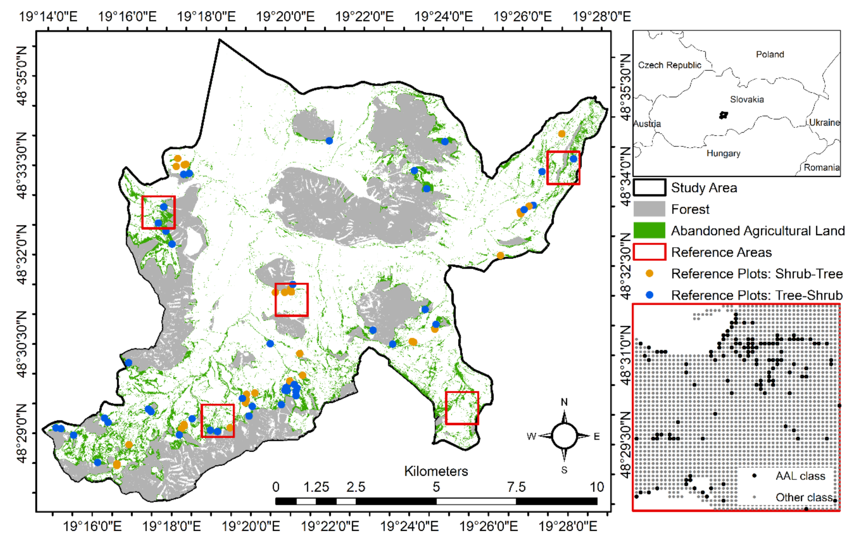
Figure 1. Study area, including 5 reference areas (reference points were visually interpreted and applied to assess the accuracy of the spatial identification of the abandoned agricultural land (AAL)) and 75 reference plots (shrub and tree vegetation was measured and reference data were used for the development of an airborne laser scanning (ALS)-based aboveground woody biomass (AGB) model and for assessing the performance of the AGB map). Reference plots were divided into two groups considering the relative dominance of shrub or tree species (ratio of the first group >75%).
Remotesensing 12 04189 g001
Figure 2. Flowchart for mapping aboveground woody biomass (AGB) on abandoned agricultural land (AAL): (a) Spatial identification of AAL; (b) mapping AGB on AAL. Note: ALS, airborne laser scanning; LPIS, land parcel identification system; nDSM, normalized digital surface model; DAP, digital aerial photography; GR, ground.
Remotesensing 12 04189 g002
Figure 3. Predictor variable selection: (a) Variable importance based on the random forest model; (b) eigenvector loadings based on principal component analysis. Note: PC, principal component.
Remotesensing 12 04189 g003
Figure 4. Relationship between the airborne laser scanning (ALS)-predicted and ground-observed aboveground woody biomass (AGB) in tons per hectare (t ha−1). The dashed line represents a 1:1 correspondence.
Remotesensing 12 04189 g004
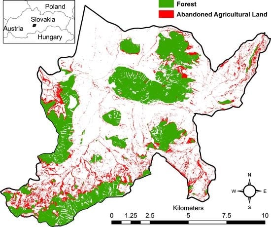
Figure 5. A map of the aboveground woody biomass (AGB) on abandoned agricultural land (north part of the study area).
Remotesensing 12 04189 g005
Figure 6. Density metrics of (a) shrub–tree plots and (b) tree–shrub plots. An airborne laser scanning data from each plot was divided into 10 height slices from low to high (RS01–10) and the proportion of returns in each slice is the corresponding density metric.
Remotesensing 12 04189 g006
Table 1. Summary statistics for the ground plots.
SamplesnA (ha)Canopy Height (m)AGB (t ha−1)
MeanStdMeanStd
All plots752.3615.3813.67231.51221.73
Shrub-tree plots *300.949.338.6641.0918.85
Tree-shrub plots *451.4236.003.56358.45203.09
Note: n, sample size; A (ha), area in hectares; Std, standard deviation. * Ratio of the first tree. species group >75%.
Table 2. An allometric model for quantifying aboveground woody biomass of shrubs on abandoned agricultural land.
Vegetation FormModel FormnA (m2)R2%RMSEp-Value
Shrubs speciesAGB = 1.2417 × h1.453612080.00.8123.94<0.001
Note: AGB, aboveground woody biomass, in kilograms per square meter; h, mean canopy height in meters; n, sample size; A, area in square meters; R2, coefficient of determination; %RMSE, root mean square error in percent; p-value of F-test, null hypothesis is rejected at α = 0.05.
Table 3. Airborne laser scanning canopy height metrics considered as candidate variables for the predictive aboveground woody biomass model.
VariableDescriptionVariableDescription
HMINHeight minimumHVARHeight variance
HMAXHeight maximumHSTDHeight standard deviation
HRANHeight range (H90-H10)HCOVHeight coefficient of variation
HCRRCanopy relief ratio (HMEAN-HMIN)/(HMAX-HMIN)HSKEWHeight skewness
HMEANHeight meanHKURTHeight kurtosis
HMODHeight modeHP01-99Height 1st–99th percentile
Table 4. Error matrix resulting from the spatial identification of the abandoned agricultural land (AAL).
Reference Data
ClassificationClassAALOtherTotalUser’s Accuracy (%)
AAL2672276294890.64
Other5087738824693.84
Total3180801411,194
Producer’s Accuracy (%)84.0396.56 93.00
Producer’s Accuracy: 90.29%; User’s Accuracy: 92.24%;
Overall Accuracy: 93.00%; Cohen’s Kappa: 0.82.
Table 5. Pearson correlations among the selected airborne laser scanning metrics.
HMINHCRRHVARHCOVHKURTHP01HP05HP20HP99
HMIN1
HCRR0.26 *1
HVAR0.170.50 ***1
HCOV−0.18−0.46 ***0.111
HKURT−0.10−0.28 *−0.26 *−0.151
HP010.37 **0.56 ***0.10−0.46 ***0.121
HP050.41 ***0.74 ***0.21−0.54 ***0.120.85 ***1
HP200.35 **0.89 ***0.49 ***−0.49 ***−0.010.69 ***0.88 ***1
HP990.33 **0.85 ***0.80 ***−0.20−0.180.52 ***0.70 ***0.89 ***1
Note: *** p < 0.001; ** p < 0.01; * p < 0.05. If there is no *, then p > 0.05.
Table 6. Differences between the airborne laser scanning (ALS)-predicted and ground-observed aboveground woody biomass.
Samplesn%bias%RMSENormality TestPaired Test
Wp-ValueZp-Value
All plots75−1.9326.050.720.000.560.57
Shrub–tree plots30−5.5733.050.920.040.340.73
Tree–shrub plots45−2.4321.320.780.000.020.98
Note: n, sample size; %RMSE, relative root mean square error; W, test statistic of the Shapiro–Wilk normality test; Z, test statistic of the Wilcoxon matched pairs test; p-value, null hypothesis is rejected at α = 0.05.
Publisher’s Note: MDPI stays neutral with regard to jurisdictional claims in published maps and institutional affiliations.