Abstract
Spatiotemporal fusion is considered a feasible and cost-effective way to solve the trade-off between the spatial and temporal resolution of satellite sensors. Recently proposed learning-based spatiotemporal fusion methods can address the prediction of both phenological and land-cover change. In this paper, we propose a novel deep learning-based spatiotemporal data fusion method that uses a two-stream convolutional neural network. The method combines both forward and backward prediction to generate a target fine image, where temporal change-based and a spatial information-based mapping are simultaneously formed, addressing the prediction of both phenological and land-cover changes with better generalization ability and robustness. Comparative experimental results for the test datasets with phenological and land-cover changes verified the effectiveness of our method. Compared to existing learning-based spatiotemporal fusion methods, our method is more effective in predicting phenological change and directly reconstructing the prediction with complete spatial details without the need for auxiliary modulation.
1. Introduction
Satellites with high temporal and spatial resolution are capable of capturing dynamics at a fine scale, obtaining dense remotely sensed time-series data that play an important role in studying the dynamics of earth systems, such as monitoring vegetation phenology [1], detecting land-cover changes [2], discriminating different land-cover types [3], and modeling carbon sequestration [4]. With the increase in the number of available satellite images, studies using dense time-series data have become extremely popular in this decade. However, a trade-off between the spatial and the temporal resolution of satellite sensors still exists due to limitations of the technology and budget constraints [5]. Spatiotemporal fusion methods, which combine different sensors, are considered a feasible and cost-effective way to solve this problem [6,7]. Specifically, spatiotemporal fusion methods combine high spatial and temporal resolution images to generate fused images under the condition that the two kinds of sensors have similar spectral properties.
In the past decade, various spatiotemporal fusion methods have been proposed. Among them, linear fusion methods are the most widely used type, and these are based on two hypotheses: (1) the relationship between the reflectance of fine (images with high spatial resolution but low temporal resolution) and coarse (images with low spatial resolution but high temporal resolution) images is linear; and (2) the temporal change between the reflectance of two coarse images is linear within a short period.
For the first hypothesis, the predicted images are obtained by applying this linear relationship between coarse and fine images to the coarse image at the prediction date. The Spatial and Temporal Adaptive Reflectance Fusion Model (STARFM) [5] is one of the earliest and most widely used linear spatiotemporal fusion methods, which is based on the premise that the reflectance of fine images is equal to the sum of the reflectance of a coarse image and a modulation term, representing the reflectance difference between the coarse and fine images. STARFM assumes that the modulation term is consistent; however, reflectance changes for pure pixels are supposed to be consistent between coarse and fine images, which is not applicable in heterogeneous areas [7,8]. To improve the fusion performance of STARFM in heterogeneous areas dominated by mixed pixels, an enhanced STARFM (ESTARFM) [8] method has been proposed, introducing a conversion coefficient to measure the temporal change rate of each class separately [9]. To apply the linear spatiotemporal fusion method to land-cover change, the Rigorously-Weighted Spatiotemporal Fusion Model with uncertainty analysis (RWSTFM) [10] uses linear regression to express the relationship between the reflectance of fine and coarse images and relax the assumption that the regression coefficient is consistent at different dates. In this model, the coefficient is updated using a correction factor.
For the second hypothesis, the predicted image is obtained by applying the linear relationship modeling the temporal change of two known coarse images to the known fine image. The Spatial and Temporal Non-Local Filter-based Fusion Model (STNLFFM) developed by Cheng et al. [11] is a typical example of this kind of method. First, given two coarse images acquired at different times, linear regression is utilized to express the temporal change, followed by obtaining the regression coefficients using the least squares method on neighboring pixels. Then, the coefficients are applied to the known fine image to obtain the prediction. To further decrease the effects of blocky artifacts caused by significant differences in the spatial resolution of the fine and coarse images, the method used similar pixels to formulate a non-local filter. Fit_FC, developed by Wang and Atkinson [12], employed a similar theoretical assumption as STNLFFM; the advantage of Fit_FC lies in the residual compensation for the further decrease of the uncertainty, which was generated during the linear regression of the two given coarse images. The Hybrid Color Mapping approach (HCM), developed by Chiman Kwan [13], also utilized the linear mapping between two known coarse images to express the temporal change information. However, different from the above two methods, the mapping extracted by HCM is based on the patches, instead of using the neighboring pixels. The Enhanced Linear Spatiotemporal Fusion Method (ELSTFM), proposed by Bo [14], replaced the linear regression coefficients with the residual term, which was obtained by spectral unmixing to obtain a more accurate prediction.
Due to its relatively simple implementation, linear spatiotemporal fusion methods have been utilized in various applications, such as land-cover classification [15,16], wetland monitoring [17], land surface temperature monitoring [18,19], leaf area index monitoring [20,21], and evapotranspiration monitoring [22,23]. However, this type of method has some major limitations: (1) linear theoretical assumptions are implausible in the case of land-cover change, resulting in poor fusion performance in land-cover change prediction; and (2) the effectiveness of linear spatiotemporal fusion methods depends on the selection of the weighting function, which is empirical with limited generalization [24].
Recently, proposed learning-based methods are no longer limited by the two linearity assumptions and can handle predictions of both phenological and land-cover change [25]. Therefore, these methods are expected to achieve better fusion performance, especially for land-cover change prediction [24]. The core of these methods is the formulation of the nonlinear mapping between the given pair of fine and coarse images based on their spatial structural similarity. The target fine images are generated by employing the learned nonlinear mapping to the corresponding coarse image [26]. Dictionary pair-based methods are representative learning-based methods, which introduced non-local similarities and non-analytic optimization in the sparse domain to predict the fine image. The Sparse-representation-based Spatiotemporal Reflectance Fusion model (SPSTFM) [26], developed by Huang, is an initial example of dictionary pair-based methods, which formulated the nonlinear mapping between the fine and coarse image by jointly training two dictionaries from fine and coarse image patches. Then, the one-pair learning method was further developed to apply the SPSTFM method to the case of one known pair of fine and coarse images [27]. Since SPSTFM’s assumption that the sparse coefficients across the fine and coarse image patches are the same is too strict, subsequent studies have been devoted to relaxing this assumption, such as the error-bound-regularized sparse coding (EBSPTM) [28], block Sparse Bayesian Learning for Semi-Coupled Dictionary Learning (bSBL-SCDL) [29], and compressed sensing for spatiotemporal fusion (CSSF) [30]. Although these dictionary pair-based methods can predict both the phenological and land-cover changes, the high computational complexity of sparse coding limits their applicability. To reduce this complexity, the extreme learning machine (ELM), a fast single hidden layer feed-forward neural network, was utilized to learn the nonlinear mapping between the fine and coarse images [31]. Motivated by the advantages of deep nonlinear mapping learning, some relevant spatiotemporal fusion methods have been proposed [32,33]. The Deep Convolutional Spatiotemporal Fusion Network (DCSTFN) [32] used a convolutional neural network (CNN) to extract the main frame and background information from the fine image and the high-frequency components from coarse images. Then, using the hypothesis equation from STARFM, two types of extracted features are merged to generate the final prediction. Although DCSTFN outperforms conventional spatiotemporal fusion methods in generalization ability and robustness, since the method is still based on the linearity assumption, its ability to handle predictions with land-cover change is limited.
Recently, Song et al. [33] devised a multi-step spatiotemporal fusion framework with Deep Convolutional Neural Networks (STFDCNN), in which an effective deep learning-based single image super-resolution method (SRCNN) was utilized to form the nonlinear mapping and apply super-resolution in sequence. Although the method can achieve reasonable fusion performance, both the nonlinearity mapping and super-resolution step based on the SRCNN fail to reconstruct the spatial details of the predictions, as they are dependent on an additional high-pass modulation. Additionally, the method focused on formulating the nonlinear mapping, whereas no physical temporal change information was taken into account.
In light of the above limitations, we propose a novel deep learning-based spatiotemporal data fusion method (DL-SDFM) using a two-stream convolutional neural network. The main advantages of DL-SDFM include the following:
- DL-SDFM addresses the prediction of both phenological and land-cover changes with high generalization ability and robustness.
- DL-SDFM enriches the learning-based spatiotemporal fusion method with temporal change information, resulting in a more robust ability of predicting the phenological change compared to the existing learning-based spatiotemporal fusion methods.
- DL-SDFM can directly reconstruct the prediction with complete spatial details without the need for auxiliary modulation.
2. Methods
We refer to images with low spatial resolution but high temporal resolution as “coarse” images, while images with high spatial resolution but low temporal resolution are called the “fine” images. In this paper, we consider both forward and backward prediction to generate a target fine image with higher robustness, given two coarse and fine image pairs ( and , and ) and a corresponding coarse image (Figure 1).
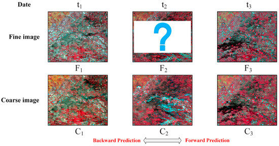
Figure 1.
Images for spatiotemporal fusion. Coarse images were obtained at , , and , while fine images are available for and , and the fine image at is the target image.
The flowchart of DL-SDFM is shown in Figure 2. In forward prediction, a temporal change-based and a spatial information-based mapping (, ) are built simultaneously using a two-stream convolutional neural network, taking two coarse and fine image pairs as inputs. Then, using the two learned mappings, two independent predictions () of the phenological and land-cover changes respectively are obtained. The final forward prediction is generated by combining the above two independent predictions using a weighted method. Then, backward prediction is implemented in the same fashion, i.e., a temporal change-based and a spatial information-based mapping (, ) are built simultaneously, followed by obtaining the two independent predictions (, ) for backward prediction. The final backward prediction is generated by combining the two independent predictions, while the target fine image is obtained through the combination of the forward and the backward prediction. A detailed description of each step of DL-SDFM is given below.
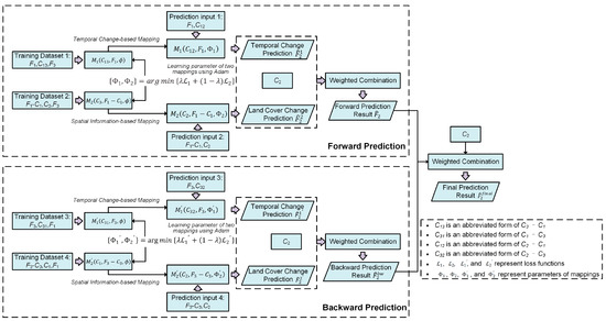
Figure 2.
Flowchart of deep learning-based spatiotemporal data fusion method (DL-SDFM).
2.1. Temporal Change-Based Mapping
Existing learning-based spatiotemporal fusion methods do not introduce the physical temporal change information. To augment the learning-based spatiotemporal fusion method with temporal change information and develop a more powerful ability to predict phenological change, we formulate the temporal change-based mapping.
Suppose that the changes of reflectance from date to are linear. If the period is short, the coarse image at can be described as
where denotes the coarse image, is a given pixel location at band at two different dates, while and are the coefficients of the linear regression model that describe the temporal change of the reflectance of the coarse image between and . Since the coarse image has similar spectral bands to the fine image, the linear relationship between the two known coarse images ( and ) can be applied to the fine image at to obtain the target fine image :
The coefficients and can be estimated using the least squares method in a moving window. However, this will increase the computational cost. Therefore, we assume that is equal to 1 to reduce the computational cost, so the target fine image at can be calculated as
In this case, Equation (3) is equal to the basis of STARFM. If we further introduce a conversion coefficient into (3) to apply the method to the spatial heterogeneity regions, the target fine image at can be calculated as
Equation (4) is equal to the basis of ESTARFM. From the above analysis, the above methods can be summarized as the following mapping:
where is the mapping function and represents the temporal change information. The mapping function is a predefined weighting function in a moving window. Although the effectiveness of in the prediction of phenological change has been verified, since it is difficult to accurately model the complex and nonlinear relationships between the central and neighboring information, the generalization of these methods with such an artificial and predefined weighting function can be improved.
For a more adequate characterization of the complex and nonlinear mapping function to improve the fusion performance in phenological change prediction, in this paper, we leverage the CNN’s capability in nonlinear mapping representation to formulate a nonlinear mapping for phenological change prediction and learning of the self-adaption weights.
Specifically, for forward prediction, we consider as the label, and the temporal change information and the known fine image as the inputs. The mapping is learned via the proposed two-stream convolutional neural network (Section 2.3):
where is the parameter of mapping , is the defined loss function, and is an abbreviated form of , which represents the temporal change information.
2.2. Spatial Information-Based Mapping
The mapping can be regarded as the linear-based spatiotemporal fusion with prior images, focusing on the view of temporal change. Although the self-adaption weight learned by the CNN has more powerful generalization ability than the traditional linear-based spatiotemporal fusion methods, since the basis of is the same as that of STARFM, it also lacks the ability to address the predictions with land-cover change. Therefore, for the latter, we further formulate the mapping , which can directly reconstruct the spatial detail.
Learning-based spatiotemporal fusion methods are considered to have a stronger ability to predict land-cover change. These methods first formulate the complex mapping between the coarse and fine images based on spatial structural similarity and then use the learned mapping to predict the target fine image. Given two fine and coarse image pairs and , and , the nonlinear mapping between the fine and coarse images can be defined as
Although the above mapping endows the spatiotemporal fusion method with the capacity of predicting land-cover change, the magnification factor in spatiotemporal fusion is more significant than in single-image super-resolution (usually ranging from 2 to 4 in single-image super-resolution). In this case, texture details are severely blurred and distorted in coarse images. Thus, it may not be useful to reconstruct the spatial details directly using the above mapping.
To improve the above mapping’s ability to directly reconstruct the spatial details, we introduce the spatial difference information between fine and coarse images, which is expressed by , into the mapping (Equation (7)) to formulate the mapping . Note that the spatial difference information, which is also expressed as high-frequency information, has been shown to be useful in reconstructing the spatial detail [27]. For the mapping in forward prediction, we regard as the label, and the spatial differences information and the known coarse image as the inputs. Similarly, the nonlinear mapping is also learned by the proposed two-stream convolutional neural network.
where is the parameter of mapping , and is the defined loss function.
2.3. Network Architecture
In this paper, we propose a relatively lightweight two-stream CNN with a dilated convolution-based inception module to simultaneously learn the mappings and . The network consists of three stages: (1) multi-scale feature extraction; (2) multi-source feature fusion; and (3) image reconstruction. The overall architecture and the configuration of the network are provided in Figure 4 and Table 1, respectively. A detailed description of each stage is given below.

Table 1.
Detailed network configuration.
(1) Multi-scale feature extraction
Remote sensing images with high spatial heterogeneity contain abundant texture details, where the size of ground objects varies greatly. Thus, it is effective to use the rich multi-scale spatial information to improve the robustness of the feature extraction in these areas. To capture multi-scale spatial information, the GoogLeNet inception module proposed by Szegedy et al. [34] concatenates the outputs of different-sized filters, e.g., 3 × 3, 5 × 5, 7 × 7, assuming that each filter can capture information at the corresponding scale. Recently, the inception module has been utilized for image reconstruction and fusion tasks and has achieved state-of-the-art performance [35,36,37]. However, the increase of the size of the filters will inevitably result in an increase of parameters, which may not be appropriate in the case of the insufficient prior images (in our case, only two fine and coarse image pairs are available for training for the spatiotemporal fusion task).
Inspired by the GoogLeNet inception module, Shi [38] proposed the dilated convolution-based inception module to capture multi-scale information. In contrast to conventional convolutions, dilated convolutions enlarge the receptive field and maintain the size of the convolution kernel filter to avoid the increase of parameters. Dilated convolution employs the same filter at different ranges with different dilation factors, which allows it to capture multi-scale spatial information without increasing the parameters. As illustrated in Figure 3, the three dilated convolutions in the dilated convolution-based inception module can capture the multi-scale spatial information (see the pixels in blue), whilst operating on the same scale.
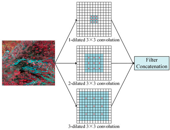
Figure 3.
Architecture of the dilated convolution-based inception module.
In this paper, we utilize this module to capture multi-scale spatial information. As shown in Figure 4, the three dilated convolutions with kernel size 3 × 3 and dilation factors 1, 2, and 3 are simultaneously applied on the input image and produce feature maps of 64 channels, followed by concatenation into a single 192-channel feature map. Then, a conventional convolution with kernel size 3 × 3 is performed on the concatenated output and 64 feature maps are generated. A rectified linear unit (ReLU) is used after each convolution layer to introduce nonlinearity and to speed up the convergence of the network.
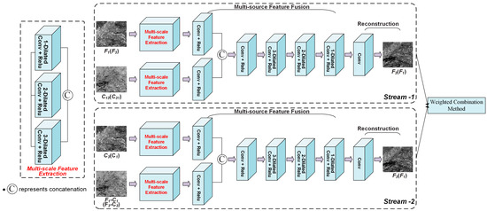
Figure 4.
Architecture of the two-stream convolutional neural network.
(2) Multi-source feature fusion
After capturing the multi-scale spatial information of fine and coarse image pair using the dilated convolution-based inception module, the extracted multi-scale information is concatenated into a single 384-channel feature map, followed by conventional convolution with kernel size 3 × 3, generating 64 feature maps.
However, a “gridding” issue [39] usually exists in the dilated convolution framework, which means that layers with an equal dilation factor may result in the loss of a large portion of information. A hybrid dilated convolution module [39] is a simple solution to address this issue, which uses a combination of dilated convolutions with different dilation factors to cover a square region without missing information. For more detailed descriptions of the “gridding” issue and the hybrid dilated convolution module, we refer the reader to [39].
To further enlarge the receptive field for extracting more contextual information while avoiding the “gridding” issue, a hybrid dilated convolution module is introduced in the multi-source feature fusion, where three dilated convolutions are applied with a kernel size of 3 × 3 and dilation factors of 1, 2, and 3, generating 64 feature maps. A ReLU is used after each convolution layer. This process can be described as:
where represents the convolution operation, while , , and represent the feature maps, filters, and biases of the n-th dilated convolutions in the multi-source feature fusion stage.
(3) Image Reconstruction
In the image reconstruction stage, conventional convolution with a kernel size of 3 × 3 and a filter is utilized to generate the final output.
Given two pairs of fine and coarse image ( and and ), we formulate the objective function of the proposed network as follows:
Here, and denote the network parameters of mappings and , is the weighting parameter, and and are the losses of two networks, which are denoted as:
where is the mean square error (MSE)-based loss function.
2.4. Prediction Stage
Based on the two learned mappings ( and ), for the forward prediction, we obtain two independent predictions (), focusing on phenological and land-cover change, respectively. One pair of known fine and coarse images ( and ) and a coarse image () at prediction date are taken as the inputs:
Since the two mappings are based on temporal change and spatial information respectively, the two independent predictions and may have different applicability under different scenarios. Here, we employ a weighted combination method to synthesize the two independent predictions, giving DL-SDFM the ability to predict both phenological and land cover change.
Under ideal conditions, the weight of the weighted combination method can be determined using the bias between the two predictions and the actual fine image; however, the actual fine image is unknown. Thus, we utilize the corresponding coarse image at the prediction date instead of the actual fine image to determine the weight. Meanwhile, to reduce the prediction errors caused by the inconsistency of spatial resolution between fine and coarse images, the weight measurement is implemented in a 3 × 3 moving window as follows:
where and are the reflectance of the j-th pixel of the two independent predictions in a 3 × 3 moving window, centered on pixel , while is the corresponding reflectance of the j-th pixel of the coarse image at the prediction date. Then, the final prediction can be obtained using:
2.5. Combination with Backward Prediction
The method described above only focuses on forward prediction. To improve robustness through the combination of both forward and backward predictions, we further consider the backward prediction. Accordingly, is regarded as the label in the training stage of the backward prediction. The two mappings in backward prediction are also simultaneously learned by the two-stream convolutional neural network:
where and denote the network parameters of the two mappings and for backward prediction, and is defined as . Similar to the prediction stage in the forward prediction, the two independent backward predictions , and the final backward prediction are obtained by:
where and denote the weights of the two independent backward predictions.
To combine the forward and backward predictions and obtain the final prediction, we utilize the same weighted combination method based on a 3 × 3 moving window as described in Section 2.4.
where and denote the weight of the forward and backward predictions, which are determined by the bias between the two predictions and the coarse image at the prediction date.
3. Experiment
3.1. Study Area and Data Sets
The performance of DL-SDFM was tested on two study sites to verify the effectiveness of the land-cover change and temporal change prediction, respectively.
The first study site was the Lower Gwydir Catchment (LGC), which is located in northern New South Wales, with an overall area of 5440 km2 (3200 × 2720 pixels in Landsat images with six bands). Since a large flood occurred in mid-December 2004, leading to the significant changes in land cover, it is reasonable to use this study site for testing the effectiveness of DL-SDFM on land-cover change prediction.
The dataset in this study site is the same as the one used by Emelyanova et al. [9]. In this experiment, we used two MODIS MOD09GA Collection 5 and Landsat 7 ETM+ image pairs acquired on 26 November 2004, and 28 December 2004, respectively, and a MODIS image acquired on 12 December 2004, to predict the fine Landsat image acquired on 12 December 2004, while the actual Landsat image acquired on that date was used to evaluate the fusion performance (Figure 5). MODIS images were upsampled from 500 m to the same spatial resolution as the Landsat images (25 m) using a nearest neighbor algorithm.
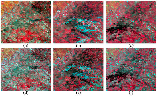
Figure 5.
Test images at the Lower Gwydir Catchment (LGC) site: MODIS images acquired on (a) 26 November 2004, (b) 12 December 2004, and (c) 28 December 2004; (d) Landsat images acquired on 26 November 2004, (e) 12 December 2004, and (f) 28 December 2004.
The second study site was located in a heterogeneous rain-fed agricultural area in central Iowa (CI), USA that has an overall area of 18,225 km2 (4500 × 4500 pixels in Landsat images with 6 bands) with an obvious phenological change area. We chose this study site to test the performance of DL-SDFM in spatially heterogeneous areas with visible phenological change. Two MODIS MOD09GA Collection 6 and Landsat 7 ETM+ image pairs acquired on 14 May 2002, and 2 August 2002, along with the MODIS image acquired on 2 July 2002, were utilized to predict the Landsat image acquired on 2 July 2002. As before, the actual Landsat obtained on 2 July 2002 was utilized to evaluate the fusion performance (Figure 6). MODIS images were upsampled from 480 m to the same spatial resolution as the Landsat images (30 m) using a nearest neighbor algorithm.
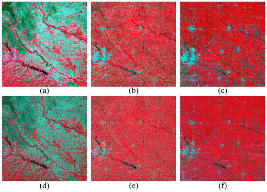
Figure 6.
Test images at the central Iowa (CI) site: MODIS images acquired on (a) 14 May 2002, (b) 2 July 2002, and (c) 2 August 2002. (d) Landsat images acquired on 14 May 2002, (e) 2 July 2002, and (f) 2 August 2002.
3.2. Parameter Setting
In the training stage, all the input images of the two mappings were cropped to 50 with a stride of 50. The parameter was fine-tuned by comparing all these parameters, namely {30, 40, 50, 60} to obtain the lowest root mean square error (RMSE) on the test datasets. To avoid over-fitting, multi-angle image rotation (angles of 0°, 90°, 180°, and 270°) was utilized to increase the training sample size. For optimization, the proposed network was trained using the Adam algorithm [40] as the gradient descent optimization method with momentum ,, and , which is the same as that used by Yuan et al. [41]. The batch size was set to 64 to fit into the GPU memory. The learning rate α was initialized to 0.0001 for the whole network, which was determined by comparing all these parameters, namely {0.00001, 0.0001, 0.001, 0.01} to obtain the lowest RMSE on the test datasets. The training process lasted 60 epochs to ensure convergence. After every 10 epochs, the learning rate was multiplied by a descent factor of 0.5. We employed the Keras deep learning library with TensorFlow to train the network on a PC with 32 GB RAM, an i7-7700k CPU, and an NVIDIA GTX 1070 GPU.
In the prediction stage, we cropped input images into patches of size 600 × 600 pixels to fit into the GPU memory. Meanwhile, to avoid boundary artifacts, we ensured that adjacent patches overlapped.
3.3. Comparison and Evaluation Strategy
(1) Comparison with other fusion methods
To verify the superiority of DL-SDFM, three state-of-the-art spatiotemporal fusion methods, including STARFM, Flexible Spatiotemporal Data Fusion (FSDAF), and STFDCNN, were utilized as benchmark methods. Fusion results were quantitatively and visually evaluated by comparing the prediction with the actual fine image acquired at the prediction date. For the quantitative evaluation, six indices were used: RMSE, correlation coefficient (CC), universal image quality index (UIQI) [42], the structural similarity (SSIM) [43], erreur relative global adimensionnelle de synthèse (ERGAS) [44], and the spectral angle mapper (SAM) [45].
RMSE was used to provide a global metric of the radiometric differences between the predicted and the actual fine image. CC was used to show the linear relationship between the prediction and the actual fine image. SSIM was used to show the similarity of the overall structure between the predicted and the actual fine image. UIQI depicts the closeness between the two images utilizing the differences in the statistical distributions. SAM reflects the spectral fidelity of the prediction, while ERGAS measures the overall fusion result. The ideal values of RMSE, CC, SSIM, and UIQI are 0, 1, 1, and 1, respectively, while smaller values for ERGAS and SAM indicate better fusion performance. Additionally, the average Average Absolute Difference (AAD) maps of the six bands between the actual fine image and fusion results were calculated, which represent the spatial distribution and magnitude of the predictions’ uncertainty. The closer the AAD was to zero, the less the uncertainty of predictions.
(2) Effectiveness of the fusion of temporal change information with spatial information
In DL-SDFM, the two independent predictions focusing on the phenological and land-cover change were combined with a weighted combination in a moving window. To verify the effectiveness of this combination, we compared the quantitative results of the two independent predictions and the combination results in DL-SDFM. The quantitative evaluation indices include RMSE, CC, SSIM, UIQI, SAM, ERGAS, and the average AAD maps.
(3) Effectiveness of the reconstruction of the spatial detail
To verify the effectiveness of DL-SDFM in spatial detail reconstruction, taking the prediction result of band 4 as an example, we further compared the spatial detail of the predictions of STFDCNN and DL-SDFM in both two study sites. For STFDCNN, in addition to the final prediction, its spatial detail of the nonlinear mapping result and the super-resolution result were also compared. The peak signal-to-noise ratio (PSNR), a common quantitative evaluation index in super-resolution, was used to give an evaluation of the image distortion, where a higher value indicates a better prediction [46].
3.4. Experimental Results
3.4.1. Prediction with Land-Cover Change
(1) Comparison with other fusion methods
The results of different fusion methods for the LGC site are shown in Figure 7, with the sub-areas inundated by floods zoomed to show more details. It can be seen that the predictions of STARFM provide the worst results with blurry texture details, while incomplete boundaries with some noise were generated for the inundated areas. The average AAD maps of STARFM (Figure 8b) further demonstrate that STARFM fails to handle the image with obvious land-cover change. As shown in Figure 7d and Figure 8c, FSDAF produces more precise texture details than STARFM, capturing more complete spatial variation with less noise in the edge of inundated areas. However, some artifacts still exist in some heterogeneous areas. STFDCNN yields complete spatial details, except for the inundated areas, where obvious blocky artifacts can be seen near the edges.
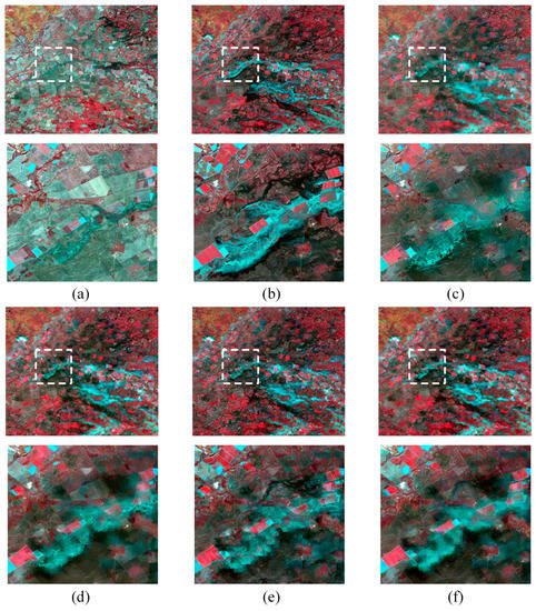
Figure 7.
Comparison of predicted and actual images at the LGC site. (a) Prior image acquired on 26 November 2004. (b) Actual image acquired on 12 December 2004. (c) Prediction result of Spatial and Temporal Adaptive Reflectance Fusion Model (STARFM). (d) Prediction result of Flexible Spatiotemporal Data Fusion (FSDAF). (e) Prediction result of spatiotemporal fusion framework with Deep Convolutional Neural Networks (STFDCNN). (f) Prediction result of deep learning-based spatiotemporal data fusion method (DL-SDFM).
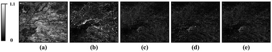
Figure 8.
Average Absolute Difference (AAD) maps of the six bands between the actual image and prediction results in the LGC site. (a) Actual image and prior Landsat image acquired on 26 November 2004. (b) Actual image and STARFM prediction. (c) Actual image and FSDAF prediction. (d) Actual image and STFDCNN prediction. (e) Actual image and DL-SDFM prediction.
In contrast, as shown in Figure 7f and Figure 8e, the DL-SDFM generates a prediction with relatively good spatial details, less uncertainty, and clear texture. Moreover, compared to the prediction of STFDCNN, a more complete boundary of the inundated area was generated, suggesting the superiority of the DL-SDFM in predictions with obvious land-cover change.
Quantitative results of the different fusion methods are shown in Table 2. It can be seen that STARFM provides the worst performance for all metrics, which is mainly due to the failure in predicting the inundated area (Figure 7c). FSDAF generates good results with considerably better values for all metrics. Compared to the FSDAF, STFDCNN is significantly better in the fusion accuracy for band 5 and band 7. Considering that band 5 changes the most when a flood occurs, this result indicates the superiority of the STFDCNN for predictions with land-cover change. Nevertheless, the DL-SDFM provides the best performance for all six bands, with the maximum similarity to the actual image and the best spectral fidelity, suggesting that the DL-SDFM is more powerful in making predictions involving land-cover change.
Table 2.
Quantitative results of different fusion methods applied to the LGC site. Bold indicates the best result. CC: correlation coefficient, ERGAS: erreur relative global adimensionnelle de synthèse, RMSE: root mean square error, SAM: spectral angle mapper, SSIM: structural similarity, UIQI: universal image quality index.
(2) Effectiveness of the fusion of temporal change information with spatial information
The comparison results of the phenological change prediction, land-cover change prediction and the combination results for both the forward prediction and backward prediction of DL-SDFM for the LGC site are shown in Figure 9 and Table 3. It can be seen that the combination result yielded better fusion performance at the LGC site, which demonstrates the necessity of introducing the physical temporal change information and the effectiveness of the weighted combination method utilized in this paper.
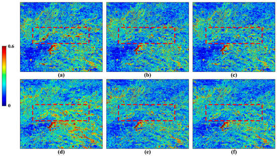
Figure 9.
Average AAD maps of the six bands between the actual image and different predictions of the DL-SDFM in the LGC site. (a) Forward prediction based on . (b) Forward prediction based on . (c) Fusion results of forward prediction. (d) Backward prediction based on . (e) Backward prediction based on . (f) Fusion results of backward prediction.
Table 3.
Quantitative results of forward predictions based on (Phe-1), forward prediction based on (Lan-1), backward prediction based on (Phe-2), backward prediction based on in (Lan-2), fusion results of forward prediction (Fus-1), and fusion results of backward prediction (Fus-2) in DL-SDFM, applied to the LGC site, where bold indicates the best result.
(3) Effectiveness of the reconstruction of the spatial detail
As shown in Figure 10, for the LGC site, both the nonlinear mapping and the super-resolution in STFDCNN fail to reconstruct the spatial details. The reconstruction of the spatial details of the predictions requires the additional high-pass modulations. The DL-SDFM, by comparison, can reconstruct the prediction with complete spatial details directly, which demonstrates its effectiveness in spatial detail reconstruction.
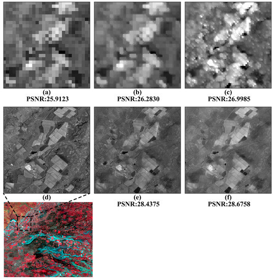
Figure 10.
Comparison of spatial details of the prediction of the STFDCNN and DL-SDFM in the LGC site. (a) Coarse image acquired at prediction date. (b) Nonlinear mapping result of STFDCNN. (c) Super-resolution result of STFDCNN. (d) Actual image acquired at prediction date. (e) Prediction of STFDCNN. (f) Prediction of DL-SDFM.
3.4.2. Prediction with Phenological Change
(1) Comparison with other fusion methods
The CI site is located in a heterogeneous rain-fed agricultural area that underwent a phenological change. As shown in Figure 11a,b, and Figure 12a, obvious phenological differences exist between the two pairs of images, increasing the difficulty of prediction. As shown in Figure 11, STARFM fails to predict the heterogeneous areas with obvious phenological changes. The zoomed-in images in Figure 11c show that the prediction of STARFM has a large spectral deviation and incomplete texture details in this area. FSDAF, by comparison, provides a prediction more similar to the actual image, while the spectral deviation is significantly reduced. STFDCNN again provides plausible spatial details; however, more obvious phenological deviation than that of the FSDAF can be seen.
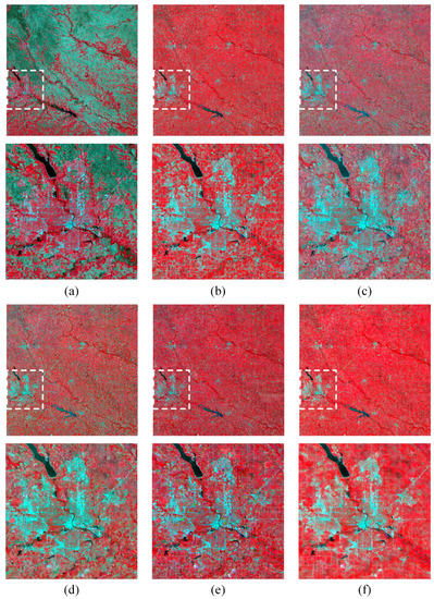
Figure 11.
Comparison of the predicted and actual images at the CI site with land-cover change. (a) Prior Landsat image acquired on 14 May 2002. (b) Actual Landsat image acquired on 2 July 2002. (c) Prediction result of STARFM. (d) Prediction result of FSDAF. (e) Prediction result of STFDCNN. (f) Prediction result of DL-SDFM.
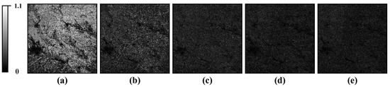
Figure 12.
Average AAD maps of the six bands between the actual image and prediction results in the CI site. (a) Actual image and prior Landsat image acquired on 14 May 2002. (b) Actual image and STARFM prediction. (c) Actual image and FSDAF prediction. (d) Actual image and STFDCNN prediction. (e) Actual image and DL-SDFM predictions.
The DL-SDFM, by contrast, yielded the prediction most similar to the actual image, suggesting that by considering the physical temporal change information, DL-SDFM is more powerful in predicting phenological change. The average AAD maps of the different fusion methods in the CI site (Figure 12) show that the prediction of the DL-SDFM has the least uncertainty compared to the other fusion methods, which further verifies the superiority of the DL-SDFM in predicting phenological change in heterogeneous areas. Quantitative results of the different fusion methods (Table 4) show that DL-SDFM also performs best with regard to metrics except in the cases of band 5 and band 7. The obvious improvement of DL-SDFM in most of the bands verifies its effectiveness in phenological change prediction.
Table 4.
Quantitative results of different fusion methods applied to the CI site. Bold indicates the best result.
(2) Effectiveness of the fusion of temporal change information with spatial information
As shown in Figure 13 and Table 5, the comparison results of the phenological change prediction, land-cover change prediction, and the combination results in the CI site are similar to those of the LGC site. The combination provides the best fusion performance for most of the bands, demonstrating the effectiveness of the weighted combination method.
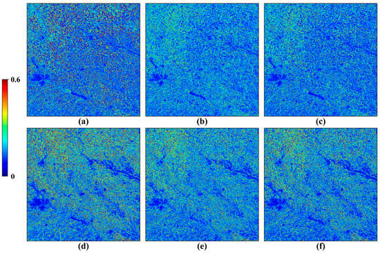
Figure 13.
The average AAD maps of the six bands between the actual image and different predictions of the DL-SDFM in CI site. (a) Forward prediction based on . (b) Forward prediction based on . (c) Fusion results of forward prediction. (d) Backward prediction based on . (e) Backward prediction based on . (f) Fusion results of backward prediction.
Table 5.
Quantitative results of forward prediction based on (Phe-1), forward prediction based on (Lan-1), backward prediction based on (Phe-2), backward prediction based on (Lan-2), fusion results of forward prediction (Fus-1), and fusion results of backward prediction (Fus-2) applied to the CI site, where bold indicates the best result.
(3) Effectiveness of the spatial detail reconstruction
The results in the CI site (Figure 14) agreed with our expectation: the nonlinear mapping and the super-resolution in STFDCNN fail to reconstruct the spatial details. The DL-SDFM, by comparison, can reconstruct the prediction with complete spatial details directly. Although the visual effect of the DL-SDFM is a bit inferior to that of the STFDCNN, the lower PSNR of the STFDCNN suggests an uncertainty accumulation during the multiple steps.
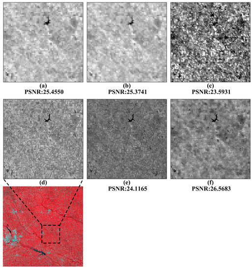
Figure 14.
Comparison of the spatial detail of the prediction of the STFDCNN and DL-SDFM in the CI site. (a) Coarse image acquired at prediction date. (b) Nonlinear mapping result of STFDCNN. (c) Super-resolution result of STFDCNN. (d) Actual image acquired at prediction date. (e) Prediction of STFDCNN. (f) Prediction of DL-SDFM.
4. Discussion
4.1. Parameter Sensitivity Analysis
The weighting parameter controls the weight of the loss of two independent mappings. In this section, we analyze the influence of in both two study sites (Figure 15). RMSE was utilized as the quantitative evaluation index of fusion performance. It can be seen that there are no significant differences in fusion accuracy under different weighting settings, indicating that the fusion performance of the DL-SDFM is not sensitive to the weighting sets. Additionally, the fusion accuracy is satisfactory when the parameter is set to 0.5, so this value was chosen in this paper.
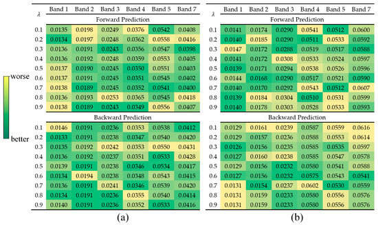
Figure 15.
Fusion performance (RMSE) for values of in DL-SDFM. (a) LGC site. (b) CI site.
We analyze the convergence of the network in two study areas. As shown in Figure 16, during the optimization, the MSE of all the bands varies significantly in the beginning; then, it falls steadily and stabilizes. The loss curves in the two study sites demonstrate that the network converges within 60 epochs.
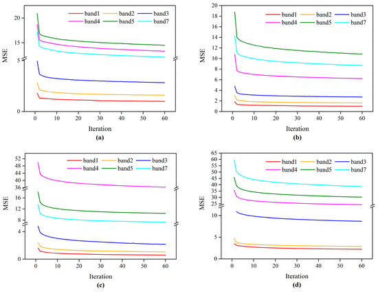
Figure 16.
Loss curves for the two study sites. (a) Forward prediction in the LGC site. (b) Backward prediction in the LGC site. (c) Forward prediction in the CI site. (d) Backward prediction in the CI site.
4.2. Advantages of the Proposed Method
The experimental results in the data sets with phenological and land-cover change verified the superiority of the DL-SDFM method over three state-of-the-art spatiotemporal fusion methods. The novelty of the DL-SDFM can be summarized as follows.
First, DL-SDFM addresses the prediction of both phenological and land-cover change with better generalization ability and robustness. The experimental results of the LGC site show that although STARFM is applicable in phenological change prediction, it fails to handle images with obvious land-cover change due to the inappropriate assumption that land cover remains unchanged. DL-SDFM, by comparison, shows a significant improvement in fusion performance, showing its effectiveness in the prediction of heterogeneous areas with phenological change. This improvement can be attributed to the temporal change-based mapping, which is learned by the two-stream CNN and has more powerful generalization ability and robustness than the traditional linear-based spatiotemporal fusion method, whose effectiveness depends on an artificial predefined weight function. DL-SDFM learns weights self-adaptively using the prior information, resulting in a more wide generality of the weight. Additionally, compared to the FSDAF, the recently proposed hybrid spatiotemporal fusion method, which is effective in land-cover change prediction due to the residual compensation, especially for the edges between two land-cover types, DL-SDFM also shows better fusion performance, which further demonstrates its ability to predict land-cover change.
Second, DL-SDFM endows the learning-based spatiotemporal fusion method with temporal change information, resulting in a more powerful ability to predict phenological change. Existing learning-based spatiotemporal fusion methods regard spatiotemporal fusion as a single image super-resolution task, which has advantages for the prediction of land-cover change. However, the lack of physical temporal change information renders these methods ineffective for the prediction of phenological change. For this reason, physical temporal change information was employed through formulating the temporal change-based mapping in DL-SDFM. Experimental results in the CI site show that although the STFDCNN provides plausible spatial details, more obvious phenological deviation than with FSDAF is observed because no physical temporal change information has been taken into account to address the phenological change. The DL-SDFM, by comparison, yields the prediction most similar to the actual image, which demonstrates its more powerful ability to predict phenological changes than the STFDCNN.
Third, DL-SDFM can directly reconstruct the prediction with complete spatial details; there is no need to use any other auxiliary modulation. Since the magnification factor of spatiotemporal fusion is much more significant than that in single-image super-resolution, existing learning-based spatiotemporal fusion methods using single-image super-resolution usually utilize the additional high-pass modulation to recover spatial details indirectly, which is tedious and increases the risk of cumulative uncertainties. The spatial information-based mapping in the DL-SDFM, by comparison, can reconstruct spatial details directly by incorporating the high-frequency information. This improvement simplifies the process of the learning-based spatiotemporal fusion method and improve the practicability.
4.3. Adaptability of the Proposed Method
In this paper, two pairs of fine and coarse image are utilized under the assumption that only two pairs of cloud-free fine and coarse image are available. This assumption is consistent with that of some typical spatiotemporal fusion methods [8,26,30], and it is considered to be reasonable, because it is usually not easy to collect more available images due to the cloud contamination and the limitations of the revisit period. For the case of more than two available pairs of fine and coarse image, it is recommended to use all the available pairs of fine and coarse image to train the two-stream CNN. Once the network has been trained, it can be directly used for the entire dataset. Meanwhile, due to the increase of the number of training samples, the robustness and generalization ability of the network will be improved.
Although in the DL-SDFM a relatively light-weight network is utilized, its computational efficiency is a bit lower than the traditional linear-based fusion methods. The average training time of each band for forward and backward prediction was 7012.8 s and 16,087.6 s, respectively. The average prediction time of each band for the above predictions was 1028.6 s and 2779.3 s. Therefore, to further improve the efficiency, it is recommended to employ GPU equipment with higher performance.
Spatiotemporal fusion methods assume that high spatial and temporal resolution images have similar spectral and radiometric properties. Since MODIS has similar bandwidth and radiation to Landsat, these two kinds of sensors were utilized to obtain the dataset used in this paper. To further apply the DL-SDFM to other types of sensors with significant radiometric inconsistency, such as the Chinese GF-1 wide-field view and MODIS [47,48], it is recommended to reduce the radiation differences first by applying a radiometric normalization.
4.4. Limitations and Future Work
DL-SDFM still has some limitations.
First, DL-SDFM requires two pairs of known fine and coarse images. However, in many regions, it is not easy to collect these images because of cloud contamination and the limitation of the revisit period. Our future work might focus on combining the deep learning-based and the linear-based spatiotemporal fusion methods to develop a hybrid spatiotemporal fusion method that is applicable in the case of one known pair of fine and coarse images. In particular, since the two mappings in DL-SDFM cannot be learned using one pair of fine and coarse images, the linear-based spatiotemporal fusion method and the deep learning-based super-resolution can be employed to address the phenological change prediction and the land-cover change prediction, respectively.
Second, although the DL-SDFM can reconstruct spatial details directly, its visual effect is slightly inferior to that of STFDCNN. The reason may lie in that the STFDCNN uses the additional high-pass modulation twice to reconstruct the spatial details. Additionally, MSE is considered to generate the overly smooth effect, so it may also be the reason that the visual effect of the DL-SDFM is slightly inferior to that of STFDCNN. Therefore, future work should improve the visual effect further by employing a more appropriate loss function to replace the MSE or using a combination of multiple loss functions [49,50].
5. Conclusions
In this paper, we propose a novel deep learning-based spatiotemporal data fusion method (DL-SDFM) with a two-stream CNN, which considers both forward and backward prediction to predict the target fine image. The proposed method simultaneously forms temporal change-based and spatial information-based mappings for the prediction of the phenological change and the land-cover change, respectively. In this way, the DL-SDFM addresses both the phenological change prediction and the land-cover change prediction with higher generality and robustness. The comparative experimental results for the test datasets demonstrated the superiority of the DL-SDFM over STARFM, FSDAF, and STFDCNN. Moreover, compared to the existing learning-based spatiotemporal fusion methods, the DL-SDFM has a more powerful ability to predict the phenological change, due to the introduction of the physical temporal change information. Additionally, the ability of DL-SDFM to reconstruct the prediction with complete spatial details directly simplifies the process of deep learning-based spatiotemporal fusion and improves its applicability. However, some potential limitations are worthwhile to note. Future improvements include applying the DL-SDFM to the case of one known pair of fine and coarse images and the improvement of the visual effect by employing a more appropriate loss function.
Author Contributions
Conceptualization, D.J., C.S., and C.C.; methodology, D.J.; experiments, D.J. and S.S.; analysis, D.J., L.N., and C.H.; writing, D.J.; supervision, C.C. All authors have read and agreed to the published version of the manuscript.
Funding
This research was funded by National Key Research and Development Plan of China grant number [2019YFA0606901].
Acknowledgments
We would like to thank the high-performance computing support from the Center for Geodata and Analysis, Faculty of Geographical Science, Beijing Normal University [https://gda.bnu.edu.cn/].
Conflicts of Interest
The authors declare no conflict of interest.
References
- Suess, S.; van der Linden, S.; Okujeni, A.; Griffiths, P.; Leitão, P.J.; Schwieder, M.; Hostert, P. Characterizing 32 years of shrub cover dynamics in southern Portugal using annual Landsat composites and machine learning regression modeling. Remote Sens. Environ. 2018, 219, 353–364. [Google Scholar] [CrossRef]
- Arévalo, P.; Olofsson, P.; Woodcock, C.E. Continuous monitoring of land change activities and post-disturbance dynamics from Landsat time series: A test methodology for REDD+ reporting. Remote Sens. Environ. 2019, 238, 111051. [Google Scholar] [CrossRef]
- Interdonato, R.; Ienco, D.; Gaetano, R.; Ose, K. DuPLO: A DUal view Point deep Learning architecture for time series classification. ISPRS J. Photogramm. Remote Sens. 2019, 149, 91–104. [Google Scholar] [CrossRef]
- Lees, K.J.; Quaife, T.; Artz, R.R.E.; Khomik, M.; Clark, J.M. Potential for using remote sensing to estimate carbon fluxes across northern peatlands—A review. Sci. Total Environ. 2018, 615, 857–874. [Google Scholar] [CrossRef]
- Feng, G.; Masek, J.; Schwaller, M.; Hall, F. On the blending of the Landsat and MODIS surface reflectance: Predicting daily Landsat surface reflectance. IEEE Trans. Geosci. Remote Sens. 2006, 44, 2207–2218. [Google Scholar] [CrossRef]
- Gao, F.; Hilker, T.; Zhu, X.; Anderson, M.; Masek, J.; Wang, P.; Yang, Y. Fusing Landsat and MODIS Data for Vegetation Monitoring. IEEE Geosci. Remote Sens. Mag. 2015, 3, 47–60. [Google Scholar] [CrossRef]
- Zhu, X.; Helmer, E.H.; Gao, F.; Liu, D.; Chen, J.; Lefsky, M.A. A flexible spatiotemporal method for fusing satellite images with different resolutions. Remote Sens. Environ. 2016, 172, 165–177. [Google Scholar] [CrossRef]
- Zhu, X.; Chen, J.; Gao, F.; Chen, X.; Masek, J.G. An enhanced spatial and temporal adaptive reflectance fusion model for complex heterogeneous regions. Remote Sens. Environ. 2010, 114, 2610–2623. [Google Scholar] [CrossRef]
- Emelyanova, I.V.; McVicar, T.R.; Van Niel, T.G.; Li, L.T.; van Dijk, A.I.J.M. Assessing the accuracy of blending Landsat–MODIS surface reflectances in two landscapes with contrasting spatial and temporal dynamics: A framework for algorithm selection. Remote Sens. Environ. 2013, 133, 193–209. [Google Scholar] [CrossRef]
- Wang, J.; Huang, B. A Rigorously-Weighted Spatiotemporal Fusion Model with Uncertainty Analysis. Remote Sens. 2017, 9, 990. [Google Scholar] [CrossRef]
- Cheng, Q.; Liu, H.; Shen, H.; Wu, P.; Zhang, L. A Spatial and Temporal Nonlocal Filter-Based Data Fusion Method. IEEE Trans. Geosci. Remote Sens. 2017, 55, 4476–4488. [Google Scholar] [CrossRef]
- Wang, Q.; Atkinson, P.M. Spatio-temporal fusion for daily Sentinel-2 images. Remote Sens. Environ. 2018, 204, 31–42. [Google Scholar] [CrossRef]
- Kwan, C.; Budavari, B.; Gao, F.; Zhu, X. A Hybrid Color Mapping Approach to Fusing MODIS and Landsat Images for Forward Prediction. Remote Sens. 2018, 10, 520. [Google Scholar] [CrossRef]
- Ping, B.; Meng, Y.; Su, F. An Enhanced Linear Spatio-Temporal Fusion Method for Blending Landsat and MODIS Data to Synthesize Landsat-Like Imagery. Remote Sens. 2018, 10, 881. [Google Scholar] [CrossRef]
- Senf, C.; Leitão, P.J.; Pflugmacher, D.; van der Linden, S.; Hostert, P. Mapping land cover in complex Mediterranean landscapes using Landsat: Improved classification accuracies from integrating multi-seasonal and synthetic imagery. Remote Sens. Environ. 2015, 156, 527–536. [Google Scholar] [CrossRef]
- Jia, K.; Liang, S.; Zhang, N.; Wei, X.; Gu, X.; Zhao, X.; Yao, Y.; Xie, X. Land cover classification of finer resolution remote sensing data integrating temporal features from time series coarser resolution data. ISPRS J. Photogramm. Remote Sens. 2014, 93, 49–55. [Google Scholar] [CrossRef]
- Chen, B.; Chen, L.; Huang, B.; Michishita, R.; Xu, B. Dynamic monitoring of the Poyang Lake wetland by integrating Landsat and MODIS observations. ISPRS J. Photogramm. Remote Sens. 2018, 139, 75–87. [Google Scholar] [CrossRef]
- Shen, H.; Huang, L.; Zhang, L.; Wu, P.; Zeng, C. Long-term and fine-scale satellite monitoring of the urban heat island effect by the fusion of multi-temporal and multi-sensor remote sensed data: A 26-year case study of the city of Wuhan in China. Remote Sens. Environ. 2016, 172, 109–125. [Google Scholar] [CrossRef]
- Xia, H.; Chen, Y.; Li, Y.; Quan, J. Combining kernel-driven and fusion-based methods to generate daily high-spatial-resolution land surface temperatures. Remote Sens. Environ. 2019, 224, 259–274. [Google Scholar] [CrossRef]
- Houborg, R.; McCabe, M.F.; Gao, F. A Spatio-Temporal Enhancement Method for medium resolution LAI (STEM-LAI). Int. J. Appl. Earth Obs. Geoinf. 2016, 47, 15–29. [Google Scholar] [CrossRef]
- Li, Z.; Huang, C.; Zhu, Z.; Gao, F.; Tang, H.; Xin, X.; Ding, L.; Shen, B.; Liu, J.; Chen, B.; et al. Mapping daily leaf area index at 30 m resolution over a meadow steppe area by fusing Landsat, Sentinel-2A and MODIS data. Int. J. Remote Sens. 2018, 39, 9025–9053. [Google Scholar] [CrossRef]
- Ke, Y.; Im, J.; Park, S.; Gong, H. Spatiotemporal downscaling approaches for monitoring 8-day 30m actual evapotranspiration. ISPRS J. Photogramm. Remote Sens. 2017, 126, 79–93. [Google Scholar] [CrossRef]
- Ma, Y.; Liu, S.; Song, L.; Xu, Z.; Liu, Y.; Xu, T.; Zhu, Z. Estimation of daily evapotranspiration and irrigation water efficiency at a Landsat-like scale for an arid irrigation area using multi-source remote sensing data. Remote Sens. Environ. 2018, 216, 715–734. [Google Scholar] [CrossRef]
- Zhu, X.; Cai, F.; Tian, J.; Williams, K.T. Spatiotemporal Fusion of Multisource Remote Sensing Data: Literature Survey, Taxonomy, Principles, Applications, and Future Directions. Remote Sens. 2018, 10, 527. [Google Scholar] [CrossRef]
- Zhang, H.K.; Huang, B.; Zhang, M.; Cao, K.; Yu, L. A generalization of spatial and temporal fusion methods for remotely sensed surface parameters. Int. J. Remote Sens. 2015, 36, 4411–4445. [Google Scholar] [CrossRef]
- Huang, B.; Song, H. Spatiotemporal Reflectance Fusion via Sparse Representation. IEEE Trans. Geosci. Remote Sens. 2012, 50, 3707–3716. [Google Scholar] [CrossRef]
- Song, H.; Huang, B. Spatiotemporal Satellite Image Fusion Through One-Pair Image Learning. IEEE Trans. Geosci. Remote Sens. 2013, 51, 1883–1896. [Google Scholar] [CrossRef]
- Wu, B.; Huang, B.; Zhang, L. An Error-Bound-Regularized Sparse Coding for Spatiotemporal Reflectance Fusion. IEEE Trans. Geosci. Remote Sens. 2015, 53, 6791–6803. [Google Scholar] [CrossRef]
- Wei, J.; Wang, L.; Liu, P.; Song, W. Spatiotemporal Fusion of Remote Sensing Images with Structural Sparsity and Semi-Coupled Dictionary Learning. Remote Sens. 2017, 9, 21. [Google Scholar] [CrossRef]
- Wei, J.; Wang, L.; Liu, P.; Chen, X.; Li, W.; Zomaya, A.Y. Spatiotemporal Fusion of MODIS and Landsat-7 Reflectance Images via Compressed Sensing. IEEE Trans. Geosci. Remote Sens. 2017, 55, 7126–7139. [Google Scholar] [CrossRef]
- Liu, X.; Deng, C.; Wang, S.; Huang, G.; Zhao, B.; Lauren, P. Fast and Accurate Spatiotemporal Fusion Based Upon Extreme Learning Machine. IEEE Geosci. Remote Sens. Lett. 2016, 13, 2039–2043. [Google Scholar] [CrossRef]
- Tan, Z.; Yue, P.; Di, L.; Tang, J. Deriving High Spatiotemporal Remote Sensing Images Using Deep Convolutional Network. Remote Sens. 2018, 10, 1066. [Google Scholar] [CrossRef]
- Song, H.; Liu, Q.; Wang, G.; Hang, R.; Huang, B. Spatiotemporal Satellite Image Fusion Using Deep Convolutional Neural Networks. IEEE J. Sel. Top. Appl. Earth Obs. 2018, 11, 821–829. [Google Scholar] [CrossRef]
- Szegedy, C.; Wei, L.; Yangqing, J.; Sermanet, P.; Reed, S.; Anguelov, D.; Erhan, D.; Vanhoucke, V.; Rabinovich, A. Going deeper with convolutions. In Proceedings of the 2015 IEEE Conference on Computer Vision and Pattern Recognition (CVPR), Boston, MA, USA, 7–12 June 2015; pp. 1–9. [Google Scholar]
- Yuan, Q.; Wei, Y.; Meng, X.; Shen, H.; Zhang, L. A Multiscale and Multidepth Convolutional Neural Network for Remote Sensing Imagery Pan-Sharpening. IEEE J. Sel. Top. Appl. Earth Obs. 2018, 11, 978–989. [Google Scholar] [CrossRef]
- Zhang, Q.; Yuan, Q.; Zeng, C.; Li, X.; Wei, Y. Missing Data Reconstruction in Remote Sensing Image With a Unified Spatial–Temporal–Spectral Deep Convolutional Neural Network. IEEE Trans. Geosci. Remote Sens. 2018, 56, 4274–4288. [Google Scholar] [CrossRef]
- Zhang, Q.; Yuan, Q.; Li, J.; Yang, Z.; Ma, X. Learning a Dilated Residual Network for SAR Image Despeckling. Remote Sens. 2018, 10, 196. [Google Scholar] [CrossRef]
- Shi, W.; Jiang, F.; Zhao, D. Single image super-resolution with dilated convolution based multi-scale information learning inception module. In Proceedings of the 2017 IEEE International Conference on Image Processing (ICIP), Beijing, China, 17–20 September 2017; pp. 977–981. [Google Scholar]
- Wang, P.; Chen, P.; Yuan, Y.; Liu, D.; Huang, Z.; Hou, X.; Cottrell, G. Understanding Convolution for Semantic Segmentation. In Proceedings of the 2018 IEEE Winter Conference on Applications of Computer Vision (WACV), Lake Tahoe, NV, USA, 12–15 March 2018; pp. 1451–1460. [Google Scholar]
- Kingma, D.; Ba, J. Adam: A Method for Stochastic Optimization. arXiv 2014, arXiv:1412.6980. [Google Scholar]
- Yuan, Q.; Zhang, Q.; Li, J.; Shen, H.; Zhang, L. Hyperspectral Image Denoising Employing a Spatial–Spectral Deep Residual Convolutional Neural Network. IEEE Trans. Geosci. Remote Sens. 2019, 57, 1205–1218. [Google Scholar] [CrossRef]
- Zhou, W.; Bovik, A.C. A universal image quality index. IEEE Signal Process. Lett. 2002, 9, 81–84. [Google Scholar] [CrossRef]
- Zhou, W.; Bovik, A.C.; Sheikh, H.R.; Simoncelli, E.P. Image quality assessment: From error visibility to structural similarity. IEEE Trans. Image Process. 2004, 13, 600–612. [Google Scholar] [CrossRef]
- Khan, M.M.; Alparone, L.; Chanussot, J. Pansharpening Quality Assessment Using the Modulation Transfer Functions of Instruments. IEEE Trans. Geosci. Remote Sens. 2009, 47, 3880–3891. [Google Scholar] [CrossRef]
- Yuhas, R.H.; Goetz, A.F.H.; Boardman, J.W. Discrimination among semi-arid landscape endmembers using the Spectral Angle Mapper (SAM) algorithm. In Proceedings of the Annual JPL Airborne Earth Science Workshop, Pasadena, CA, USA, 1–5 June 1992; pp. 147–149. [Google Scholar]
- Sheikh, H.R.; Sabir, M.F.; Bovik, A.C. A Statistical Evaluation of Recent Full Reference Image Quality Assessment Algorithms. IEEE Trans. Image Process. 2006, 15, 3440–3451. [Google Scholar] [CrossRef] [PubMed]
- Tao, G.; Jia, K.; Zhao, X.; Wei, X.; Xie, X.; Zhang, X.; Wang, B.; Yao, Y.; Zhang, X. Generating High Spatio-Temporal Resolution Fractional Vegetation Cover by Fusing GF-1 WFV and MODIS Data. Remote Sens. 2019, 11, 2324. [Google Scholar] [CrossRef]
- Cui, J.; Zhang, X.; Luo, M. Combining Linear Pixel Unmixing and STARFM for Spatiotemporal Fusion of Gaofen-1 Wide Field of View Imagery and MODIS Imagery. Remote Sens. 2018, 10, 1047. [Google Scholar] [CrossRef]
- Ledig, C.; Theis, L.; Huszár, F.; Caballero, J.; Cunningham, A.; Acosta, A.; Aitken, A.; Tejani, A.; Totz, J.; Wang, Z.; et al. Photo-Realistic Single Image Super-Resolution Using a Generative Adversarial Network. In Proceedings of the 2017 IEEE Conference on Computer Vision and Pattern Recognition (CVPR), Honolulu, HI, USA, 21–26 July 2017; pp. 105–114. [Google Scholar]
- Tan, Z.; Di, L.; Zhang, M.; Guo, L.; Gao, M. An Enhanced Deep Convolutional Model for Spatiotemporal Image Fusion. Remote Sens. 2019, 11, 2898. [Google Scholar] [CrossRef]


© 2020 by the authors. Licensee MDPI, Basel, Switzerland. This article is an open access article distributed under the terms and conditions of the Creative Commons Attribution (CC BY) license (http://creativecommons.org/licenses/by/4.0/).