Article

Identifying the Contributions of Multi-Source Data for Winter Wheat Yield Prediction in China

1
State Key Laboratory of Earth Surface Processes and Resource Ecology/MEM&MoE Key Laboratory of Environmental Change and Natural Hazards, Faculty of Geographical Science, Beijing Normal University; Beijing 100875, China
2
Key Laboratory of Land Surface Pattern and Simulation, Institute of Geographical Sciences and Natural Resources Research, Chinese Academy of Sciences, Beijing 100101, China
3
Natural Resources Institute Finland (Luke), FI-00790 Helsinki, Finland
*
Author to whom correspondence should be addressed.
Remote Sens. 2020, 12(5), 750; https://doi.org/10.3390/rs12050750
Submission received: 29 January 2020 / Revised: 20 February 2020 / Accepted: 23 February 2020 / Published: 25 February 2020

Abstract

:
Wheat is a leading cereal grain throughout the world. Timely and reliable wheat yield prediction at a large scale is essential for the agricultural supply chain and global food security, especially in China as an important wheat producing and consuming country. The conventional approach using either climate or satellite data or both to build empirical and crop models has prevailed for decades. However, to what extent climate and satellite data can improve yield prediction is still unknown. In addition, socio-economic (SC) factors may also improve crop yield prediction, but their contributions need in-depth investigation, especially in regions with good irrigation conditions, sufficient fertilization, and pesticide application. Here, we performed the first attempt to predict wheat yield across China from 2001 to 2015 at the county-level by integrating multi-source data, including monthly climate data, satellite data (i.e., Vegetation indices (VIs)), and SC factors. The results show that incorporating all the datasets by using three machine learning methods (Ridge Regression (RR), Random Forest (RF), and Light Gradient Boosting (LightGBM)) can achieve the best performance in yield prediction (R2: 0.68~0.75), with the most individual contributions from climate (~0.53), followed by VIs (~0.45), and SC factors (~0.30). In addition, the combinations of VIs and climate data can capture inter-annual yield variability more effectively than other combinations (e.g., combinations of climate and SC, and combinations of VIs and SC), while combining SC with climate data can better capture spatial yield variability than others. Climate data can provide extra and unique information across the entire growing season, while the peak stage of VIs (Mar.~Apr.) do so. Furthermore, incorporating spatial information and soil proprieties into the benchmark models can improve wheat yield prediction by 0.06 and 0.12, respectively. The optimal wheat prediction can be achieved with approximately a two-month leading time before maturity. Our study develops timely and robust methods for winter wheat yield prediction at a large scale in China, which can be applied to other crops and regions.

Graphical Abstract

1. Introduction

Wheat (Triticum aestivum L.) is the leading cereal grain in the world, providing the most calories and protein for world food supply [1,2]. China is the major wheat producing and consuming country globally [3,4,5,6], with winter wheat reaching about 85% of its total summer grain production [7]. Wheat yield in China, however, has stagnated in recent years [7,8]. Timely and reliable crop yield prediction has increasingly become one of the key issues for food security, supply chain planning of agriculture industry, and market prediction for the entire population [9,10]. Furthermore, such yield estimations will also help farmers to make informed management and financial decisions in advance [11,12]. In recent years, extensive studies have focused on crop yield prediction at different spatial scales by either using statistical regression models or crop models in various countries [13,14,15,16]. With some explicit cause-effect relationships [7,8], regression models have been increasingly replaced by crop models due to their lower required explanation and limited spatial generalization in recent years [17]. However, there are still many problems regarding crop models since they over-depend on extensive input data such as climate, cultivar, management, and soil conditions, as well as huge requirements in replicability, transparency, and code efficiency [1,16,18]. Thus, the problems associated with the above two methods highlight the need for another novel approach with an ability to provide timely, reliable, and cost-effective wheat yield prediction.
Machine learning (ML) has been widely and successfully applied in various data-driven fields, such as for analysis of landslides susceptibility, image processing, and facial expression recognition [19,20,21,22,23,24], as well as in various agricultural fields such as crop classification [25,26], grassland fuel content estimation [27], and crop yield estimation [28,29]. Compared with crop models and the traditional statistical methods, ML has limited process-based interpretation and can handle nonlinear relationships for crop yield prediction. Several previous studies had proved its ability in improving crop yield prediction [1,12,28,30,31,32,33]. However, such methods have rarely been tested for crop yield prediction in China.
Crop yields are affected by many variables, which are generally classified into dynamic and static variables. Climate, vegetation indices (VIs), and social-economic (SC) factors belong to the former, which can be monitored at various temporal scales [1,34]. Climate and VIs are usually available through observation stations or remote sensing, while SC factors are reported in annual statistic reports of different administrative units [8,18]. Variables unchanged during the growing season are the static ones, including spatial information (e.g., latitude and longitude) and soil features. Distinct spatial patterns of crop yields have substantiated strongly that these static variables have impacts on final yields [1,35,36], implying their potential roles in improving wheat yield estimation and gap analysis [37].
Satellite remote sensing has been successfully used for monitoring crop growth, tillage differentiation, and yield prediction owing to spatiotemporal capture of earth’s surface across various spectral bands [38]. Among them, visible and near-infrared data have the most advantages in monitoring crop growth for estimating crop yield by developing various vegetation indices [38,39,40,41]. Since Tucker et al. (1980) developed the first Normalized Difference Vegetation Index (NDVI) [42], several popular VIs have been extensively applied in the agricultural field (e.g., NDVI, enhanced vegetation index (EVI), green chlorophyll vegetation index (GCVI)) [18,25,40]. Given the spectral indices can dynamically capture crop growing conditions through various combinations, and these various products have commonly shared and complementary information to contribute to yield prediction, we focused on three VIs associated strongly with yield: EVI, GCVI, and NDVI, to determine their contributions to wheat yield prediction in China [43,44,45,46]. In addition, climate variables (e.g., temperature and precipitation) are the primary inputs for crop yield prediction, which can capture the environment information [1,34].
With exception of dynamic variables (e.g., VIs, climate data) monitoring natural environment states, SC factors also play an important role in crop yield and production [47,48], especially irrigation, fertilizer application, pesticide use, farm mechanization status, and others. For example, adopting the best farm management practices could increase crop yield [49,50]. Understanding how changes in farm management practices can benefit crop yield prediction, especially for spatial analyses of yield [47,49]. However, very few studies have considered the contribution of SC factors for crop yield prediction at a regional scale so far.
Although the availability and accessibility of multi-source data with potentially valuable information for agricultural applications increase, very few studies have quantified their shared and unique contributions to predicting wheat yields and their spatiotemporal variations across China. Therefore, we first adopt exploratory data analysis (EDA) to select variables that are significantly related to crop yield. Then a multiple linear regression [ridge regression (RR)] and two machine learning methods—Random Forest (RF) and Light Gradient Boosting (LightGBM)—are applied to estimate wheat yield and compare their yield prediction performance by using different combinations of input variables with different growing stages. In this paper, the following questions need to be solved: (1) how can we integrate such multi-source data (climate, satellite, and SC factors) to derive the best wheat yield prediction model to explain the spatio-temporal variation of yields? (2) how much will such unique and shared information from temporal dynamic data improve wheat yield prediction across China? (3) how do ML techniques perform compared with the common regression technique for crop yield prediction? (4) to what degrees will the static variables (spatial information and soil properties) improve wheat yield prediction in China?

2. Material and Methods

2.1. Study Area

In this study, the main winter wheat producing areas in China—North China Plain (NCP) (Figure 1) was selected as our research study, which covers 398 counties in five provinces (Hebei, Shandong, Henan, Jiangsu, and Anhui). This region, between 29°41′N~42°40′N and 111°21′E ~ 122°43′E, is one of the important food baskets in China, with a total wheat cultivation area of 16.18 × 10⁴ ha, accounting for 67.02% of the total wheat area and 75.79% of the total wheat yield in China [17,51]. The region mainly has a semi-humid climate, with the total annual precipitation from 400 to 800 mm, and the total amount is relatively low for winter wheat growth. Therefore, the abundance and shortage of water resources greatly affects winter wheat yield, and the social and economic development factors (e.g., agricultural irrigation, fertilizer, and pesticide consumption) play a great role in crop yield [17,51]. Winter wheat grown across this region is generally sown at the beginning of October (spring) and harvested at the end of May or the beginning of June (autumn) in the following year [17].

2.2. Dataset and Preprocessing

The yield records, cropping area, climate, SC, and satellite variables were obtained from various sources (Table 1). We first unified spatial and temporal resolutions of climate and satellite data into 1 km and monthly interval, respectively. Then crop maps were used to mask climate and satellite data, and aggregate mean monthly variables at the county-level.

2.2.1. Crop Yield and Area

The winter wheat yields at county-level were obtained from the Agricultural Yearbook of each county (http://www.stats.gov.cn) from 2001 to 2015 (unit: kg/ha). A preliminary data quality check was conducted to identify and filter the outliers: (i) those that fell outside the range of biophysical attainable yield records. (ii) those that fell outside the range of the mean from 2001 to 2015 plus or minus two times of standard deviation [17,52,53]. Furthermore, the accurate information of annual winter wheat regions is vital to predicting yield, but is not available in the public domain. The National Land Cover Dataset (NLCD) of China, with a spatial resolution of 1 km for 2005, 2010, and 2015, was provided by Data Center for Resources and Environmental Sciences, Chinese Academy of Sciences (http://www.resdc.cn/). These datasets are generated by visual interpretation and digitization of Landsat TM/ETM+ images with an overall classification accuracy above 90% [54,55]. The typical cropping system of this region is a winter wheat-summer maize rotation system, and only wheat is sown in dryland during our study period [7,8]. Therefore, we extract dryland in cultivated land as the winter wheat areas in the three time periods and then use the three generated area maps as the broad wheat cropping areas (Figure 1). According to the statistical data from Agricultural Yearbook of each province (Figure A1), we assume that there is no significant crop area change in the five years. Therefore, the crop coverage map of 2005 was used to mask the explanatory variables (i.e., climate, satellite data, and soil properties) for 2001-2005, 2010 for 2005-2010, and 2015 for 2010-2015, respectively.

2.2.2. Satellite Data

Moderate Resolution Imaging Spectroradiometer (MODIS) Terra MOD09A1 Version 6 with 500 m and 8-day resolution (https://doi.org/10.5067/MODIS/MOD09A1.006) from 2000 to 2015 were retrieved from GEE (Google Earth Engine) platform. The GEE platform hosts remotely sensed imagery and other data that are freely available. NDVI is the widest indicator to monitor crop growth and predict yield since the early 1980s [42,56], which is highly correlated with the vegetation vigor and canopy background variations [46]. EVI can improve sensitivity in high biomass regions and indicate a potential photosynthetic capacity due to its usefulness in estimating the fraction of absorbed photosynthetically active radiation (fPAR) related to chlorophyll contents [44]. GCVI has been found to have the most significant linear relationship with the leaf area index (LAI) compared with other VIs [43,45]. Therefore, we chose three commonly used VIs—NDVI [42], EVI [44], and GCVI [43] to approximate aboveground vegetation dynamics associated with biomass and photosynthesis. The three indexes were calculated as
NDVI = (NIR − RED)/(NIR + RED),
GCVI = (NIR/GREEN) − 1,
EVI = G × (NIR − RED)/(NIR + C1 × RED − C2 × BLUE + L),
where NIR, RED, GREEN, and BLUE represent reflectance at near infrared, red, green, and blue wavelengths, respectively. Here, the values of coefficients for EVI were set at G = 2, C1 = 6, C2 = 7.5, and L = 1.

2.2.3. Climate Data

Meteorological forcing data were obtained from the TerraClimate dataset (http://doi.org/10.7923/G43J3B0R) within the GEE platform. This monthly dataset generated from climatological aided interpolation, with a high spatial resolution (1/24°, ~4 km) for global terrestrial surfaces from 1958–2018, was produced by Abatzoglou et al., (2018). Compared with the Climatic Research Unit (CRU) and other coarser resolution gridded datasets, TerraClimate data showed significant improvements in the overall mean absolute error and increased spatial realism over maximum (Tmax), minimum temperatures (Tmin), precipitation (Pre), vapor pressure (Vap), and other variables [57].

2.2.4. Socio-Economic Factor

Except for climate and satellite data, socio-economic features could also improve winter wheat yield prediction, especially in the NCP. Winter wheat in this region is generally grown under non-limiting conditions, with sufficient irrigation, and fertilizer applications [51]. Therefore, the irrigation area (IA; unit: ha), the consumption of chemical fertilizers (CCF, unit: ton), the consumption of agricultural pesticide (CAP, unit: ton), the total power of agricultural machinery (TPAM, unit: kw), and the electricity consumed in rural areas (ECRA, unit: kwh) at the county-level were obtained from the Agricultural Yearbook of each county (http://www.stats.gov.cn) from 2001 to 2015 to assess the influence of socio-economic factors on yield prediction.

2.2.5. Other Datasets

The DEM (digital elevation model) with 90 m × 90 m was obtained from the Shuttle Radar Topography Mission (SRTM) digital elevation dataset. Soil properties [58] including soil depth, soil texture, organic carbon content, pH, cation exchange capacity, and bulk density for the topsoil layer (0–30 cm) and the subsoil layer (30–100 cm) at 0.00833° (~1 km) were also collected, which were gathered from a soil particle-size distribution dataset in China (http://globalechange.bnu.edu.cn).

2.3. Methods

Two high-performance-based machine-learning methods (RF and LightGBM) and a traditional multiple regression method (RR) were applied to winter wheat prediction in the NCP. First, all the variables and yields from 2001 to 2015 were normalized to have mean zero and unit standard deviation. Therefore, all of the variables in the models are at a common level and are comparable [34]. Second, the whole dataset across all years and counties were randomly divided into two parts: training (70%) and testing (30%) datasets. Then, the cross-validated R2 was calculated by applying 10-fold cross-validation and GridSearchCV packages in Python 3.7 to optimize hyper-parameters for each method from empirical candidates only using the training data [1]. Finally, we employed the three optimized models on the testing dataset and calculated the predicted R2. In order to minimize the uncertainty of R2, the whole process for one predicted R2 was repeated 100 times to calculate the mean predicted R2, which was used to evaluate the performance of different models. All the R2 in the following sections refer to the mean predicted R2. The results of those models were utilized to compare with each other. Here, Python 3.7 was applied to develop the three models. The following sections describe the three methods in details.

2.3.1. Ridge Regression (RR)

RR is one of the most popular multiple linear regression methods proposed by Hoerl and Kennard (1970). Compared with other linear regression methods, this algorithm introduces a method for showing in two dimensions the effects of nonorthogonality, namely ridge trace [59], which locates the minimum residual sum of squares of the prediction and limits the sum of squares of the regression coefficients [60,61]. The alpha (Regularization strength) is the main hyper-parameter that needs to be tuned. RR method is mainly applied to multiple regression data with high correlations. When correlation occurs, least squares estimates are unbiased, but their variances are large so they may be far from the true value. By adding a degree of bias to the regression estimates, RR can reduce the standard errors. Thus, the RR performs well and results in parsimonious models. Since the input variables (i.e., climate and VIs in different months) have correlations, it is rational to use the RR model for predicting yield.

2.3.2. Random Forest (RF)

RF, first developed by Breiman (2001), is an ensemble learning method, which creates many regression trees that are generated by a large set of decision trees for computing regression [62]. The RF algorithm has been applied to research as a powerful tool for yield prediction [1,33]. Each in the RF algorithm increases diversity among the regression trees by selecting a random set of variables and samples of the dataset over the different tree induction processes [63]. The number of trees in the forest, the tree number of predictive variables used to split the nodes, and the maximum depth of tree are three user-defined hyper-parameters that needed to be tuned [1]. The RF usually performs overall better and is more accurate than any of decision tree [63], as the bias is compensated for by the single decision tree due to the randomness. Furthermore, RF can effectively deal with high-dimensional datasets [1], which can analyze these datasets, in our research (e.g., five monthly climate variables and three monthly indices derived from the satellite data over seven months).

2.3.3. Light Gradient Boosting Machine (LightGBM)

The LightGBM, generated by Ke and colleagues in 2017, is a relatively new machine learning method, which is also an ensemble learning method and is mainly based on the Decision Tree algorithm [64]. This method has been applied to many different kinds of data mining tasks (e.g., classification, regression, and ordering) and exhibits excellent accuracy [65]. The LightGBM algorithm contains two novel techniques: the gradient-based one-side sampling and the exclusive feature bundling, respectively, which are convenient for dealing with a number of data instances and a number of features. Therefore, compared with other similar algorithms (e.g., eXtreme Gradient Boosting) [66], LightGBM can significantly perform better in terms of computational speed and memory consumption. The number of leaves per tree, the speed of iteration, the maximum depth of the tree, the minimum number of the records for a leaf, the fraction of features selected randomly in each iteration, and the fraction of data to be used for each iteration are the main parameters that needed to be tuned in the LightGBM algorithm [66].

2.4. Experiment Design

Three experiments were designed to identify the contribution of multi-source data to improving wheat yield prediction and answer the four questions by using RR, RF, and LightGBM mentioned above. The details about those experiments are shown in the following sections.

2.4.1. The First Experiment to Separate the Spatial and Temporal Variations of Yields and Combine the Explanatory Ones Differently

To distinctly capture the spatial and temporal patterns, three options for yield were performed (Figure 2). Option 1: all recorded yields and input variables were selected in a county as a sample, namely “Raw”. Such raw yield essentially includes both spatial and temporal features of yield variability. Option 2: Linear trends of the raw yield and input variables at the county level (i.e., detrend) were removed. Then we obtained the corresponding detrended datasets, namely “Detrend”, which thus removed their spatial variabilities at the county-level while the remaining temporal variabilities remained both in yield and input variables when compared with raw values [34]. Comparing the results between Option 1 and 2 can reveal their distinctions in explaining spatial and temporal variability. Option 3: Using the average of the raw data covering 2001-2015 for each county plus the “Detrend” (Option 2) to obtain another new dataset, namely “Detrend+Mean”. It maintains the spatial variability when compared with the “Detrend” dataset, but removes the multi-year linear trend when compared with the raw one [34].
Based on the three dynamic datasets included as explanatory variables (climate, satellite, and SC factors), seven different combinations were applied to develop the models: (1) SC only; (2) VIs only; (3) Climate only; (4) SC combined with VIs; (5) SC combined with climate; (6) VI combined with climate; (7) SC combined with VIs and climate. Therefore, a total of 21 (3 × 7) experiments were conducted. Through comparing the prediction R2 of the above seven inputs and three types of yield data, we tried to investigate which combination and which method perform the best in explaining the temporal and spatial patterns of yield variability at the county-level.

2.4.2. The Second Experiment to Quantify the Contributions of Time Series Data to Yield Prediction

The first sub-group experiment is designed to investigate how climate and VIs during different growing stages—separated by early (Oct.–Feb.: the emergence to green-up period), peak (Mar. –Apr.: the green-up to heading period) and late (May–Jun.: the heading to maturity period) stages [51]—contribute to yield prediction (the second question). Then to evaluate the influence of climate and VIs from different growing stages on crop yield estimation, VIs (climate) data from the whole growing season but only the climate (satellite) data during one specific growing stage in the following six options WERE used. Option 1: only using climate data during the early growing stage (“early climate + all VIs data”); Option 2: only using climate data during the peak growing stage (“peak climate +all VIs data”); Option 3: only using climate data during the late growing stage (“late climate +all VIs data”). Option 4: only using satellite data during the early growing stage (“early VIs + all climate data”); Option 5: only using satellite data during the peak growing stage (“peak VIs + all climate data”); Option 6: only using satellite data during the late growing stage (“late VIs + all climate data”). The predicted R2 values of the new models were compared with the corresponding benchmark and determined climate (VIs), at which stage we could have more additional contributions to the final yield prediction.
The second sub-group experiment was focused on the temporal progress of the model performance after inserting another monthly variable. For any month during the growing season, the input information from the current month and all previous months since the beginning of the growing season was used to predict the final wheat yield. The predicted R2 from different models based on different combinations of inputs (i.e., climate data only, VIs data only, and all data combined) were obtained and compared to quantify the added values of either climate data or VIs data over the time for final wheat yield prediction.

2.4.3. The Third Experiment to Investigate the Values of Static Variables on Yield Prediction, and to Validate the Model Performances

The third experiment was designed to determine whether adding spatial and soil proprieties information can improve the performance of wheat yield prediction. There were three static spatial information variables (DEM, latitude, and longitude) and 14 soil proprieties (topsoil and the subsoil layer) in the following two options: Option 1: only adding spatial information (“With spatial features”), Option 2: only adding soil features (“With soil features”). Their predicted R2 with those of benchmark models (Option 3) was compared and investigated to obtain the additional values of spatial and soil features for predicting wheat yield.
Finally, the “leave-one-year-out” validation was performed from 2001–2015 to assess the generalization ability of those models. Specifically, One-year data were used for testing and all the other years for training. For example, the 2001-2014 data were chosen as training data to predict the crop yield in 2015, and the data for 2001–2013 and 2015 were applied as training data to predict the crop yield for 2014.

3. Results

3.1. Exploratory Data Analysis (EDA)

The correlations between the variables and wheat yields were conducted by using the 2001–2015 raw data (Table 2). The results show that all variables are significantly correlated with yield (p < 0.01), hence they would be included to develop yield models. Tmax (0.03) and Tmin (−0.08) are negatively and positively correlated with yields, respectively. However, a negative correlation (−0.4) is found between Pre and Yield, suggesting that good irrigation conditions in the NCP should have offset the adverse impacts from insufficient precipitation. Some related studies show that irrigation conditions there have been able to complement the normal water requirements during winter wheat growing seasons since the 1980s. Not surprisingly, consistently positive relations are indicated by all SC factors, highlighting that the increasing inputs from the socio-economic measures benefit winter wheat yield, especially IA (0.09), TPAM (0.16), and CCF (0.16). Similarly, the consistently positive impacts of VIs further substantiate that the remote sensing derived data could explain the variability of crop yields. The fifteen-year-averaged (2001–2015) spatial patterns of the VIs, climate, and SC factors in March are plotted (Figure 3). The similar spatial patterns among NDVI, EVI, GCVI, and Yield also support the above findings.

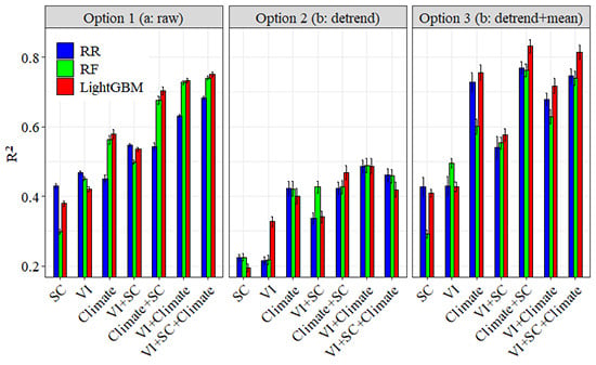
3.2. The Performances of Multi-Models for Predicting Wheat Yield

The results from the first experiment (Figure 4a) distinguish both the shared and unique information of the different predictor variables. A ranking of those combinations from high to low ranges from: “VI + Climate + SC” (R2, 0.68~0.75) > “VI + Climate” (0.63~0.73) > “Climate +SC” (0.54~0.70) > “VI + SC” (0.50~0.55) > “Climate” (0.45~0.58) > “VI” (0.41~0.47) > “SC” (0.30~0.43). As expected, the model performances increase with more input variables. For example, the models with VIs, climate and SC data together perform best for raw crop yields. However, the models with only climate data achieve the highest R2, followed by those with VIs and SC factors.
In addition, we compare the performances of three model groups driven by different input variables to explain the spatio-temporal variability of wheat yield (Figure 4). Please note “Raw” data (Option 1) reflects both spatial and temporal variability, while “Detrend” data (Option 2) only reflect inter-annual variability of the wheat yield, and “Detrend + Mean” (Option 3) reflect spatial and inter-annual variability, respectively. Therefore, comparing results between Option 2 and 3 (Option 3 - Option 2) can reveal the differences in explaining spatial variability (Figure A2). The averaged R2 (0.68~0.75) of “Raw” models is higher than that of “Detrend” (0.41~0.46), suggesting that it should be more difficult to predict inter-annual yield variability compared with the yield variability between counties (Figure 4b). Moreover, the combination of “VIs + Climate” predicted the detrended yields more accurately than others, indicating this combination can capture better inter-annual yield variability than other combinations (“VI + Climate” (~0.49) > “Climate + SC” (0.42–0.47) > “VI + Climate + SC” (R2, 0.42–0.46) > “Climate” (0.40–0.42) > “VI + SC” (0.34–0.42) > “VI” (0.22–0.33) > “SC” (0.20–0.22)). Moreover, the prediction R2 of “Raw” (0.68–0.75) is slightly lower than “Detrend + Mean” (0.76–0.83), suggesting that the multi-year linear trend should matter and that removing the linear trend should increase R2 of the predictive model. The combination of “Climate + SC” can achieve the best prediction results for “Detrend + mean” than others (“Climate + SC” (0.76–0.83) > “VI + Climate + SC” (R2, 0.74–0.81) > “VI + Climate” (0.63–0.72) > “Climate” (0.60–0.75) > “VI + SC” (0.54–0.58) > “VI” (0.43–0.50) > “SC” (0.30–0.43)), suggesting that the “SC + Climate” should better capture the spatial and inter-annual yield variability than other options. Furthermore, the prediction R2 of “Detrend + Mean” (0.76–0.83) is much higher than “Detrend” (0.41–0.46), suggesting that capturing spatial yield variability should be easier than capturing inter-annual yield variability. In order to explain which combination can best capture the spatial yield variability, the results of “Option 3 – Option 2” are calculated (Figure. A2), which show that the “SC + Climate” can better capture it than others (~0.34). Finally, the ML models (RF and LightGBM) overall outperform the traditional linear model (RR), largely because the relationships between yield and the variables are non-linear, and the linear model could not well capture their complex relationships.

3.3. Quantifying Unique and Shared Information from Climate and VIs

The results of the first sub-group of the second experiment were shown in Figure 5 to indicate how sequential information (climate and VIs) during different growing stages (early, peak, and late stages) contribute to crop yield prediction. The models developed by all VIs with a specific climate data show an increased R2 ranging from 0.05 to 0.25, especially for LightGBM models (Figure 6a). Moreover, the RR models perform better than RF and LightGBM models when only using VIs data (the black dashed lines), but do worse when using both VIs and climate data. The different performance might be that RR characterized by a linear model could not fully capture the no-linear relationships between climate variables and yield. Additionally, all the R2 of three models have improved significantly (bars above the dashed line in Figure 5a) after combining a specific climate data with VIs, suggesting the climate inputs across the whole growing seasons could provide unique and added information for better yield estimation.
On the other side, the increased R2 (0.01–0.15) with all of climate variables and a specific VIs (Figure 6b) is smaller than those in Figure 5a, except for the RR models with peak VIs. More interestingly, the largest improvement of R2 (0.07~0.15) is found in the models with the peak VIs, while smaller changes for those with the other two stages, especially for the late VIs. The roles of VIs are different because the peak-value vegetation index reflects most crop growth states suffering from both biotic and abiotic stresses, while crop at “Late” stage enters the senescence stage and vegetation index is not a good indicator of biomass and final yield anymore.
We further summarize in the temporal progresses of the three models’ R2 more detail using different combinations of input variables (Figure 6a–c). The consistent temporal patterns have been indicated by all R2 trajectory curves that R2 would increase with more input data being included until it reaches a saturation at the “Peak” stage (i.e., April). The combinations of inputs perform better than only individual either VIs or climate data. Overall, only climate inputs obviously outperform unique VIs, except for the RR model in the “Later” trajectory. Moreover, both climate and their combinations start with a relatively high performance (R2 > 0.4) for the RF and LightGBM models and R2 increases gradually (0.1~0.3) with the growing season moving on, with the largest increase in June (Figure 6b–c). However, only VIs inputs start with a much lower performance (~0.1) and achieve larger increases in performance as crops become mature (R2 increase in 0.3~0.4) (Figure 6a–c). These results might be associated with our modeling framework. For example, the research is explained at a county scale with each county as an independent sample; and all models predict both spatial and temporal variability in the study. More specifically, climate information during the early season usually captures some spatial patterns of yield. Temperature gradient in space is largely maintained from the early to the late growing season. Therefore, early season temperature will capture some yield patterns in space if the yield is correlated with temperature. Consequently, the relatively high predictive performances of models using climate inputs during the early season would attribute largely to their spatial patterns that can capture some spatial variability of yields. In contrast, the early VIs are consistently low in space and provide less information about the spatial pattern of yields.
In addition, the increased values of the individual dataset over time are also calculated (Figure 6d–f). The distinctly consistent patterns of the declined contributions of climate data as wheat grow from the “Early” to the “Late” stages, while increased ones for VIs. These results suggest that as the growing season progresses, the roles from climate have been replaced gradually by those of VIs. Of course, it is worth noting the obvious difference between the roles of climate data in Figure 6 and those in Figure 5. We could primarily ascribe such a disparity to the different experimental design. Figure 5 shows the increased roles of a specific climate/VIs during different stages combining with all VIs/climate information from the whole growth stages, while Figure 6 indicates the accumulative roles of the individual dataset at different monthly scales.

3.4. The Effects of Spatial Information and Soil Properties on Improving Yield Estimation

Comparing with the roles of dynamic variables (climate and satellite data) for improving yield estimation, those of two types of static variables are shown in Figure 7. The results show that both spatial information and soil properties contribute significantly to wheat yield prediction (an increased R2 by 0.05–0.16), especially for spatial information (Figure 7). The underlying reasons might be that elevation, longitude, latitude, and soil properties can characterize county-specific features over a long time, while dynamic factors (climate, VIs, SC factors) capture dynamic states related to yield during the crop growth season. For example, high-yield areas are usually characterized by fertile soils, lower elevations, and other suitable environmental conditions and vice versa for low-yield areas. All such features can be comprehensively represented by spatial information and soil properties, rather than by VIs, climate, or SC factors.

4. Discussion

4.1. The Best Combinations of Explanatory Variables to Explain Spatial or Temporal Variability of Wheat Yield

In the study, three levels of yield data were separated, namely “raw”, “Detrend”, and “Detrend + Mean” (Figure 4). The models, driven by different combinations of inputs (i.e., climate, VIs, and SC), show disparate performances to track spatial or temporal crop yield variability (Figure 4). For example, the combination of VIs and Climate data can best capture inter-annual yield variability, but SC and climate combination capture spatial yield variability, suggesting that VIs and climate are key factors controlling inter-annual yield variability, and SC and climate for yield variability among counties [1,53,67]. These results might be caused by the fac that the information on VIs and climate variables during a specific period might related to the crop yield for that period, while others such as irrigation and fertilizer application can characterize different features among counties and over a long time. No doubt that the combination of the three datasets can predict yield most accurately for tracking both spatial and temporal yield variability (Figure 4); the reason for this accuracy may be that crop growing status is not only affected by abiotic factors, but also by biotic factors [68,69]. For example, high-yielding can be characterized by fertile soils, water conditions, well-educated farmers, good technologies, well-equipped irrigation facilities, and suitable climate conditions. Thus, combinations of multi-source data may be sufficient to predict yield. Additionally, the results also demonstrate capturing inter-annual yield variability is more difficult and challenging than spatial pattern of crop yield. Our findings are in-line with some previous studies [1,70].
Our results also demonstrate our approaches’ capability of predicting wheat yield with a lead time up to two months before the maturity (Figure 6) in China, which shows the R2 reaches its highest value around May. The best model, i.e., LightGBM, can achieve a yield prediction of 0.79 for the predicted R2 in Oct. The model performance and the lead time of our prediction are consistent with or better than the existing prior work, for instance, Cai et al. (2019) shows their yield model can achieve an R2 ranging from 0.5 to 0.73 with about two months of lead time before the harvest time.

4.2. The Unique and Shared Contributions of Different Data Sources for Predicting Crop Yield

The dynamic variables such as the climate and satellite (especially Visible-NIR based VIs) data have been the domain sources for crop monitoring and yield prediction [34,36,71]. Understanding their shared and unique contributions will better predict and monitor crop yield more scientifically and accurately. First, about 53% and 45% of the raw crop yield variability can be explained by only using climate information and VIs, respectively, and a combination of VIs and climate information can attain a better performance, which is better than previous research (Figure 4) [34]. Second, the increased R2 from a specific VIs combing all climate are much smaller than those from a specific climate combing VIs (Figure 5). The finding further substantiates that climate data supplies more information than VIs for accurately estimating wheat yield, or that the information from VIs includes mixed information of land surfaces, rather than that only related to winter wheat growth [8]. Given that the climate data and satellite data have large overlapping amounts of information, our study reveals their unique individual contribution. Third, regarding the contributions of dynamic variables (VIs and climate data) during different stages (the early, peak, and late stages), peak VIs can provide more information than the other two stages (Figure 5b). It is generally accepted that peak VIs strongly associate with biotic or abiotic factors, which eventually determine final yields [17,72]. However, no such differences have been indicated by climate data, suggesting that unique individual information exists across the whole season (Figure 5a), rather than in a specific stage. The results further suggest that climate variables over the entire growing season play vital roles in determining the final wheat yield across China for the past 15 years. Moreover, the contributions for wheat yield of other critical factors such as SC factors, soil properties, and spatial information were identified and isolated for the first time. Those factors can also contribute to explain more yield variability, proving the hypothesis from previous research [1,34]

4.3. Method Comparison

The non-linear ML methods (RF and LightGBM) perform overall better than the traditional linear method (RR) in yield prediction (Figure 4, Figure 5, Figure 6, Figure 7 and Figure 8), and such results have been reported in previous studies [19,63]. This could be explained by the non-linear relationships between variables and crop yields [1,34]. The following findings in the current study would further substantiate this finding: 1) for estimating the raw yields (Figure 4a), the RF and LightGBM models performed much better than the RR model for all combinations including climate data (e.g., climate, climate + SC, climate + VIs, climate + VIs + SC); 2) the RF and LightGBM models have improved more than the RR model when the raw yields are estimated by using climate data rather than by using VIs and SC factors (Figure 5a); 3) the added value of climate data after being combined with all VIs for RR models is smaller than for the RF and LightGBM models, suggesting the linear RR model could not fully capture the non-linear yield responses to climate data. Such responses had been extensively indicated by temperature and precipitation [25,34]. In addition, recent rapid development in artificial intelligence has led to increased development of deep learning (DL) algorithms, which has been successfully applied in various domains and obviously outperform other techniques (e.g., ML). Therefore, DL could then be used for crop yield estimation in further research [65,73].
To validate the model’s generalization, a series of “leave-one-year-out” experiments were conducted by using the best combinations of all variables (e.g., VIs, climate and SC factors), and the results were shown in Figure 8. The highest R2 was found in both 2011 (0.76~0.84) and 2014 (0.78~0.83), while the lowest R2 in 2007 (0.48~0.55), followed by 2002 (0.58~0.66). The worse performances in 2007 and 2002 might have been caused by some extreme events, which significantly lowered yields. Since these models in the study were developed based on a very small number of event records, condition variables capturing the events might not have been sampled during the historical training, and thus the yield predictions in such extreme years will inevitably deviate from the reality. Such findings also highlight that more efforts and a novel method should be focused on yield loss estimation for the extreme yields.

4.4. Some Limitations of this Study

The first limitation is that using the dryland (one of cultivated land) as winter wheat planting area could lead to errors when we extract the area for the input variables (e.g., satellite and climate data), and so for when the aggregated yield is needed [1]. Therefore, detailed winter wheat cover information will best isolate the relevant areas from the input variables. Using the land use data for 2005, 2010, and 2015 to mask cropland cover is feasible to some degree, but the wheat growing area changes yearly [1]. Hence, it is highly essential in future studies to produce more accurate crop classification each year [1,74] to reduce potential errors. Secondly, we only used vegetation indices (VIs) from optical and near infrared. Although these VIs can provide indicators of photosynthetic canopy cover or leaf area index [34,41], other satellite data encompassing diverse spectral ranges contain complementary information on crop growth and yield. Many other options might further improve the crop yield prediction [25,34], such as solar-induced fluorescence (SIF), thermal-based Evapotranspiration (ET), QuikSCAT Ku-band radar backscatter, AMSR-E X-band passive microwave Vegetation Optical Depth (VOD), and so on. For example, the SIF can provide a general proxy of plant photosynthesis [1,34,75]; the thermal bands are correlated with crop growth for closed canopies and water stress [1,38]; passive or active microwave remote sensing data provide canopy biomass; and water content [1]. All those data may provide complementary information than VIs that are used here. Thirdly, our analysis was based on a relatively coarse county level. ML models are more likely to perform better by collecting more field-level data [12], hence more detailed information will be collected at the field-level for further analyses in the future. Finally, due to their complex model structure for both RF and LightGBM models (so-called black box), it is difficult for us to produce testable hypotheses that could potentially provide biological insights into crop growth and final yield. In the future, we need to combine a crop growth model with ML/DL for predicting yield, forecasting, and monitoring disasters at a large spatial scale.

5. Conclusions

In this study, two ML and RR models were applied to predict wheat yield in China based on climate, satellite data, and other data. The results showed that integrating climate data, satellite data and SC factors can achieve the best performance for raw wheat yield prediction. However, the combination of VIs and climate can best capture inter-annual yield variability, and combining SC with climate can capture spatial yield variability. More specifically, the satellite data can gradually capture crop yield variability, but climate information serves as a unique contribution to wheat yield prediction across the entire growing season. By adding spatially locations and soil properties into benchmark results, the performances of all models further improved, suggesting they convey unique information for prediction yield. In addition, a decent yield prediction can be obtained around two months before harvest in the NCP. This study formulates a robust modeling framework to integrate multi-source data and predict crop yield at a large spatial scale. This framework can be applied to other crops and regions.

Author Contributions

Conceptualization, J.C. and Z.Z.; Formal analysis, Z.Z.; Methodology, J.C. and F.T.; Validation, L.Z., Y.L. and J.H.; Writing—original draft, J.C. and Z.Z.; Writing—review & editing, L.Z., Y.L., J.H. and Z.L. All authors have read and agreed to the published version of the manuscript.

Funding

This study was funded by the National Natural Science Foundation of China (41977405, 41621061, 31561143003). F.T was partly supported by the Academy of Finland through projects AI-CropPro (decision no. 316172).

Conflicts of Interest

The authors declare no conflict of interest.

Appendix A

Figure A1. The area of each statistical province from 2001 to 2015.
Remotesensing 12 00750 g0a1
Figure A2. The delta value of prediction R2 (Option 3-Option 2)
Remotesensing 12 00750 g0a2

References

  1. Cai, Y.; Guan, K.; Lobell, D.; Potgieter, A.B.; Wang, S.; Peng, J.; Xu, T.; Asseng, S.; Zhang, Y.; You, L.; et al. Integrating satellite and climate data to predict wheat yield in Australia using machine learning approaches. Agric. Meteorol. 2019, 274, 144–159. [Google Scholar] [CrossRef]
  2. Groten, S.M.E. NDVI—Crop monitoring and early yield assessment of Burkina Faso. Int. J. Remote Sens. 2007, 14, 1495–1515. [Google Scholar] [CrossRef]
  3. He, Z.; Xia, X.; Zhang, Y. Breeding noodle wheat in China. In Asian Noodles: Science, Technology, and Processing; Wiley: Hoboken, NJ, USA, 2010; pp. 1–23. [Google Scholar]
  4. Song, Y.; Linderholm, H.W.; Wang, C.; Tian, J.; Huo, Z.; Gao, P.; Song, Y.; Guo, A. The influence of excess precipitation on winter wheat under climate change in China from 1961 to 2017. Sci. Total Environ. 2019, 690, 189–196. [Google Scholar] [CrossRef] [PubMed]
  5. Zhai, Y.; Shen, X.; Quan, T.; Ma, X.; Zhang, R.; Ji, C.; Zhang, T.; Hong, J. Impact-oriented water footprint assessment of wheat production in China. Sci. Total Environ. 2019, 689, 90–98. [Google Scholar] [CrossRef] [PubMed]
  6. Zhou, H.; Wang, P.; Chen, D.; Shi, G.; Cheng, K.; Bian, R.; Liu, X.; Zhang, X.; Zheng, J.; Crowley, D.E.; et al. Short-term biochar manipulation of microbial nitrogen transformation in wheat rhizosphere of a metal contaminated Inceptisol from North China plain. Sci. Total Environ. 2018, 640, 1287–1296. [Google Scholar] [CrossRef]
  7. Huang, J.; Tian, L.; Liang, S.; Ma, H.; Becker-Reshef, I.; Huang, Y.; Su, W.; Zhang, X.; Zhu, D.; Wu, W. Improving winter wheat yield estimation by assimilation of the leaf area index from Landsat TM and MODIS data into the WOFOST model. Agric. For. Meteorol. 2015, 204, 106–121. [Google Scholar] [CrossRef] [Green Version]
  8. Chen, Y.; Zhang, Z.; Tao, F. Improving regional winter wheat yield estimation through assimilation of phenology and leaf area index from remote sensing data. Eur. J. Agron. 2018, 101, 163–173. [Google Scholar] [CrossRef]
  9. Lobell, D.B.; Hammer, G.L.; McLean, G.; Messina, C.; Roberts, M.J.; Schlenker, W. The critical role of extreme heat for maize production in the United States. Nat. Clim. Chang. 2013, 3, 497–501. [Google Scholar] [CrossRef]
  10. Lesk, C.; Rowhani, P.; Ramankutty, N. Influence of extreme weather disasters on global crop production. Nature 2016, 529, 84–87. [Google Scholar] [CrossRef]
  11. Horie, T.; Yajima, M.; Nakagawa, H. Yield forecasting. Agric. Syst. 1992, 40, 211–236. [Google Scholar] [CrossRef]
  12. Khaki, S.; Wang, L. Crop Yield Prediction Using Deep Neural Networks. Front. Plant Sci. 2019, 10, 621. [Google Scholar] [CrossRef] [Green Version]
  13. Asseng, S.; Cammarano, D.; Basso, B.; Chung, U.; Alderman, P.D.; Sonder, K.; Reynolds, M.; Lobell, D.B. Hot spots of wheat yield decline with rising temperatures. Glob. Chang. Biol. 2017, 23, 2464–2472. [Google Scholar] [CrossRef]
  14. Kogan, F.; Guo, W.; Yang, W.; Harlan, S. Space-based vegetation health for wheat yield modeling and prediction in Australia. J. Appl. Remote Sens. 2018, 12, 026002. [Google Scholar]
  15. Pantazi, X.E.; Moshou, D.; Alexandridis, T.; Whetton, R.L.; Mouazen, A.M. Wheat yield prediction using machine learning and advanced sensing techniques. Comput. Electron. Agric. 2016, 121, 57–65. [Google Scholar] [CrossRef]
  16. Dhakal, K.; Kakani, V.G.; Linde, E. Climate Change Impact on Wheat Production in the Southern Great Plains of the US Using Downscaled Climate Data. Atmos. Clim. Sci. 2018, 8, 143–162. [Google Scholar] [CrossRef] [Green Version]
  17. Chen, Y.; Zhang, Z.; Tao, F.; Wang, P.; Wei, X. Spatio-temporal patterns of winter wheat yield potential and yield gap during the past three decades in North China. Field Crop. Res. 2017, 206, 11–20. [Google Scholar] [CrossRef]
  18. Lobell, D.B.; Thau, D.; Seifert, C.; Engle, E.; Little, B. A scalable satellite-based crop yield mapper. Remote Sens. Environ. 2015, 164, 324–333. [Google Scholar] [CrossRef]
  19. Cao, J.; Zhang, Z.; Wang, C.; Liu, J.; Zhang, L. Susceptibility assessment of landslides triggered by earthquakes in the Western Sichuan Plateau. Catena 2019, 175, 63–76. [Google Scholar] [CrossRef]
  20. Decencière, E.; Cazuguel, G.; Zhang, X.; Thibault, G.; Klein, J.C.; Meyer, F.; Marcotegui, B.; Quellec, G.; Lamard, M.; Danno, R.; et al. TeleOphta: Machine learning and image processing methods for teleophthalmology. Irbm 2013, 34, 196–203. [Google Scholar] [CrossRef]
  21. Rosten, E.; Drummond, T. Machine learning for high-speed corner detection. In Proceedings of the European Conference on Computer Vision, Graz, Austria, 7–13 May 2006; Springer: Berlin, Heidelberg; Volume 3951, pp. 430–443. [Google Scholar] [CrossRef]
  22. Sidorov, G.; Velasquez, F.; Stamatatos, E.; Gelbukh, A.; Chanona-Hernández, L. Syntactic n-grams as machine learning features for natural language processing. Expert Syst. Appl. 2014, 41, 853–860. [Google Scholar] [CrossRef]
  23. Garosi, Y.; Sheklabadi, M.; Conoscenti, C.; Pourghasemi, H.R.; Van Oost, K. Assessing the performance of GIS- based machine learning models with different accuracy measures for determining susceptibility to gully erosion. Sci. Total Environ. 2019, 664, 1117–1132. [Google Scholar] [CrossRef]
  24. Zhao, G.; Pang, B.; Xu, Z.; Peng, D.; Xu, L. Assessment of urban flood susceptibility using semi-supervised machine learning model. Sci. Total Environ. 2019, 659, 940–949. [Google Scholar] [CrossRef]
  25. Cai, Y.; Guan, K.; Peng, J.; Wang, S.; Seifert, C.; Wardlow, B.; Li, Z. A high-performance and in-season classification system of field-level crop types using time-series Landsat data and a machine learning approach. Remote Sens. Environ. 2018, 210, 35–47. [Google Scholar] [CrossRef]
  26. Kussul, N.; Lavreniuk, M.; Skakun, S.; Shelestov, A. Deep Learning Classification of Land Cover and Crop Types Using Remote Sensing Data. IEEE Geosci. Remote Sens. Lett. 2017, 14, 778–782. [Google Scholar] [CrossRef]
  27. Sharma, S.; Ochsner, T.E.; Twidwell, D.; Carlson, J.; Krueger, E.S.; Engle, D.M.; Fuhlendorf, S.D. Nondestructive estimation of standing crop and fuel moisture content in tallgrass prairie. Rangel. Ecol. Manag. 2018, 71, 356–362. [Google Scholar] [CrossRef]
  28. Johnson, M.D.; Hsieh, W.W.; Cannon, A.J.; Davidson, A.; Bédard, F. Crop yield forecasting on the Canadian Prairies by remotely sensed vegetation indices and machine learning methods. Agric. For. Meteorol. 2016, 218, 74–84. [Google Scholar] [CrossRef]
  29. Kaul, M.; Hill, R.L.; Walthall, C. Artificial neural networks for corn and soybean yield prediction. Agric. Syst. 2005, 85, 1–18. [Google Scholar] [CrossRef]
  30. Everingham, Y.; Sexton, J.; Skocaj, D.; Inman-Bamber, G. Accurate prediction of sugarcane yield using a random forest algorithm. Agron. Sustain. Dev. 2016, 36. [Google Scholar] [CrossRef] [Green Version]
  31. Guan, K.; Berry, J.A.; Zhang, Y.; Joiner, J.; Guanter, L.; Badgley, G.; Lobell, D.B. Improving the monitoring of crop productivity using spaceborne solar-induced fluorescence. Glob. Chang. Biol. 2016, 22, 716–726. [Google Scholar] [CrossRef]
  32. Johnson, D.M. An assessment of pre- and within-season remotely sensed variables for forecasting corn and soybean yields in the United States. Remote Sens. Environ. 2014, 141, 116–128. [Google Scholar] [CrossRef]
  33. Vincenzi, S.; Zucchetta, M.; Franzoi, P.; Pellizzato, M.; Pranovi, F.; De Leo, G.A.; Torricelli, P. Application of a Random Forest algorithm to predict spatial distribution of the potential yield of Ruditapes philippinarum in the Venice lagoon, Italy. Ecol. Model. 2011, 222, 1471–1478. [Google Scholar] [CrossRef]
  34. Guan, K.; Wu, J.; Kimball, J.S.; Anderson, M.C.; Frolking, S.; Li, B.; Hain, C.R.; Lobell, D.B. The shared and unique values of optical, fluorescence, thermal and microwave satellite data for estimating large-scale crop yields. Remote Sens. Environ. 2017, 199, 333–349. [Google Scholar] [CrossRef] [Green Version]
  35. Liu, J.; He, X.; Wang, P.; Huang, J. Early prediction of winter wheat yield with long time series meteorological data and random forest method. Trans. CSAE 2019, 35, 158–166. [Google Scholar] [CrossRef]
  36. Newlands, N.K.; Zamar, D.S.; Kouadio, L.A.; Zhang, Y.; Chipanshi, A.; Potgieter, A.; Toure, S.; Hill, H.S.J. An integrated, probabilistic model for improved seasonal forecasting of agricultural crop yield under environmental uncertainty. Front. Environ. Sci. 2014, 2. [Google Scholar] [CrossRef] [Green Version]
  37. Patrignani, A.; Lollato, R.P.; Ochsner, T.E.; Godsey, C.B.; Edwards, J.T. Yield Gap and Production Gap of Rainfed Winter Wheat in the Southern Great Plains. Agron. J. 2014, 106. [Google Scholar] [CrossRef] [Green Version]
  38. Vereecken, H.; Weihermüller, L.; Jonard, F.; Montzka, C. Characterization of Crop Canopies and Water Stress Related Phenomena using Microwave Remote Sensing Methods: A Review. Vadose Zone J. 2012, 11. [Google Scholar] [CrossRef]
  39. Becker-Reshef, I.; Vermote, E.; Lindeman, M.; Justice, C. A generalized regression-based model for forecasting winter wheat yields in Kansas and Ukraine using MODIS data. Remote Sens. Environ. 2010, 114, 1312–1323. [Google Scholar] [CrossRef]
  40. Burke, M.; Lobell, D.B. Satellite-based assessment of yield variation and its determinants in smallholder African systems. Proc. Natl. Acad. Sci. USA 2017, 114, 2189–2194. [Google Scholar] [CrossRef] [Green Version]
  41. Sellers, P.; Berry, J.; Collatz, G.; Field, C.; Hall, F. Canopy reflectance, photosynthesis, and transpiration. III. A reanalysis using improved leaf models and a new canopy integration scheme. Remote Sens. Environ. 1992, 42, 187–216. [Google Scholar] [CrossRef]
  42. Tucker, C.J. Red and photographic infrared linear combinations for monitoring vegetation. Remote Sens. Environ. 1979, 8, 127–150. [Google Scholar] [CrossRef] [Green Version]
  43. Gitelson, A.A.; Viña, A.; Arkebauer, T.J.; Rundquist, D.C.; Keydan, G.; Leavitt, B. Remote estimation of leaf area index and green leaf biomass in maize canopies. Geophys. Res. Lett. 2003, 30. [Google Scholar] [CrossRef] [Green Version]
  44. Huete, A.; Didan, K.; Miura, T.; Rodriguez, E.P.; Gao, X.; Ferreira, L.G. Overview of the radiometric and biophysical performance of the MODIS vegetation indices. Remote Sens. Environ. 2002, 83, 195–213. [Google Scholar] [CrossRef]
  45. Jain, M.; Srivastava, A.; Balwinder, S.; Joon, R.; McDonald, A.; Royal, K.; Lisaius, M.; Lobell, D. Mapping Smallholder Wheat Yields and Sowing Dates Using Micro-Satellite Data. Remote Sens. 2016, 8, 860. [Google Scholar] [CrossRef] [Green Version]
  46. Lopresti, M.F.; Di Bella, C.M.; Degioanni, A.J. Relationship between MODIS-NDVI data and wheat yield: A case study in Northern Buenos Aires province, Argentina. Inf. Process. Agric. 2015, 2, 73–84. [Google Scholar] [CrossRef] [Green Version]
  47. Ray, D.K.; Ramankutty, N.; Mueller, N.D.; West, P.C.; Foley, J.A. Recent patterns of crop yield growth and stagnation. Nat. Commun. 2012, 3, 1293. [Google Scholar] [CrossRef] [PubMed] [Green Version]
  48. Liu, J.; Wiberg, D.; Zehnder, A.J.B.; Yang, H. Modeling the role of irrigation in winter wheat yield, crop water productivity, and production in China. Irrig. Sci. 2007, 26, 21–33. [Google Scholar] [CrossRef] [Green Version]
  49. Mueller, N.D.; Gerber, J.S.; Johnston, M.; Ray, D.K.; Ramankutty, N.; Foley, J.A. Closing yield gaps through nutrient and water management. Nature 2012, 490, 254–257. [Google Scholar] [CrossRef]
  50. Trueblood, M.A.; Arnade, C. Crop Yield Convergence: How Russia’s Yield Performance Has Compared to Global Yield Leaders. Comp. Econ. Stud. 2001, 43, 59–81. [Google Scholar] [CrossRef]
  51. Yu, H.; Qiang, Z.; Peng, S.; Changqing, S. Impacts of drought intensity and drought duration on winter wheat yield in five provinces of North China plain. Acta Geogr. Sin. 2019, 074, 87–102. [Google Scholar] [CrossRef]
  52. Zhang, T.; Yang, X.; Wang, H.; Li, Y.; Ye, Q. Climatic and technological ceilings for Chinese rice stagnation based on yield gaps and yield trend pattern analysis. Glob. Chang. Biol. 2014, 20, 1289–1298. [Google Scholar] [CrossRef]
  53. Tao, F.; Zhang, Z.; Zhang, S.; Zhu, Z.; Shi, W. Response of crop yields to climate trends since 1980 in China. Clim. Res. 2012, 54, 233–247. [Google Scholar] [CrossRef]
  54. Liu, J.; Kuang, W.; Zhang, Z.; Xu, X.; Qin, Y.; Ning, J.; Zhou, W.; Zhang, S.; Li, R.; Yan, C. Spatiotemporal characteristics, patterns, and causes of land-use changes in China since the late 1980s. J. Geogr. Sci. 2014, 24, 195–210. [Google Scholar] [CrossRef]
  55. Liu, J.; Liu, M.; Tian, H.; Zhuang, D.; Zhang, Z.; Zhang, W.; Tang, X.; Deng, X. Spatial and temporal patterns of China’s cropland during 1990–2000: An analysis based on Landsat TM data. Remote Sens. Environ. 2005, 98, 442–456. [Google Scholar] [CrossRef]
  56. Boken, V.K.; Shaykewich, C.F. Improving an operational wheat yield model using phenological phase-based Normalized Difference Vegetation Index. Int. J. Remote Sens. 2010, 23, 4155–4168. [Google Scholar] [CrossRef]
  57. Abatzoglou, J.T.; Dobrowski, S.Z.; Parks, S.A.; Hegewisch, K.C. TerraClimate, a high-resolution global dataset of monthly climate and climatic water balance from 1958–2015. Sci. Data 2018, 5, 170191. [Google Scholar] [CrossRef] [Green Version]
  58. Shangguan, W.; Dai, Y.; Liu, B.; Ye, A.; Yuan, H. A soil particle-size distribution dataset for regional land and climate modelling in China. Geoderma 2012, 171, 85–91. [Google Scholar] [CrossRef]
  59. Hoerl, A.E.; Kennard, R.W. Ridge Regression: Biased Estimation for Nonorthogonal Problems. Technometrics 1970, 12, 55–67. [Google Scholar] [CrossRef]
  60. Hernandez, J.; Lobos, G.; Matus, I.; del Pozo, A.; Silva, P.; Galleguillos, M. Using Ridge Regression Models to Estimate Grain Yield from Field Spectral Data in Bread Wheat (Triticum aestivum L.) Grown under Three Water Regimes. Remote Sens. 2015, 7, 2109–2126. [Google Scholar] [CrossRef] [Green Version]
  61. Ruppert, D. The Elements of Statistical Learning: Data Mining, Inference, and Prediction. J. Am. Stat. Assoc. 2004, 99, 567. [Google Scholar] [CrossRef]
  62. Breiman, L. Random forests. Mach. Learn. 2001, 45, 5–32. [Google Scholar] [CrossRef] [Green Version]
  63. Youssef, A.M.; Pourghasemi, H.R.; Pourtaghi, Z.S.; Al-Katheeri, M.M. Landslide susceptibility mapping using random forest, boosted regression tree, classification and regression tree, and general linear models and comparison of their performance at Wadi Tayyah Basin, Asir Region, Saudi Arabia. Landslides 2015, 13, 839–856. [Google Scholar] [CrossRef]
  64. Sun, X.; Liu, M.; Sima, Z. A novel cryptocurrency price trend forecasting model based on LightGBM. Financ. Res. Lett. 2018. [Google Scholar] [CrossRef]
  65. Ke, G.; Meng, Q.; Finley, T.; Wang, T.; Chen, W.; Ma, W.; Ye, Q.; Liu, T.-Y. Lightgbm: A highly efficient gradient boosting decision tree. In Proceedings of the Thirty-First Conference on Neural Information Processing System, Long Beach, CA, USA, 4 December 2017. [Google Scholar]
  66. Zhang, W.; Quan, H.; Srinivasan, D. Parallel and reliable probabilistic load forecasting via quantile regression forest and quantile determination. Energy 2018, 160, 810–819. [Google Scholar] [CrossRef]
  67. Wang, P.; Zhang, Z.; Song, X.; Chen, Y.; Wei, X.; Shi, P.; Tao, F. Temperature variations and rice yields in China: Historical contributions and future trends. Clim. Chang. 2014, 124, 777–789. [Google Scholar] [CrossRef]
  68. Hatfield, J.; Gitelson, A.A.; Schepers, J.S.; Walthall, C. Application of spectral remote sensing for agronomic decisions. Agron. J. 2008, 100, S117–S131. [Google Scholar] [CrossRef] [Green Version]
  69. Mahlein, A.-K.; Oerke, E.-C.; Steiner, U.; Dehne, H.-W. Recent advances in sensing plant diseases for precision crop protection. Eur. J. Plant Pathol. 2012, 133, 197–209. [Google Scholar] [CrossRef]
  70. Lobell, D.B. The use of satellite data for crop yield gap analysis. Field Crop. Res. 2013, 143, 56–64. [Google Scholar] [CrossRef] [Green Version]
  71. Manjunath, K.R.; Potdar, M.B.; Purohit, N.L. Large area operational wheat yield model development and validation based on spectral and meteorological data. Int. J. Remote Sens. 2010, 23, 3023–3038. [Google Scholar] [CrossRef]
  72. Zhang, Z.; Wang, P.; Chen, Y.; Song, X.; Wei, X.; Shi, P. Global warming over 1960–2009 did increase heat stress and reduce cold stress in the major rice-planting areas across China. Eur. J. Agron. 2014, 59, 49–56. [Google Scholar] [CrossRef]
  73. You, J.; Li, X.; Low, M.; Lobell, D.; Ermon, S. Deep gaussian process for crop yield prediction based on remote sensing data. In Proceedings of the Thirty-First AAAI Conference on Artificial Intelligence, San Francisco, CA, USA, 4 February 2017. [Google Scholar]
  74. Wardlow, B.D.; Egbert, S.L. Large-area crop mapping using time-series MODIS 250 m NDVI data: An assessment for the U.S. Central Great Plains. Remote Sens. Environ. 2008, 112, 1096–1116. [Google Scholar] [CrossRef]
  75. Guanter, L.; Zhang, Y.; Jung, M.; Joiner, J.; Voigt, M.; Berry, J.A.; Frankenberg, C.; Huete, A.R.; Zarco-Tejada, P.; Lee, J.E.; et al. Global and time-resolved monitoring of crop photosynthesis with chlorophyll fluorescence. Proc. Natl. Acad. Sci. USA 2014, 111, E1327–E1333. [Google Scholar] [CrossRef] [PubMed] [Green Version]
Figure 1. The location of study area. (a) The main winter wheat producing provinces (black line) and counties (orange line), which includes ~76% of the total wheat yield in China; the green shading refers to winter wheat cropping areas. (b) The scope of the China and provincial boundaries (gray line).
Remotesensing 12 00750 g001
Figure 2. A typical example to illustrate the differences in spatial and temporal patterns of data from Options 1–3. Option 1 uses raw county-level data (the red dashed line shows its linear fit) (a); Option 2 removes the linear trend (the red line in Option 1) from the raw data (b), and Option 3 adds the multi-year average of the raw county-level data into the Option 2 data (c); (e)–(g) express the spatial patterns of the three types of yields corresponding to each Option.
Remotesensing 12 00750 g002
Figure 3. Fifteen-year-averaged (2001–2015) spatial patterns after normalization of crop yield (a), the satellite-based variables (bd), climate variables (ei), socio-economic factors (jn) and for all counties in the study region. Note: all of the data have a mean of zero and standard deviation of one; b–i are based on March of every year.
Remotesensing 12 00750 g003
Figure 4. The model performances (predicted R2) of the three methods separated by the three Options with different inputs for the entire growing season. (a) “Raw”; (b) “Detrend”; and (c) “Detrend+Mean”. The blue color is for RR, green for RF and red for LightGBM. The error bars are one standard deviation of predicted R2 from 100 ensembles by randomly dividing training and testing datasets.
Remotesensing 12 00750 g004
Figure 5. (a) The model performance (predicted R2) using VIs during the whole growing season and climate data during a specific stage, either for Early (Oct. and Feb.), or Peak (Mar. and Apr.), or Late stage (Jun. and Jul.). The dashed line in (a) represents the benchmark model performance by only using VIs. (b) The model performance (predicted R2) using the climate data during the whole growing season and VIs during a specific stage (the same stage in (a)). The dashed line in (b) represents the benchmark model performance by only using climate data. The error bars are one standard deviation of predicted R2 from 100 ensembles by randomly dividing training and testing datasets.
Remotesensing 12 00750 g005
Figure 6. The temporal progression of the model performance based on the three methods (RR, RF, and LightGBM). The left panel shows the temporal progress of model performance according to each month (i.e., the prediction at any specific month contains input data covering the period from the beginning of the growing season to that specific month, thus the later period contains more inputs and usually has a higher performance). Blue refers to the model performance of using input sources including climate data and VIs; orange for VIs only inputted; and gray for climate data only. The right panel shows the differences of model performance between combined input sources and VIs only (a blue column indicates the benefits from VIs, calculated by subtracting the orange line from the blue line in the corresponding left panel); and the differences between VI + climate and climate only (a gray column indicates the benefits from VIs, calculated by subtracting the gray line from the blue line in the corresponding panel).
Remotesensing 12 00750 g006
Figure 7. The model performance (predicted R2) after including spatial information and soil properties; the green and red columns mean the R2 after including the soil properties and spatial information in the benchmark model (blue color), respectively. The error bars are one standard deviation of predicted R2 from 100 ensembles obtained by randomly dividing training and testing datasets.
Remotesensing 12 00750 g007
Figure 8. The results of the “leave-one-year-out” experiment across different years. One-year data are selected for testing, while data from other years for training. The worst performance in 2002 and 2007 may be due to extreme events (black for RR, red for RF, and green for LightGBM model).
Remotesensing 12 00750 g008
Table 1. Summary in the collected datasets for winter wheat yield prediction in China. The Tmax, Tmin, Pre, Vpd, and Vap refer to maximum temperatures (°C), minimum temperatures (°C), precipitation (mm), vapor pressure deficit (kPa), and vapor pressure (kPa), respectively; IA, CCF, CAP, TPAM, and ECRA refer to the irrigation area (ha), the consumption of chemical fertilizers (ton), the consumption of agricultural pesticide (CAP), the total power of agricultural machinery (TPAM), and the electricity consumed in rural areas (ECRA), respectively.
CategoryVariablesSpatial ResolutionTemporal ResolutionAvailable RecordsReferences
Crop yield and areaCrop yieldCounty-levelYearly2001-2015http://www.stats.gov.cn
Crop area1 kmFive-year2005, 2010, 2015[45,46]
Satellite dataMOD09A1500 m8-day2001–2018MODIS MOD09A1
DEM90 m20002000SRTM3 V4.1
Climate dataTmin, Tmax, Pre, Vpd, and Vap~4 kmMonthly1958–2018[51]
Socio-economic factorsCAP, CCF, ECRA, IA, and TPAMCounty-levelYearly2001–2015http://www.stats.gov.cn
Soil properties datasoil depth, soil texture, organic carbon content, pH, cation exchange capacity, and bulk density0.00833 (~1 km)20122012[52]
Table 2. EDA results showing the correlations among the 13 variables and correlations between each variable and yields (last column). The input variables were grouped into three categories with different colors: red for climate-related variables, yellow for socio-economic ones, and blue for VIs.
TmaxTminPreVapVpdCAPCCFECRAIATPAMNDVIGCVIEVIYield
Tmax1.000.780.330.580.35−0.09−0.16−0.14−0.19−0.190.480.410.450.03 (**)
Tmin-1.000.670.90−0.22−0.05−0.15−0.14−0.11−0.160.490.430.43−0.08 (***)
Pre--1.000.82−0.58−0.06−0.21−0.16−0.14−0.190.320.280.20−0.40 (***)
Vap---1.00−0.52−0.06−0.19−0.19−0.11−0.200.420.380.33−0.23 (***)
Vpd----1.00−0.010.030.03−0.090.010.010.000.090.29 (***)
CAP-----1.000.420.080.370.420.050.040.050.10 (***)
CCF------1.000.570.830.82−0.12−0.13−0.090.16 (***)
ECRA-------1.000.460.50−0.09−0.09−0.070.12 (***)
IA--------1.000.74−0.16−0.16−0.130.09 (***)
TPAM---------1.00−0.10−0.10−0.070.16(***)
NDVI----------1.000.990.970.31 (***)
GCVI-----------1.000.970.39 (***)
EVI------------1.000.33 (***)
Note: double asterisk ** and threefold asterisks (***) indicate a correlation coefficient (r) with statistical significance levels of p-value 0.01 and p-value b 0.001, respectively.

