Extended Feature Pyramid Network with Adaptive Scale Training Strategy and Anchors for Object Detection in Aerial Images


Abstract
:1. Introduction
- We propose a new framework called Extended Feature Pyramid Network (EFPN) for object detection in aerial images.
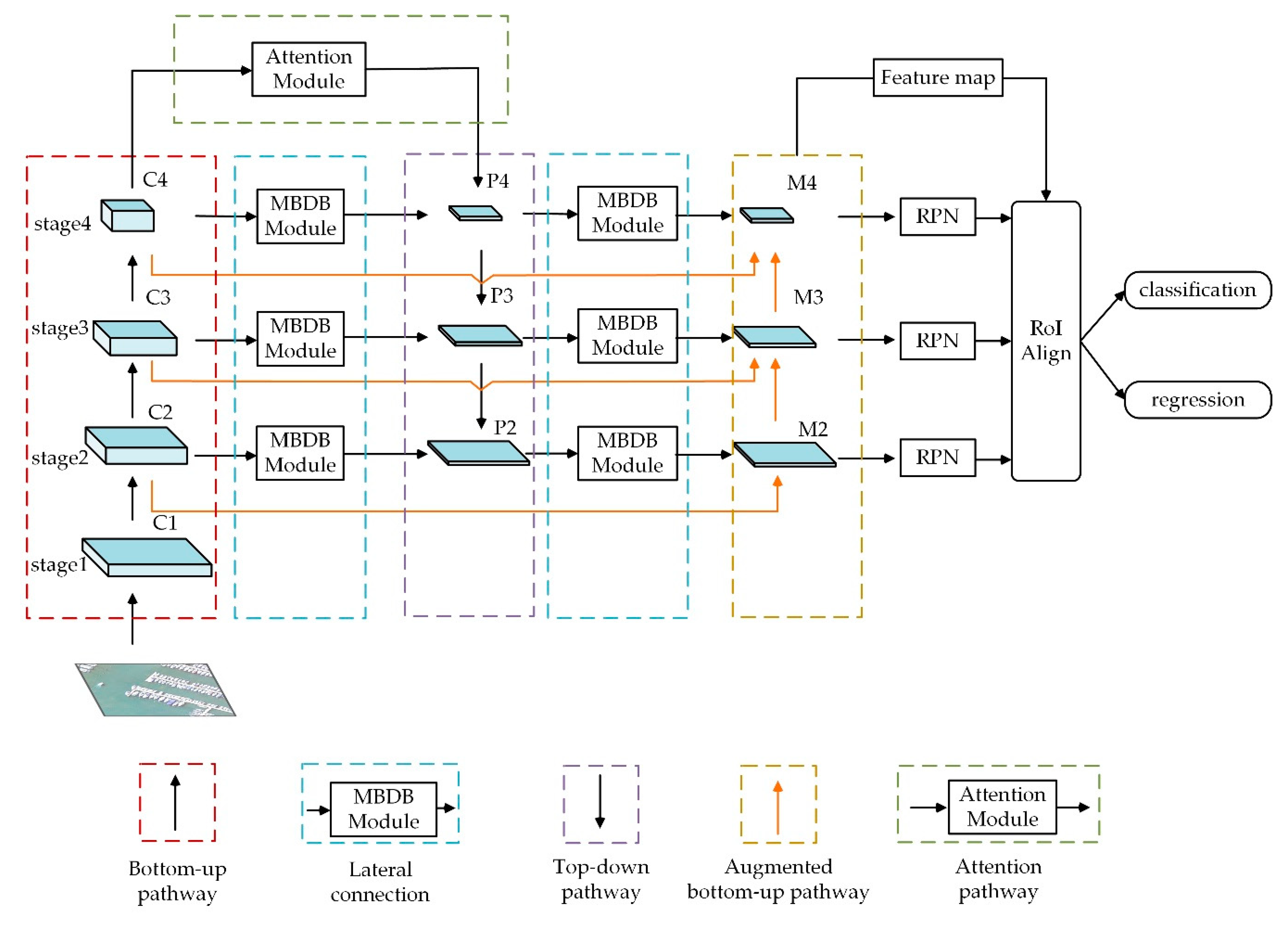
- In the EFPN, we first design the multi-branched dilated bottleneck (MBDB) module in the lateral connections to capture much more semantic information. Then, for better locating the objects, we further design an attention pathway in the deeper layer of EFPN. Finally, an augmented bottom-up pathway is conducted for making shallow layer information easier to spread and further improving performance.
- We propose an adaptive scale training strategy to try to keep the large objects intact after cutting down in the aerial images and improve the recognition ability of the presented network. Meanwhile, we develop a new clustering method for getting adaptive anchors to replace the initial values which are set artificially.
2. Related Works
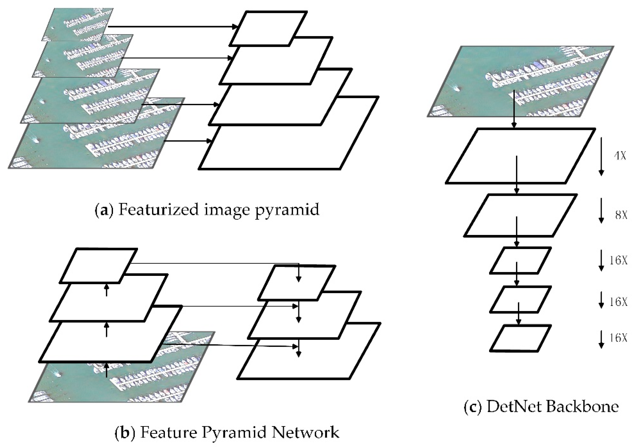
2.1. Multi-Scale Object Detectors
2.2. Dilated Convolution
2.3. K-Means and Mini-Batch k-Means Algorithm
3. Proposed Method
3.1. Extended Feature Pyramid Network
3.1.1. Bottom-Up Pathway
3.1.2. Lateral Connections with MBDB Module
3.1.3. Top-Down Pathway
3.1.4. Attention Pathway
3.1.5. Augmented Bottom-Up Pathway
3.2. Adaptive Scale Training Strategy and Anchors
3.2.1. Adaptive Scale Training Strategy
3.2.2. Adaptive Anchors
4. Dataset and Experimental Settings
4.1. Dataset Description
4.1.1. DOTA-v1.5 Dataset
4.1.2. NWPU VHR-10 Dataset
4.1.3. RSOD Dataset
4.2. Implementation Details
4.3. Evaluation Criteria
5. Results
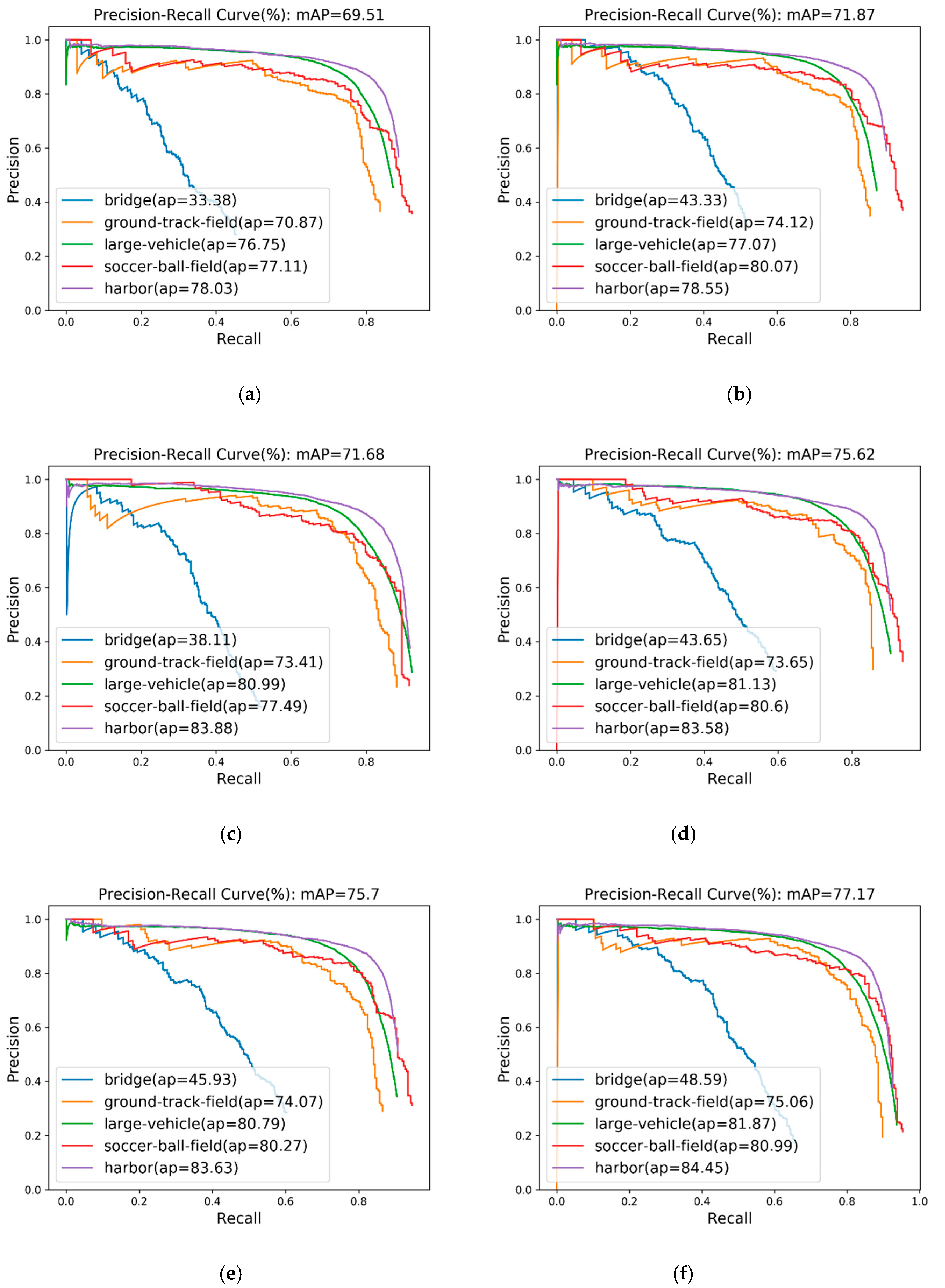
5.1. Ablation Experiments
5.1.1. Ablation for EFPN
5.1.2. Ablation for the Adaptive Scale Training Strategy and Anchors
5.2. Comparison with the-State-of-the-Art Methods
5.2.1. Results on DOTA-v1.5 Dataset
5.2.2. Results on NWPU VHR-10 Dataset
5.2.3. Results on RSOD Dataset
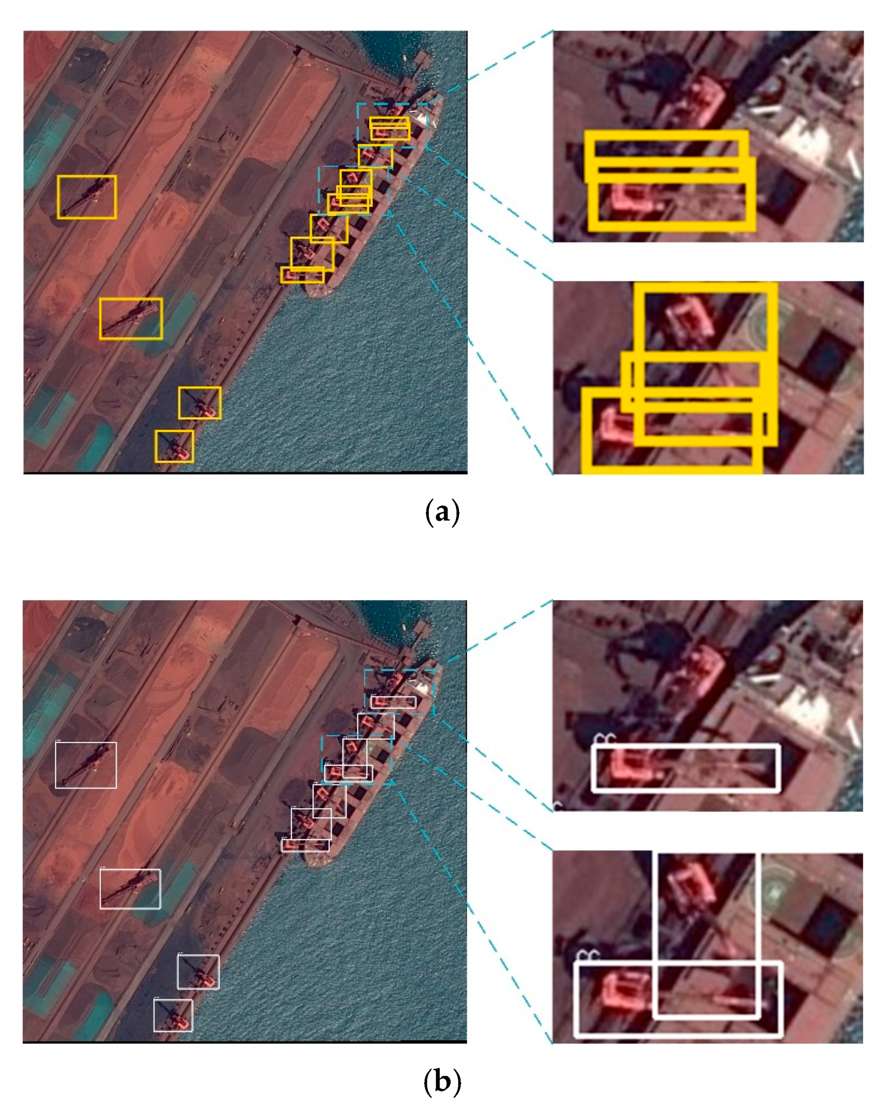
6. Discussion
7. Conclusions
Author Contributions
Funding
Acknowledgments
Conflicts of Interest
References
- Krizhevsky, A.; Sutskever, I.; Hinton, G.E. ImageNet classification with deep convolutional neural networks. In Proceedings of the International Conference on Neural Information Processing Systems (NIPS), Lake Tahoe, NV, USA, 3–8 December 2012; pp. 1097–1105. [Google Scholar]
- Ren, S.; He, K.; Girshick, R.; Sun, J. Faster R-CNN: Towards Real-Time Object Detection with Region Proposal Networks. IEEE Trans. Pattern Anal. Mach. Intell. 2017, 39, 1137–1149. [Google Scholar] [CrossRef] [PubMed] [Green Version]
- Redmon, J.; Farhadi, A. YOLO9000: Better, faster, stronger. In Proceedings of the IEEE Conference on Computer Vision and Pattern Recognition, Honolulu, HI, USA, 22–25 July 2017; pp. 7263–7271. [Google Scholar]
- Chen, C.; Gong, W.; Chen, Y. Object Detection in Remote Sensing Images Based on a Scene-Contextual Feature Pyramid Network. Remote Sens. 2019, 11, 339. [Google Scholar] [CrossRef] [Green Version]
- Qiu, H.; Li, H.; Wu, Q. A2RMNet: Adaptively aspect ratio multi-scale network for object detection in remote sensing images. Remote Sens. 2019, 11, 1594. [Google Scholar] [CrossRef] [Green Version]
- Adelson, E.H.; Anderson, C.H.; Bergen, J.R. Pyramid methods in image processing. RCA Eng. 1984, 29, 33–41. [Google Scholar]
- Dalal, N.; Triggs, B. Histograms of oriented gradients for human detection. In Proceedings of the 2005 IEEE Computer Society Conference on Computer Vision and Pattern Recognition, San Diego, CA, USA, 20–26 June 2005. [Google Scholar]
- Lowe, D.G. Distinctive image features from scale-invariant keypoints. Int. J. Comput. Vis. 2004, 60, 91–110. [Google Scholar] [CrossRef]
- Huang, J.; Rathod, V.; Sun, C. Speed/accuracy trade-offs for modern convolutional object detectors. In Proceedings of the IEEE Conference on Computer Vision and Pattern Recognition, Honolulu, HI, USA, 22–25 July 2017; pp. 7310–7311. [Google Scholar]
- Liu, S.; Qi, L.; Qin, H. Path aggregation network for instance segmentation. In Proceedings of the IEEE Conference on Computer Vision and Pattern Recognition, Salt Lake City, UT, USA, 18–22 June 2018; pp. 8759–8768. [Google Scholar]
- Lin, T.Y.; Dollár, P.; Girshick, R.; He, K.; Hariharan, B.; Belongie, S. Feature pyramid networks for object detection. arXiv 2017, arXiv:1612.03144. [Google Scholar]
- Li, Z.; Peng, C.; Yu, G. Detnet: A backbone network for object detection. arXiv 2018, arXiv:1804.06215. [Google Scholar]
- Yu, F.; Koltun, V.; Funkhouser, T. Dilated residual networks. In Proceedings of the IEEE Conference on Computer Vision and Pattern Recognition, Honolulu, HI, USA, 22–25 July 2017; pp. 472–480. [Google Scholar]
- Chen, L.-C.; Papandreou, G.; Kokkinos, I.; Murphy, K.; Yuille, A.L. Deeplab: Semantic image segmentation with deep convolutional nets, atrous convolution, and fully connected crfs. IEEE Trans. Pattern Anal. Mach. Intell. 2018, 40, 834–848. [Google Scholar] [CrossRef]
- Vaswani, A.; Shazeer, N.; Parmar, N. Attention is all you need. In Proceedings of the Advances in Neural Information Processing Systems 30: Annual Conference on Neural Information Processing Systems, Long Beach, CA, USA, 4–9 December 2017; pp. 5998–6008. [Google Scholar]
- Yan, J.; Wang, H.; Yan, M. IoU-adaptive deformable R-CNN: Make full use of IoU for multi-class object detection in remote sensing imagery. Remote Sens. 2019, 11, 286. [Google Scholar] [CrossRef] [Green Version]
- Uijlings, J.R.R.; Sande, K.; Gevers, T.; Smeulders, A.W.M. Selective Search for Object Recognition. Int. J. Comput. Vis. 2013, 104, 154–171. [Google Scholar] [CrossRef] [Green Version]
- Girshick, R.; Donahue, J.; Darrell, T.; Malik, J. Region-Based Convolutional Networks for Accurate Object Detection and Segmentation. IEEE Trans. Pattern Anal. Mach. Intell. 2015, 38, 142–158. [Google Scholar] [CrossRef] [PubMed]
- Xia, G.S.; Bai, X.; Ding, J. DOTA: A Large-scale Dataset for Object Detection in Aerial Images. arXiv 2017, arXiv:1711.10398. [Google Scholar]
- Cheng, G.; Zhou, P.; Han, J. Learning Rotation-Invariant Convolutional Neural Networks for Object Detection in VHR Optical Remote Sensing Images. IEEE Geosci. Remote Sens. 2016, 54, 7405–7415. [Google Scholar] [CrossRef]
- Long, Y.; Gong, Y.; Xiao, Z.; Liu, Q. Accurate Object Localization in Remote Sensing Images Based on Convolutional Neural Networks. IEEE Geosci. Remote Sens. 2017, 55, 2486–2498. [Google Scholar] [CrossRef]
- Liu, W.; Anguelov, D.; Erhan, D.; Szegedy, C.; Fu, C.; Berg, A.C. SSD: Single Shot Multibox Detector. In Proceedings of the European Conference on Computer Vision, Amsterdam, The Netherlands, 8–16 October 2016; pp. 21–37. [Google Scholar]
- Lin, T.Y.; Goyal, P.; Girshick, R. Focal loss for dense object detection. In Proceedings of the IEEE International Conference on Computer Vision, Venice, Italy, 22–29 October 2017; pp. 2980–2988. [Google Scholar]
- Zhang, S.; Wen, L.; Bian, X. Single-shot refinement neural network for object detection. In Proceedings of the IEEE Conference on Computer Vision and Pattern Recognition, Salt Lake City, UT, USA, 18–22 June 2018; pp. 4203–4212. [Google Scholar]
- Girshick, R. Fast R-CNN. In Proceedings of the IEEE International Conference on Computer Vision, Santiago, Chile, 11–18 December 2015; pp. 1440–1448. [Google Scholar]
- Dai, J.F.; Li, Y.; He, K.M.; Sun, J. R-FCN: Object Detection via Region-based Fully Convolutional Networks. arXiv 2016, arXiv:1606.06409. [Google Scholar]
- Cai, Z.; Fan, Q.; Feris, R.S. A unified multi-scale deep convolutional neural network for fast object detection. In Proceedings of the European Conference on Computer Vision, Amsterdam, The Netherlands, 8–16 October 2016; pp. 354–370. [Google Scholar]
- Zhang, Y.; Gong, W.; Sun, J. Web-Net: A Novel Nest Networks with Ultra-Hierarchical Sampling for Building Extraction from Aerial Imageries. Remote Sens. 2019, 11, 1897. [Google Scholar] [CrossRef] [Green Version]
- Feizollah, A.; Anuar, N.B.; Salleh, R. Comparative study of k-means and mini batch k-means clustering algorithms in android malware detection using network traffic analysis. In Proceedings of the 2014 International Symposium on Biometrics and Security Technologies (ISBAST), Kuala Lumpur, Malaysia, 26–27 August 2014; IEEE: Piscataway, NJ, USA, 2014; pp. 193–197. [Google Scholar]
- He, K.; Gkioxari, G.; Dollar, P. Mask R-CNN. IEEE Trans. Pattern Anal. Mach. Intell. 2017, 99, 1. [Google Scholar] [CrossRef]
- Xie, S.; Girshick, R.; Dollar, P.; Tu, Z.; He, K. Aggregated Residual Transformations for Deep Neural Networks. arXiv 2017, arXiv:1611.05431. [Google Scholar]
- Wang, F.; Jiang, M.; Qian, C. Residual attention network for image classification. In Proceedings of the IEEE Conference on Computer Vision and Pattern Recognition, Honolulu, HI, USA, 22–25 July 2017; pp. 3156–3164. [Google Scholar]
- Woo, S.; Park, J.; Lee, J.Y. Cbam: Convolutional block attention module. In Proceedings of the European Conference on Computer Vision (ECCV), Munich, Germany, 8–14 September 2018; pp. 3–19. [Google Scholar]
- Nair, V.; Hinton, G.E. Rectified linear units improve restricted boltzmann machines. In Proceedings of the 27th International Conference on Machine Learning, Haifa, Israel, 21–24 June 2010; pp. 807–814. [Google Scholar]
- Syakur, M.; Khotimah, B.; Rochman, E.; Satoto, B. Integration k-means clustering method and elbow method for identification of the best customer profile cluster. IOP Conf. Ser. Mater. Sci. Eng. 2018, 336, 012017. [Google Scholar] [CrossRef] [Green Version]
- Girshick, R.; Radosavovic, I.; Gkioxari, G.; Dollar, P.; He, K. Detectron. Available online: https://github.com/facebookresearch/detectron (accessed on 22 January 2018).
- Lin, T.Y.; Maire, M.; Belongie, S. Microsoft coco: Common objects in context. In Proceedings of the European Conference on Computer Vision, Zürich, Switzerland, 6–12 September 2014; pp. 740–755. [Google Scholar]
- Wu, Y.X.; He, K.M. Group Normalization. arXiv 2018, arXiv:1803.08494. [Google Scholar]
- Dai, J.; Qi, H.; Xiong, Y. Deformable convolutional networks. In Proceedings of the IEEE International Conference on Computer Vision, Venice, Italy, 22–29 October 2017; pp. 764–773. [Google Scholar]
- Tayara, H.; Chong, K.T. Object detection in very high-resolution aerial images using one-stage densely connected feature pyramid network. Sensors 2018, 18, 3341. [Google Scholar] [CrossRef] [PubMed] [Green Version]


| Object Classes | Number of Images | Number of Instances | ||
|---|---|---|---|---|
| DOTA-v1.5 | DOTA-v1.0 | DOTA-v1.5 | DOTA-v1.0 | |
| Plane | 198 | 197 | 8072 | 8055 |
| Baseball-diamond | to 121 | 122 | 412 | 415 |
| Bridge | 213 | 210 | 2075 | 2047 |
| Ground-track-field | 180 | 177 | 331 | 325 |
| Small-vehicle | 904 | 486 | 126,686 | 26,126 |
| Large-vehicle | 545 | 380 | 22,400 | 16,969 |
| Ship | 435 | 326 | 32,973 | 28,068 |
| Tennis-court | 308 | 302 | 24,38 | 2367 |
| Basketball-court | 116 | 111 | 529 | 515 |
| Storage-tank | 202 | 161 | 5346 | 5029 |
| Soccer-ball-field | 130 | 136 | 338 | 326 |
| Roundabout | 182 | 170 | 437 | 399 |
| Harbor | 340 | 339 | 6016 | 5983 |
| Swimming-pool | 226 | 144 | 2181 | 1736 |
| Helicopter | 32 | 30 | 635 | 630 |
| Container-crane | 7 | - | 142 | - |
| Method | FPN | MBDB | AP | ABUP | APS | APM | APL | mAP(%) |
|---|---|---|---|---|---|---|---|---|
| FPN [11] | √ | - | - | - | 52.91 | 62.38 | 38.41 | 69.51 |
| FPN+MBDB | √ | √ | - | - | 64.72 | 65.21 | 46.31 | 71.97 |
| FPN+AP | √ | - | √ | - | 60.93 | 64.62 | 48.97 | 72.38 |
| FPN+ABUP | √ | - | - | √ | 63.32 | 63.78 | 42.89 | 71.69 |
| EFPN | √ | √ | √ | √ | 66.11 | 70.16 | 50.38 | 74.67 |
| Method | Params | FLOPs | Average Run Time (s) |
|---|---|---|---|
| FPN [11] | 0.20 s | ||
| FPN+MBDB | 0.21s | ||
| FPN+AP | 0.20s | ||
| FPN+ABUP | 0.21s | ||
| EFPN | 0.23s |
| Method | AS | AA | APS | APM | APL | mAP(%) |
|---|---|---|---|---|---|---|
| FPN [11] | - | - | 52.91 | 62.38 | 38.41 | 69.51 |
| FPN+AS | √ | - | 65.93 | 64.87 | 49.40 | 71.87 |
| FPN+AA | - | √ | 63.31 | 66.49 | 46.42 | 71.68 |
| EFPN | - | - | 66.11 | 70.16 | 50.38 | 74.67 |
| EFPN+AS | √ | - | 67.29 | 71.17 | 52.33 | 75.62 |
| EFPN+AA | - | √ | 67.79 | 70.89 | 50.83 | 75.70 |
| EFPN++ | √ | √ | 70.15 | 72.82 | 53.86 | 77.17 |
| Method | RetinaNet [23] | Faster RCNN [2] | FPN [11] | Ours |
|---|---|---|---|---|
| PL | 69.45 | 71.31 | 77.49 | 86.75 |
| BD | 75.91 | 75.47 | 79.93 | 84.17 |
| BR | 42.45 | 48.8 | 55.12 | 61.28 |
| GTF | 65.24 | 63.78 | 68.03 | 77.45 |
| SV | 34.36 | 51.52 | 61.17 | 77.66 |
| LV | 64.4 | 66.2 | 69.98 | 78.23 |
| SH | 69.26 | 78.19 | 84.87 | 88.35 |
| TC | 88.1 | 90.51 | 89.94 | 90.85 |
| BC | 68.48 | 68.76 | 75.93 | 83.67 |
| ST | 52.08 | 61.84 | 79.22 | 83.64 |
| SBF | 47.96 | 51.45 | 60.83 | 63.42 |
| RA | 63.84 | 69.63 | 71.24 | 76.70 |
| HA | 70.36 | 74.88 | 75.21 | 80.98 |
| SP | 65.41 | 66.83 | 74.51 | 80.99 |
| HC | 43.86 | 50.91 | 57.97 | 77.58 |
| CC | 25.06 | 28.93 | 30.49 | 47.74 |
| mAP(%) | 59.14 | 63.69 | 69.5 | 77.47 |
| Method | YOLOv2 [3] | SSD [22] | Faster R-CNN [2] | R-FCN [26] | Deformable R-FCN [39] | Ours |
|---|---|---|---|---|---|---|
| Airplane | 90.16 | 92.3 | 94.7 | 95.9 | 95.9 | 90.7 |
| SH | 82.22 | 82.42 | 79.8 | 83.4 | 83.8 | 89.2 |
| ST | 20.72 | 52.42 | 55.5 | 65 | 66.8 | 74.5 |
| BD | 94.39 | 97.62 | 92.2 | 94.6 | 95.3 | 87.5 |
| TC | 44.75 | 60.16 | 57.4 | 69.3 | 73.6 | 89.2 |
| BC | 65.74 | 61.84 | 69.1 | 73.9 | 76.8 | 90.8 |
| GTF | 99.85 | 98.67 | 99.5 | 97.4 | 98.1 | 99.3 |
| HA | 66.45 | 75.68 | 72.9 | 77.5 | 77.9 | 88.2 |
| BR | 66.45 | 72.27 | 62.9 | 47.8 | 57.8 | 77.7 |
| Vehicle | 41.82 | 53.82 | 58 | 71.3 | 72.8 | 86.7 |
| mAP(%) | 67.96 | 74.72 | 74.2 | 77.6 | 79.9 | 87.4 |
| Method | YOLOv2 [3] | SSD [22] | Faster R-CNN [2] | R-FCN [26] | Deformable R-FCN [39] | Tayara et al. [40] | Ours |
|---|---|---|---|---|---|---|---|
| Aircraft | 64.8 | 72.5 | 76.6 | 84.3 | 84.1 | 86.25 | 96.3 |
| Oil tank | 93.77 | 92.83 | 95 | 95.7 | 96.8 | 95.98 | 96.9 |
| Overpass | 90.85 | 91.43 | 68 | 74.9 | 82.4 | 94.67 | 89.1 |
| Playground | 99.98 | 97.71 | 96 | 98 | 97.9 | 99.87 | 98.2 |
| mAP(%) | 87.35 | 88.62 | 83.9 | 88.2 | 90.3 | 94.19 | 95.1 |
© 2020 by the authors. Licensee MDPI, Basel, Switzerland. This article is an open access article distributed under the terms and conditions of the Creative Commons Attribution (CC BY) license (http://creativecommons.org/licenses/by/4.0/).
Share and Cite
Guo, W.; Li, W.; Gong, W.; Cui, J. Extended Feature Pyramid Network with Adaptive Scale Training Strategy and Anchors for Object Detection in Aerial Images. Remote Sens. 2020, 12, 784. https://doi.org/10.3390/rs12050784
Guo W, Li W, Gong W, Cui J. Extended Feature Pyramid Network with Adaptive Scale Training Strategy and Anchors for Object Detection in Aerial Images. Remote Sensing. 2020; 12(5):784. https://doi.org/10.3390/rs12050784
Chicago/Turabian StyleGuo, Wei, Weihong Li, Weiguo Gong, and Jinkai Cui. 2020. "Extended Feature Pyramid Network with Adaptive Scale Training Strategy and Anchors for Object Detection in Aerial Images" Remote Sensing 12, no. 5: 784. https://doi.org/10.3390/rs12050784