Hygroscopicity of Different Types of Aerosol Particles: Case Studies Using Multi-Instrument Data in Megacity Beijing, China

Abstract

Water uptake by aerosol particles alters its light-scattering characteristics significantly. However, the hygroscopicities of different aerosol particles are not the same due to their different chemical and physical properties. Such differences are explored by making use of extensive measurements concerning aerosol optical and microphysical properties made during a field experiment from December 2018 to March 2019 in Beijing. The aerosol hygroscopic growth was captured by the aerosol optical characteristics obtained from micropulse lidar, aerosol chemical composition, and aerosol particle size distribution information from ground monitoring, together with conventional meteorological measurements. Aerosol hygroscopicity behaves rather distinctly for mineral dust coarse-mode aerosol (Case I) and non-dust fine-mode aerosol (Case II) in terms of the hygroscopic enhancement factor, $f_{\beta }(RH,{\lambda }_{532})$, calculated for the same humidity range. The two types of aerosols were identified by applying the polarization lidar photometer networking method (POLIPHON). The hygroscopicity for non-dust aerosol was much higher than that for dust conditions with the $f_{\beta }(RH,{\lambda }_{532})$ being around 1.4 and 3.1, respectively, at the relative humidity of 86% for the two cases identified in this study. To study the effect of dust particles on the hygroscopicity of the overall atmospheric aerosol, the two types of aerosols were identified and separated by applying the polarization lidar photometer networking method in Case I. The hygroscopic enhancement factor of separated non-dust fine-mode particles in Case I had been significantly strengthened, getting closer to that of the total aerosol in Case II. These results were verified by the hygroscopicity parameter, κ (Case I non-dust particles: 0.357 $\pm$ 0.024; Case II total: 0.344 $\pm$ 0.026), based on the chemical components obtained by an aerosol chemical speciation instrument, both of which showed strong hygroscopicity. It was found that non-dust fine-mode aerosol contributes more during hygroscopic growth and that non-hygroscopic mineral dust aerosol may reduce the total hygroscopicity per unit volume in Beijing.

1. Introduction

The presence of aerosols has an important impact on the Earth’s climate and environmental changes. It not only indirectly changes the optical and microphysical properties of clouds, but also affects global climate change by changing the radiation balance of the Earth by absorbing and scattering the total incident radiation [1]. However, aerosol loading and properties have high temporal and spatial variations, thus their interactions with the Earth’s climate remain highly uncertain [2,3]. Understanding the mechanism of changes in aerosol characteristics in the atmosphere is of great significance for studying their effects on the Earth’s climate and its changes. A key factor influencing aerosol properties is water vapor, which may be uptaken by aerosol particles [4,5] to alter their optical and microphysical properties, especially scattering and absorption [6].

The sensitivity of aerosol particles to water vapor is usually measured by the hygroscopic enhancement factor that is a function of the aerosol light scattering coefficient with respect to changes in relative humidity (RH) and wavelength (λ) [f_β(RH, λ)]. Kuang (2016) first observed the deliquescence of aerosols in the North China Plain using the humidified nephelometers [7]. Aerosol hygroscopicity is also described by hygroscopic growth factor (GF), which is defined as the ratio of the wet particle diameter at a high RH to that of the dry particle [8] ( Meier et al., 2009). Wang (2017) used hygroscopic and volatile tandem differential mobility analyzer (H/V-TDMA) to study the moisture absorption and volatility characteristics of submeter aerosols under controlled conditions [9]. In addition, the hygroscopicity parameter (κ) is used to describe water uptake ability of different types of aerosols; the κ of mixed aerosol can be obtained from the volume fractions of different chemical components in the aerosol following the method of the Zdanovskii–Stokes–Robinson (ZSR) mixing rule [10,11,12]. Some researchers also use f_β(RH, λ) and GF to derive κ [13,14].

Most of these studies focused on the hygroscopicity of fine-mode spherical aerosol particles. Coarse-mode aerosols of irregular shapes such as dust and sea salt aerosols are also subject to hygroscopic growth in a more complex manner [15,16]. A water-absorbing process has been observed to occur on the surface layer of mineral dust particles, changing their apparent morphological properties, thus impacting dust–cloud interactions [17]. Laboratory studies help gain a deep insight into heterogeneous chemistry processes taking place on dust particles as a result of water-induced swelling and the ensuing changes in their optical properties [18]. While there have existed many studies on aerosol hygroscopicity using in situ and laboratory observation data, there have been relatively few studies in open atmospheric environment conditions in China whose aerosols are heavy and complex with significant impact on regional climate and environment [3,19]. With the increasing amount of lidar measurements, attempts have been made to derive the hygroscopicity of atmospheric aerosols under certain atmospheric conditions [20,21,22,23,24].

In this study, we attempt to investigate differences in the hygroscopic growth between two common types of aerosols observed in Beijing, dust aerosol and non-dust aerosol, using lidar data acquired during a field experiment from December 2018 to March 2019 by choosing two somewhat representative cases. One case corresponds to background fine-mode aerosol, and the other, aerosol mixed with dust particles. Section 2 describes the instruments and methodology. Section 3 shows and discusses the results of the study. The last section is a summary of the whole study.

2. Instruments and Methodology

2.1. Experiment Site

The observation site (Nan Jiao, NJ) is situated near the fifth-ring beltway in southern Beijing (39.81° N, 116.5° E), which is a basic climate observation site of the China Meteorological Administration (Figure 1). It hosts the most comprehensive meteorological observation instruments. The high population density and rapid economic development of the Beijing megacity have led to serious emissions of pollution in the area. A series of observational experiments was carried out here starting in August 2017 with the deployment of a large suite of instruments measuring virtually all aspects of aerosol properties (physical, chemical, optical, and hygroscopic) as summarized in Li (2019) [25]. From December 2018 to March 2019, haze and dust aerosols were dominant at the site. Enhanced observations were thus conducted then to study the mixed state and morphological changes of different chemical components leading to different characteristics of atmospheric pollutant aerosol.

2.2. Instruments

2.2.1. Lidar Systems

This study used two kinds of lidar systems. One system was the micropulse lidar system. It can acquire aerosol vertical optical profiles. It works through a low-energy (6–8 $\mathsf{\mu }\mathrm{J}$) Nd: YVO4 laser with high frequency (2500 Hz) at 532 nm [26]. It can provide continuous profile data with 30 s temporal resolution and 30 m vertical resolution. This system can make polarization measurements at the 532 nm channel. Based on the parallel and vertical corrected signals collected by the Micro Pulse Lidar (MPL), the linear volume depolarization ratio was obtained characterizing the shape of aerosol particles per unit volume. The other system used simultaneously was the Raman lidar system that has three channels of 355 nm, 532 nm, and 1064 nm. It works through a high-energy (~1.2 $\mathrm{J}$) Nd: YAG laser with a 20 Hz frequency. The 7.5 vertical resolution and 15 min temporal resolution profile data can be obtained by our Raman system. Each observation used in this study was the mean of 5000 laser pulses emitted at a frequency of 20 Hz during the interval of 5 min [22]. The Raman lidar system receives 532 nm and 1064 nm atmospheric Mie-scattering signals and vibration–rotation Raman-scattering (355 nm, 386 nm, and 407 nm) signals. These signals are processed to infer water vapor, clouds, and aerosols. This study used extinction ($\sigma$), backscattering coefficient ($\beta$), volume depolarization ratio profiles at 532 nm from this MPL and water vapor profiles (retrieved at 386 nm and 407 nm vibrating Raman channels) from the Raman lidar. The temporal and spatial resolutions of the data from both lidar systems were unified to 15 min and 30 m, respectively, to ensure data consistency.

2.2.2. Aerosol Chemical Speciation Monitor

The aerosol chemical speciation monitor (ACSM) equipped with a fine particulate matter (PM_2.5) inlet impactor was used to detect the chemical characteristics of the aerosols and obtain the mass concentrations of chemical components including sulfate, nitrate, ammonium, chloride, and organics in real time [27,28]. It collects samples at 15 min intervals. First, submicron aerosol particles enter into the aerodynamic particle-focusing lens. After that, the aerosol comes into the particle composition analysis chamber and the particle beam impacts a flash vaporizor with a temperature of about 600 °C and is then ionized through a 70 eV electron impact [29]. Ng (2011) and Sun (2018) provide more details about the operation of the ACSM and its applications [29,30].

2.2.3. Particle Sizers

A nano-scanning mobility particle sizer (Nano-SMPS, model 3756, TSI Inc., Shoreview, MN, USA), a scanning mobility particle sizer (SMPS, model 3938, TSI Inc.), and an aerodynamic particle sizer (APS, model 3321, TSI Inc.) monitored the particle size distributions of the aerosols. These instruments measure particle size distributions and number distributions in real time and in size ranges of 0.00198–0.0649 nm (Nano-SMPS), 0.01–600 nm (SMPS), and 500–20,000 nm (APS). The Nano-SMPS and SMPS use electrostatic classifiers to charge particles, classify particles, and count particles using a condensation particle counter [31]. The APS measures particle velocities, which are then related to particle size through a laser scan technique to calculate particle diameters [31]. Through the relationship between the aerodynamic particle size and Stokes’ particle size [32], data from these three instruments were combined to get a full spectrum distribution of particles from ultrafine to coarse throughout the day. Therefore, the particle spectrum distribution of aerosols at any time of day can be obtained.

2.2.4. Radiosondes and PM Measurement Instruments

L-band GTS1 digital radiosondes are launched twice a day at the NJ site (at ~1115 and ~2315 UTC), collecting data with a 1 s temporal resolution [33]. The GTS1 detector, which takes ~40 min to reach 10 km, provides atmospheric RH profiles with resolution of 1.0%, temperature profiles with resolution of 0.1 °C, and pressure profiles with resolution of 0.1 hPa.

The data used in this study were the calibrated and quality-controlled PM_2.5 and PM₁₀ data acquired from the China National Environmental Monitoring Center (CNEMC) [34,35] of the 1480 PM concentration measurement stations across China, from a station about 2 km from NJ. More details of the instruments we use are listed in

Table 1. List of instruments and parameters.

Instruments	Parameters	Type	Time Resolution	Vertical Spatial Resolution
MPL	Extinction coefficient profile, backscatter coefficient profile, volume depolarization ratio profile	SigmaSpace micropulse lidar system 4202	30 s	30 m
Raman Lidar	Water vapor mixing ratio profile	Vibrational–Rotation polarization Raman lidar	15 min	7.5 m
ACSM	Aerosol chemical composition	Aerodyne Q-ACSM	15 min
SMPS	Particle number size distribution (0.01~0.05 μm)	TSI 3938	5 min
APS	Particle number size distribution (0.5~20 μm)	TSI 3321	5 min
Nano-SMPS	Particle number size distribution (5 nm~0.05 μm)	TSI 3756	5 min
Radiosondes	Temperature profile, relative humidity profile, water vapor mixing ratio profile	L-band GTS1, GRAW	Twice a day (11:00 and 23:00 UTC)	one data per second during ascent

.

2.3. Methodology

2.3.1. Retrieval of Aerosol Optical Depth, Water Vapor, and RH Profiles

When the laser beam emitted by a lidar passes vertically through the atmosphere, the energy $P(z)$ of the echo signal at height $z$ is determined through the lidar equation:

$$P(z)=P_{0}C{z}^{-2}\left[{\beta }_{\mathrm{aer}}(z)+{\beta }_{\mathrm{mol}}(z)\right]T_{\mathrm{aer}}^2(z)T_{\mathrm{mol}}^2(z),$$

(1)

where $P_0$ is the total energy of the laser, $C$ is the lidar system constant, ${\beta }_1(z)$ and ${\beta }_2(z)$ are, respectively, the aerosol particles and air molecules backscattering coefficients. $T_1(z)=\exp [-{\int }_0^Z{\alpha }_1(z)dz]$ is the transmittance of the aerosol, $T_2(z)=\exp [-{\int }_0^Z{\alpha }_2(z)dz]$ is the transmittance of air molecules, and ${\alpha }_1(z)$ and ${\alpha }_2(z)$ are, respectively, the $\sigma$ of aerosol particles and air molecules at height z [36]. The Fernald inversion algorithm [36] retrieved the aerosol $\sigma$ and $\beta$ profiles in this study, which provided an analytic solution to Equation (1) for Mie scattering. Li (2015) provided more details about this algorithm [37].

The water vapor mixing ratio (W) is inverted using the ratio of Raman lidar echo signals of water vapor molecules ($P_{wv}$) to nitrogen molecules ($P_N$) [38]:

$$W(Z)=C_{wv}{∆}_q^w(z_0,z)\frac{P_{wv}(z)}{P_N(z)}$$

(2)

$${∆}_q^w(z_0,z)=\frac{\exp \{-{\int }_{z_0}^z[{\alpha }_{{\lambda }_N}^{aer}(z)+{\alpha }_{{\lambda }_N}^{mol}(z)]dz\}}{\exp \{-{\int }_{z_0}^z[{\alpha }_{{\lambda }_{wv}}^{aer}(z)+{\alpha }_{{\lambda }_{wv}}^{mol}(z)]dz\}}$$

(3)

where $C_{wv}$ is the calibration constant of the Raman lidar, calculated using radiosonde data collected at the same time as the lidar measurements. Two criteria need to be met to ensure the accuracy of the calibration constant calculation within a specified height range: there is no significant change in W, and RH is greater than 30% [39]. The term ${∆}_q^w$ is the correction function for atmospheric transmittance. The parameters ${\alpha }_{{\lambda }_N}^{aer}(z)$ and ${\alpha }_{{\lambda }_{wv}}^{aer}(z)$ are the aerosol extinction coefficients of nitrogen channel and water vapor channel, respectively.

The RH profiles directly measured by radiosondes are converted to W profiles as follows:

$$RH=\frac{p·W}{(3798.554+6.107W)\times {10}^{\frac{7.5t}{237.3+t}}}$$

(4)

where $p$ and $t$ are atmospheric pressure (hPa) and temperature (°C), respectively.

2.3.2. The selection of Hygroscopic Growth Cases

The first step in selecting a hygroscopic growth case is to ensure that the increase in moisture in the aerosol is accompanied by increases in aerosol optical parameters (e.g., $\beta$) and microphysical parameters (e.g., aerosol particle size). Therefore, when studying hygroscopic growth, the aerosol $\beta$ and RH must increase together in the same aerosol layer. The aerosol layer must also be uniformly mixed, otherwise the change in aerosol $\beta$ may not be solely caused by a change in RH. In general, the radiosonde-determined potential temperature ($\theta$) and $W$ of the aerosol layer in question determine the atmospheric mixing conditions of that aerosol layer. The atmosphere is considered uniformly mixed in this study when the variation of $\theta$ is less than 2 °C and the variation of $W$ is less than 2 g/kg [22,40,41,42].

The hygroscopic property of the aerosol is described by $f_{\beta }(RH,\lambda )$, defined as follows:

$$f_{\beta }(RH,\lambda )=\frac{\beta (RH,\lambda )}{\beta (R{H}_{ref},\lambda )}$$

(5)

where $\beta (RH,\lambda )$ and $\beta (R{H}_{\mathrm{ref}},\lambda )$ are the backscattering coefficients of each RH measurement and the reference RH, respectively. The range of RH selected in this study is 65–90%. Equation (5) is usually parameterized using the $\mathrm{H}\mathrm{ä}\mathrm{nel}$ [43] and $\mathrm{Kasten}$ [44] models:

$$H\ddot{a}nel: f_{\beta }(RH,\lambda )={\left[(1-RH)/(1-R{H}_{ref})\right]}^{-\gamma },$$

(6)

$$Kasten: f_{\beta }(RH,\lambda )=a{\left[1-(RH/100)\right]}^{-b}$$

(7)

where γ, a, and b are empirical parameters with γ and b indicating the hygroscopic strength. Both models were used in this study and selected was the parameterization with the best fit according to the least-squares method.

2.3.3. Aerosol Chemical Ion-Pairing Scheme

The hygroscopicity of aerosols is closely related to the various organic and inorganic salts in the atmosphere. The ACSM can provide the mass concentrations and volume fractions of organic and inorganic salts of non-refractory fine PM in the atmosphere [10]. To study the hygroscopic properties of aerosol particles with different chemical compositions and calculate the neutral salts from all ion molar numbers, the ion-pairing scheme was used in this study [45]. Because of its low concentration, the chlorine ion was not considered. The method is described as follows:

$$\begin{array}{c}{n}_{N{H}_{4}N{O}_3}=n_{N{O}_3^{-}},\\ n_{N{H}_{4}HS{O}_4}=min(2n_{S{O}_4^{2-}}-n_{N{H}_4^{+}}+n_{N{O}_3^{-}},n_{N{H}_4^{+}}-n_{N{O}_3^{-}}),\\ n_{{(N{H}_4)}_{2}S{O}_4}=max(n_{N{H}_4^{+}}-n_{N{O}_3^{-}}-n_{S{O}_4^{2-}},0),\\ n_{H_{2}S{O}_4}=max(0,n_{S{O}_4^{2-}}-n_{N{H}_4^{+}}+n_{N{O}_3^{-}}),\\ n_{HN{O}_3}=0,\end{array}$$

(8)

where $n$ refers to the mole number, the “max” and the “min” in the equations indicate maximum and minimum values, respectively. For multicomponent particles, κ is defined by the ZSR mixing rule [8]:

$$\kappa ={\sum }_i{\epsilon }_i{\kappa }_i,$$

(9)

where ${\epsilon }_i$ is the volume fraction of the ith component, and ${\kappa }_i$ is the hygroscopicity parameter for the ith component [46]. The effects of organic compounds are complex, but according to previous studies, its density and ${\kappa }_i$ are assumed to be 1.4 g·cm⁻³ and 0.1, respectively [47]. The volume fraction of each component can be calculated using the parameters listed in

Table 2. The density (in g cm⁻³) and $\kappa$ of the selected compounds.

Species	$\mathbf{N}{\mathbf{H}}_4\mathbf{N}{\mathbf{O}}_3$	$\mathbf{N}{\mathbf{H}}_4\mathbf{H}\mathbf{S}{\mathbf{O}}_4$	${(\mathbf{N}{\mathbf{H}}_4)}_2\mathbf{S}{\mathbf{O}}_4$	${\mathbf{H}}_2\mathbf{S}{\mathbf{O}}_4$	Organics
${\mathrm{Density}}^{}$	1.725	1.78	1.76	1.83	1.4
${\kappa }^{}$	0.68	0.56	0.52	0.91	0.1

.

2.3.4. POLIPHON Method

The polarization lidar photometer networking (POLIPHON) method can be used to separate the optical properties of dust from atmospheric aerosols via the depolarization ratio [48]. This method has been used successfully to separate dust aerosol from other types of aerosols such as separating dust from smoke aerosol produced by biomass burning [49,50] and separating aerosol particles from volcanic ash [51]. It was used here just to differentiate dust and non-dust optical property profiles. The process to separate dust and non-dust backscatter scattering profiles starts with the volume (${\delta }^V$) and particle ($\delta$) linear depolarization ratios [18]:

$${\delta }^V=\frac{P_{cr}}{P_{cr}+P_{co}},$$

(10)

$$\delta =\frac{R\times {\delta }^V\times ({\delta }_{mol}+1)-{\delta }_{mol}\times ({\delta }^V+1)}{R\times ({\delta }_{mol}+1)-({\delta }^V+1)},$$

(11)

where $P_{cr}$ and $P_{co}$ represent signals measured from the parallel and vertical channels, respectively. The parameter $R$ is the backscattering ratio ($R=\frac{{\beta }_m+{\beta }_p}{{\beta }_m}$), ${\delta }_{\mathrm{mol}}$ is the atmospheric molecules depolarization ratio. The depolarization ratios of dust and non-dust are assumed to be relatively stable with height changes; the $\beta$ profiles with dust contributions and with non-dust contributions, ${\beta }_d$ and ${\beta }_{nd}$, respectively, can be calculated [46]:

$${\beta }_d=\beta \frac{(\delta -{\delta }_{nd})(1+{\delta }_d)}{({\delta }_d-{\delta }_{nd})(1+\delta )},$$

(12)

$${\beta }_{nd}=\beta -{\beta }_d,$$

(13)

The dust and non-dust depolarization ratios are ${\delta }_d$ and ${\delta }_{nd}$, respectively, and are assigned values of 0.16 and 0.05, respectively [49]. In this way, coarse-mode dust (non-spherical particles) and fine-mode non-dust particles can be separated and their properties studied separately.

3. Results and Discussion

3.1. Selection of Dust and Non-Dust Cases and Their General Properties

Figure 2 shows the time series of the mass concentrations of PM_2.5 and PM₁₀, the Raman-lidar-measured W, and the 532 nm MPL-measured $\sigma$ and depolarization ratio, measured in NJ, Beijing, from 4–13 February 2019. The shaded areas denote two processes of hygroscopic growth. Case I on around 1115 UTC 5 February 2019 corresponds to the hygroscopic growth with dust particles. Case II on around 1115 UTC 12 February 2019 represents the background aerosol conditions. Using lidar to study the hygroscopic growth of aerosols in the atmosphere must meet certain conditions described in Section 2.3.2 that are distinctly different.

Prior to the time of Case I, there was a transport of dust above 700 m. After the dust transmission process, a local dust event occurred during Case I, which indicated that the depolarization ratio of ~0.2 (Figure 2d) and the mass concentration difference of PM₁₀ and PM_2.5 were large (Figure 2a). The PM₁₀ mass concentration of Case I (~300 μg m⁻³) was greater than that of Case II (<100 μg m⁻³). Figure 3 shows the normalized particle number size distribution (PNSD) in the two cases. It shows there were three obvious particle modes which peaked at the sizes of 0.0018, 0.12, and 1 $\mathsf{\mu }\mathrm{m}$ in Case I. In Case II, the normalized PNSD was generally bimodal, dominated by ultrafine particles. In light of the MPL depolarization ratio and PM results, Case I and II were identified as dust and non-dust (background condition) cases, respectively. From Figure 2b, the upper boundaries of the Case I and Case II layers were located near cloud bases, making the range of RH changes large enough [52]. The locations of the cloud bases can be determined using the 1064 nm range correction signal of the Raman lidar and radiosonde-measured RH values [53]. The weather in Beijing is generally dry, especially in spring and winter. During the entire time series, $W$ in the two hygroscopic growth processes was about 2 g/kg higher than that of other time periods, favourable for hygroscopic growth to occur.

3.2. Case Studies

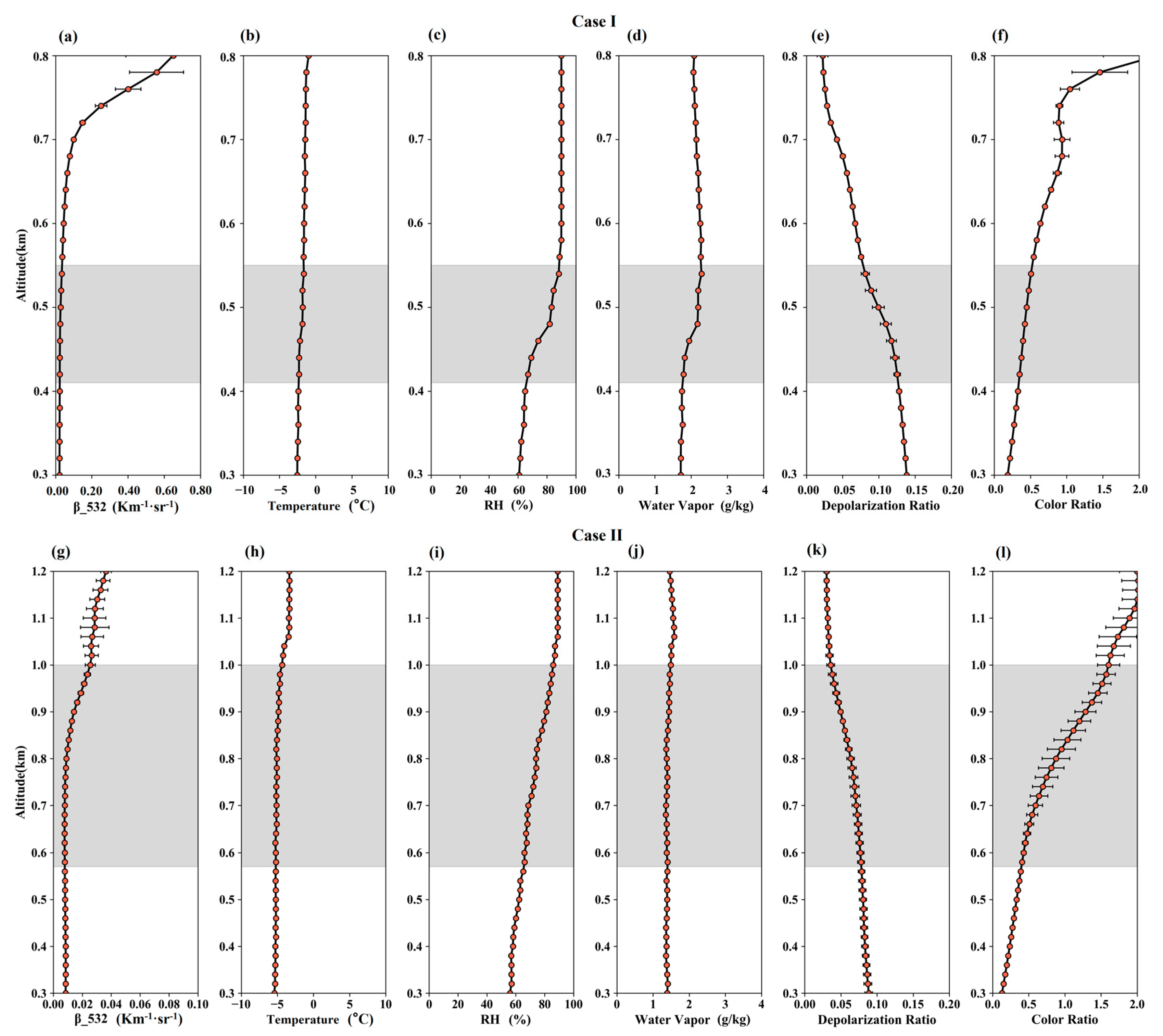
3.2.1. Lidar-Estimated Hygroscopicity

Figure 4 shows the profiles of $W$, RH, $\theta$, β₅₃₂, the depolarization ratio, and the color ratio, which indicates aerosol particle size in each case. In order to ensure that the two cases had the same range of relative humidity, two atmospheric layers were selected to study the hygroscopic growth: 410–540 m for Case I and 580–1000 m for Case II and the relative humidity range of both cases was 65–86%. The $W$ and $\theta$ obtained from radiosondes launched at ~1115 UTC were used to determine the layers of well mixing. As shown in Figure 4 and Table 2, both are generally constant within each layer of each case, indicating uniformly atmospheric mixing and vertical homogeneity in both cases. Therefore, the hygroscopic growth that occurred in both cases, resulting in changes in aerosol optical properties, was most likely caused by the uptake of water [54,55].

When the aerosol layer is uniformly mixed, the variation of aerosol optical properties with height can be considered mainly caused by water uptake in the aerosol layer. Both the β (Figure 4a,g) and RH (Figure 4c,i) increased with altitude within each layer.

Table 3. Range of values and gradient values of the $W$, the $\theta$, the RH, the ${\beta }_{532}$, the depolarization ratio, the color ratio for Case I and Case II.

	Case I			Case II
	Range		Gradient	Range		Gradient
Altitude (m)	410	540	130	580	1000	420
$W$ (${\mathrm{g}\mathrm{kg}}^{-1}$)	1.788	2.285	0.497	1.402	1.488	0.086
$\theta$ (°C)	−2.309	−1.638	0.671	−5.204	−4.352	0.852
${\beta }_{532}$ (${\mathrm{km}}^{-1}{\mathrm{sr}}^{-1}$)	0.023	0.034	0.011	0.008	0.026	0.018
Depolarization ratio	0.125	0.071	−0.054	0.077	0.035	−0.042
Color ratio	0.351	0.544	0.193	0.388	1.60	1.212

shows the specific numerical changes for the two case studies. The volume depolarization ratio, however, decreased with altitude in each layer (Figure 4e,k; Table 3), indicating that the proportion of spherical particles increased with altitude. The volume color ratio (Figure 4f,l; Table 3), which indicates the size of aerosol particles per unit volume, increased in both cases within each layer. Given that the $\beta$ increased with increasing RH in the two layers, hygroscopic growth likely occurred. All these suggest that the aerosol particles gradually grew from the bottom to the top of each layer, accompanied by aerosol particles to become more spherical [18,42,56].

The aerosol particle hygroscopic enhancement factors of the two cases were calculated using the $\mathrm{H}\mathrm{ä}\mathrm{nel}$ and Kasten parameterizations of Equation (4). The initial RH of both cases was 65%.

Table 4. The fitting parameters and coefficients of determination (R²) of the fits using the Kasten and Hänel models.

	Case I			Case II
	a	b	R2	a	b	R2
Kasten	0.68 $\pm$ 0.083	0.33 $\pm$ 0.103	0.93	0.2 $\pm$ 0.017	1.34 $\pm$ 0.091	0.97
	$\mathit{\gamma }$		R2	$\mathit{\gamma }$		R2
Hänel	0.307 $\pm$ 0.100		0.87	1.138 $\pm$ 0.179		0.90

summarizes the fitting results, and Figure 5 shows the $f_{\beta }(RH,\lambda )$ and the fitting results for each case. The Case II hygroscopic growth factor was much stronger than that of Case I. $\beta$ in Case I increased 1.4 times [$f_{\beta -caseI}(86\%)$] in the RH range of 65–86%, while $\beta$ in Case II increased 3.1 times [$f_{\beta -caseII}(86\%)$] in the same RH range, similar to the increase reported in previous studies for other regions [22,23,41,42,54]. Both of the parameters b from the Kasten model and γ from the $\mathrm{H}\mathrm{ä}\mathrm{nel}$ model indicate the strength of hygroscopicity. These parameters in Case I were less than the parameters for Case II (Case I: b = 0.33, $\gamma$ = 0.307; Case II: b = 1.34, $\gamma$ = 1.138) [57]. More intuitively, the color ratio in Case II (Figure 4l) was significantly higher than that in Case I (Figure 4f) within the same range of RH change. Mineral dust particles themselves do not have the characteristics of hygroscopic growth. The hygroscopic growth of dust particles is often due to the change in water absorption of other substances covering the surface of dust particles [58]. Therefore, as stated before, Case I aerosol undergoing hygroscopic growth was aerosol mixed with dust.

3.2.2. Isolating Non-Dust Fine-Mode Aerosol Hygroscopic Properties

To better understand the hygroscopic growth and its dominant influential factors, the one-step POLIPHON method is used to differentiate contributions from dust and non-dust. Figure 6 shows the 532 nm $\beta$ profiles for the mean total, non-dust (mainly fine-mode) and dust (mainly coarse-mode) components. The area of high depolarization ratio in Figure 2d denotes the dust process that was first transmitted to the local area at high altitude and then the local dust process. In Case I, the irregular dust particles with high vertical depolarization ratio mainly concentrated near the ground (below 480 m) and contributed more to the overall $\beta$ in this area. This suggests that dust was generated locally [59,60]. Within the same range of RH, the backscattering coefficient of the non-dust particles increased faster than the total backscattering coefficient.

Figure 7 shows the Case I non-dust particle $f_{\beta }(RH,{\lambda }_{532})$. For a given RH, the $f_{\beta }(RH,{\lambda }_{532})$ of non-dust fine-mode particles in Case I is much higher than that when particles of all modes are considered. The non-dust-particle $f_{\beta }(RH,{\lambda }_{532})$ was fitted using the Kasten parameterization. The Case I non-dust-particle b value is 0.98, which is greater than the Case I total-particle b value (0.33) and closer to the Case II total-particle b value (1.34). The hygroscopic growth intensity of Case I is similar to that of Case II, which represents mainly non-dust fine particles. This suggests that fine-mode non-dust particles play a dominant role in hygroscopic growth. Di Girolamo (2012) observed a similar phenomenon in their study on aged dust particles mixed with maritime, urban, and organic aerosols [61].

3.3. The Influence of Chemical Composition Inferred from ACSM Measurements

Removing dust particles from the mean total profile in the dust case increased the hygroscopic strength of the remaining fine-mode particles, which became closer to that of aerosol in the case of a clean atmosphere. In other words, fine-mode aerosol particles may be instrumental in hygroscopic growth. The specific chemical composition of aerosols in each mode is important when determining $f_{\beta }(RH)$ [62]. Here, the chemical compositions of fine-mode particles in Cases I and II were analyzed. Because the ACSM’s inlet impactor has a diameter of 2. $\mathsf{\mu }\mathrm{m}$, only fine-mode aerosols were considered. Figure 8 shows the percentages of aerosol chemical compositions obtained from the ACSM measurements around the times of the two cases. The chemical compositions in the two cases were similar. Organics dominated in both cases (Case I: 43.2%; Case II: 46.1%). The percentages of sulfate in Cases I and II were 25.1% and 19.3%, and those of nitrate were 19.1% and 21.2%, respectively. The proportions of amine (Case I: 11.3%; Case II: 11.8%) and chloride (~1%) were the smallest. Because of its low percentage and relatively low hygroscopicity, chloride was neglected in this study [10,13,26].

Table 5. Calculated volume fractions (VF) of ${\mathrm{NH}}_4{\mathrm{NO}}_3$, ${\mathrm{NH}}_4{\mathrm{HSO}}_4$, ${({\mathrm{NH}}_4)}_2{\mathrm{SO}}_4$, ${\mathrm{H}}_2{\mathrm{SO}}_4$, and organics, and the hygroscopicity parameter ($\mathit{\kappa }$) for Case I and Case II.

	Case I					Case II
	$\mathbf{N}{\mathbf{H}}_4\mathbf{N}{\mathbf{O}}_3$	$\mathbf{N}{\mathbf{H}}_4\mathbf{H}\mathbf{S}{\mathbf{O}}_4$	${(\mathbf{N}{\mathbf{H}}_4)}_2\mathbf{S}{\mathbf{O}}_4$	${\mathbf{H}}_2\mathbf{S}{\mathbf{O}}_4$	Organics	$\mathbf{N}{\mathbf{H}}_4\mathbf{N}{\mathbf{O}}_3$	$\mathbf{N}{\mathbf{H}}_4\mathbf{H}\mathbf{S}{\mathbf{O}}_4$	${(\mathbf{N}{\mathbf{H}}_4)}_2\mathbf{S}{\mathbf{O}}_4$	${\mathbf{H}}_2\mathbf{S}{\mathbf{O}}_4$	Organics
VF	0.227 $\pm$ 0.019	0.210 $\pm$ 0.093	0.068 $\pm$ 0.090	0	0.493 $\pm$ 0.040	0.252 $\pm$ 0.047	0.089 $\pm$ 0.084	0.136 $\pm$ 0.102	0	0.523 $\pm$ 0.046
$\mathsf{\kappa }$	0.357 $\pm$ 0.024					0.344 $\pm$ 0.026

summarizes the volume fraction and $\mathsf{\kappa }$ values of each case. The $\mathsf{\kappa }$ values were 0.357 and 0.344 for Cases I and II, respectively, suggesting that the fine-mode aerosol hygroscopicity in both cases was relatively strong and approximately the same. This means that the hygroscopicity of aerosols in Beijing depends on fine-mode aerosol particles and that the presence of mineral dust (non-hygroscopic particles) will reduce the overall hygroscopicity to some extent [20,62].

4. Conclusions

An enhanced observation experiment was conducted in the Beijing climate observatory from December 2018 to March 2019. During this time, the hygroscopic growth characteristics of two different atmospheric conditions (dusty, non-dust) were studied using data collected by a ground-based lidar system and radiosondes, and using aerosol particle spectrum and chemical composition information. The increase in the aerosol $\beta$ with increasing RH was used to determine the hygroscopic growth of the aerosols. W and $\theta$ vertical profiles provided additional constraints to the selection of hygroscopic growth cases. During hygroscopic growth, the volume depolarization ratio decreased and the color ratio increased, suggesting that aerosol particles grew larger and became more spherical. However, the hygroscopic enhancement properties of these two different types of aerosols differed. The Kasten and $\mathrm{H}\mathrm{ä}\mathrm{nel}$ parameterization schemes were applied to the two selected cases using a reference RH of 65% in both cases. It was applied to fit the $f_{\beta }(RH,\lambda )$, parameter b at very low values around 0.33 $\pm$ 0.103 for aerosol with mineral dust (Case I), and reaching up to 1.34 $\pm$ 0.091 for aerosol of moderate background loading (Case II). The strength of the hygroscopic growth of the fine-mode clean aerosol case (Case II) was stronger than that of the aerosol mixed with coarse-mode mineral dust (Case I) due to the different types of aerosols in each case. From lidar-measured $\beta$ and depolarization ratios and aerosol particle spectra obtained from particle sizers, the type of aerosol in each case was identified: a mixture of irregularly shaped dust aerosol and non-dust fine-mode aerosol (Case I) and mainly fine-mode clean aerosol (Case II). To study the contribution of each aerosol type in Case I to hygroscopic growth, dust aerosol in Case I was separated from fine-mode aerosol using the POLIPHON method. Within the same range of RH, the non-dust aerosol $\beta$ and the $f_{\beta }(RH,{\lambda }_{532})$ increased much faster than those for the dust component and the overall aerosol. The chemical composition of the background aerosol in two cases obtained by the ACSM was also used to verify the hygroscopic strength of non-dust fine-mode aerosol particles in Case I and in Case II. The hygroscopic strength kappa coefficient of the non-dust fine-mode aerosol in Case I and that for the total aerosol of Case II were similar (Case I: 0.357; Case II: 0.344), representing the general hygroscopic growth of background aerosol in the region. All the results show that fine-mode aerosol particles play a leading role in the process of moisture absorption growth, and the presence of non-hygroscopic dust particles can weaken the total hygroscopicity per unit volume to some extent.

References

1. IPCC. Climate Change 2013: The Physical Science Basis. Contribution of Working Group I to the Fifth Assessment Report of the Intergovernmental Panel on Climate Change; Stocker, T.F., Qin, D., Plattner, G.-K., Tignor, M.M.B., Allen, S.K., Boschung, J., Nauels, A., Xia, Y., Bex, V., Midgley, P.M., Eds.; Cambridge University Press: Cambridge, UK; New York, NY, USA, 2013. [Google Scholar]
2. Kaufman, Y.J.; Tanré, D.; Boucher, O. A satellite view of aerosols in the climate system. Nature 2002, 419, 215–223. [Google Scholar] [CrossRef]
3. Li, Z.; Lau, W.K.-M.; Ramanathan, V.; Wu, G.; Ding, Y.; Manoj, M.G.; Liu, J.; Qian, Y.; Li, J.; Zhou, T.; et al. Aerosol and monsoon climate interactions over Asia. Rev. Geophys. 2016, 54, 866–929. [Google Scholar] [CrossRef]
4. Petters, M.D.; Kreidenweis, S.M. A single parameter representation of hygroscopic growth and cloud condensation nucleus activity. Atmos. Chem. Phys. 2007, 7, 1961–1971. [Google Scholar] [CrossRef] [Green Version]
5. Jin, X.; Wang, Y.; Li, Z.; Zhang, F.; Xu, W.; Sun, Y.; Fan, X.; Chen, G.; Wu, H.; Ren, J.; et al. Significant contribution of organics to aerosol liquid water content in winter in Beijing, China. Atmos. Chem. Phys. Discuss. 2020, 20, 901–914. [Google Scholar] [CrossRef] [Green Version]
6. Zieger, P.; Weingartner, E.; Henzing, J.; Moerman, M.; de Leeuw, G.; Mikkilä, J.; Ehn, M.; Petäjä, T.; Clémer, K.; van Roozendael, M.; et al. Comparison of ambient aerosol extinction coefficients obtained from in-situ, MAX-DOAS and LIDAR measurements at Cabauw. Atmos. Chem. Phys. 2011, 11, 2603–2624. [Google Scholar] [CrossRef] [Green Version]
7. Kuang, Y.; Zhao, C.S.; Ma, N.; Liu, H.J.; Bian, Y.X.; Tao, J.C.; Hu, M. Deliquescent phenomena of ambient aerosols on the North China Plain: Deliquescence of Ambient Aerosols. Geophys. Res. Lett. 2016, 43, 8744–8750. [Google Scholar] [CrossRef]
8. Meier, J.; Wehner, B.; Massling, A.; Birmili, W.; Nowak, A.; Gnauk, T.; Wiedensohler, A. Hygroscopic growth of urban aerosol particles in Beijing (China) during wintertime: a comparison of three experimental methods. Atmos. Chem. Phys. 2009, 16. [Google Scholar]
9. Wang, Y.; Zhang, F.; Li, Z.; Tan, H.; Xu, H.; Ren, J.; Zhao, J.; Du, W.; Sun, Y. Enhanced hydrophobicity and volatility of submicron aerosols under severe emission control conditions in Beijing. Atmos. Chem. Phys. 2017, 17, 5239–5251. [Google Scholar] [CrossRef] [Green Version]
10. Gysel, M.; Crosier, J.; Topping, D.O.; Whitehead, J.D.; Bower, K.N.; Cubison, M.J.; Williams, P.I.; Flynn, M.J.; McFiggans, G.B.; Coe, H. Closure study between chemical composition and hygroscopic growth of aerosol particles during TORCH2. Atmos. Chem. Phys. 2007, 7, 6131–6144. [Google Scholar] [CrossRef] [Green Version]
11. Svenningsson, B.; Rissler, J.; Swietlicki, E.; Mircea, M.; Bilde, M.; Facchini, M.C.; Decesari, S.; Fuzzi, S.; Zhou, J.; Mønster, J.; et al. Hygroscopic growth and critical supersaturations for mixed aerosol particles of inorganic and organic compounds of atmospheric relevance. Atmos. Chem. Phys. 2006, 16. [Google Scholar] [CrossRef] [Green Version]
12. Chang, R.Y.-W.; Slowik, J.G.; Shantz, N.C.; Vlasenko, A.; Liggio, J.; Sjostedt, S.J.; Leaitch, W.R.; Abbatt, J.P.D. The hygroscopicity parameter (κ) of ambient organic aerosol at a field site subject to biogenic and anthropogenic influences: Relationship to degree of aerosol oxidation. Atmos. Chem. Phys. 2010, 10, 5047–5064. [Google Scholar] [CrossRef] [Green Version]
13. Petters, M.D.; Kreidenweis, S.M. A single parameter representation of hygroscopic growth and cloud condensation nucleus activity—Part 3: Including surfactant partitioning. Atmos. Chem. Phys. Discuss. 2012, 12, 22687–22712. [Google Scholar] [CrossRef]
14. Kuang, Y.; Zhao, C.; Tao, J.; Bian, Y.; Ma, N.; Zhao, G. A novel method for deriving the aerosol hygroscopicity parameter based only on measurements from a humidified nephelometer system. Atmos. Chem. Phys. 2017, 17, 6651–6662. [Google Scholar] [CrossRef] [Green Version]
15. Sheridan, P.J.; Delene, D.J.; Ogren, J.A. Four years of continuous surface aerosol measurements from the Department of Energy’s Atmospheric Radiation Measurement Program Southern Great Plains Cloud and Radiation Testbed site. J. Geophys. Res. Atmos. 2001, 106, 20735–20747. [Google Scholar] [CrossRef] [Green Version]
16. Kim, J.; Yoon, S.-C.; Jefferson, A.; Kim, S.-W. Aerosol hygroscopic properties during Asian dust, pollution, and biomass burning episodes at Gosan, Korea in April 2001. Atmos. Environ. 2006, 40, 1550–1560. [Google Scholar] [CrossRef]
17. Tang, M.; Cziczo, D.J.; Grassian, V.H. Interactions of Water with Mineral Dust Aerosol: Water Adsorption, Hygroscopicity, Cloud Condensation, and Ice Nucleation. Chem. Rev. 2016, 116, 4205–4259. [Google Scholar] [CrossRef] [Green Version]
18. Krueger, B.J. The transformation of solid atmospheric particles into liquid droplets through heterogeneous chemistry: Laboratory insights into the processing of calcium containing mineral dust aerosol in the troposphere. Geophys. Res. Lett. 2003, 30, 1148. [Google Scholar] [CrossRef] [Green Version]
19. Li, Z.; Guo, J.; Ding, A.; Liao, H.; Liu, J.; Sun, Y.; Wang, T.; Xue, H.; Zhang, H.; Zhu, B. Aerosol and boundary-layer interactions and impact on air quality. Natl. Sci. Rev. 2017, 4, 810–833. [Google Scholar] [CrossRef]
20. Veselovskii, I.; Goloub, P.; Podvin, T.; Tanre, D.; da Silva, A.; Colarco, P.; Castellanos, P.; Korenskiy, M.; Hu, Q.; Whiteman, D.N.; et al. Characterization of smoke/dust episode over West Africa: comparison of MERRA-2 modeling with multiwavelength Mie-Raman lidar observations. Atmos. Meas. Tech. Discuss. 2018, 11, 949–969. [Google Scholar] [CrossRef] [Green Version]
21. Fernández, A.J.; Apituley, A.; Veselovskii, I.; Suvorina, A.; Henzing, J.; Pujadas, M.; Artíñano, B. Study of aerosol hygroscopic events over the Cabauw experimental site for atmospheric research (CESAR) using the multi-wavelength Raman lidar Caeli. Atmos. Environ. 2015, 120, 484–498. [Google Scholar] [CrossRef]
22. Chen, J.; Li, Z.; Lv, M.; Wang, Y.; Wang, W.; Zhang, Y.; Wang, H.; Yan, X.; Sun, Y.; Cribb, M. Aerosol hygroscopic growth, contributing factors, and impact on haze events in a severely polluted region in northern China. Atmos. Chem. Phys. 2019, 19, 1327–1342. [Google Scholar] [CrossRef] [Green Version]
23. Zhao, G.; Zhao, C.; Kuang, Y.; Tao, J.; Tan, W.; Bian, Y.; Li, J.; Li, C. Impact of aerosol hygroscopic growth on retrieving aerosol extinction coefficient profiles from elastic-backscatter lidar signals. Atmos. Chem. Phys. 2017, 17, 12133–12143. [Google Scholar] [CrossRef] [Green Version]
24. Eichler, H.; Cheng, Y.F.; Birmili, W.; Nowak, A.; Wiedensohler, A.; Brüggemann, E.; Gnauk, T.; Herrmann, H.; Althausen, D.; Ansmann, A. Hygroscopic properties and extinction of aerosol particles at ambient relative humidity in South-Eastern China. Atmos. Environ. 2008, 42, 6321–6334. [Google Scholar] [CrossRef]
25. Li, Z.; Wang, Y.; Guo, J.; Zhao, C.; Cribb, M.C.; Dong, X.; Fan, J.; Gong, D.; Huang, J.; Jiang, M.; et al. East Asian Study of Tropospheric Aerosols and their Impact on Regional Clouds, Precipitation, and Climate (EAST-AIR CPC). J. Geophys. Res. Atmos. 2019. [Google Scholar] [CrossRef] [Green Version]
26. Huang, Z.; Huang, J.; Bi, J.; Wang, G.; Wang, W.; Fu, Q.; Li, Z.; Tsay, S.-C.; Shi, J. Dust aerosol vertical structure measurements using three MPL lidars during 2008 China-U.S. joint dust field experiment. J. Geophys. Res. 2010, 115, D00K15. [Google Scholar] [CrossRef] [Green Version]
27. Zhang, Y.; Du, W.; Wang, Y.; Wang, Q.; Wang, H.; Zheng, H.; Zhang, F.; Shi, H.; Bian, Y.; Han, Y.; et al. Aerosol chemistry and particle growth events at an urban downwind site in North China Plain. Atmos. Chem. Phys. 2018, 18, 14637–14651. [Google Scholar] [CrossRef] [Green Version]
28. Jiang, Q.; Wang, F.; Sun, Y. Analysis of Chemical Composition, Source and Processing Characteristics of Submicron Aerosol during the Summer in Beijing, China. Aerosol Air Qual. Res. 2019, 19, 1450–1462. [Google Scholar] [CrossRef] [Green Version]
29. Ng, N.L.; Herndon, S.C.; Trimborn, A.; Canagaratna, M.R.; Croteau, P.L.; Onasch, T.B.; Sueper, D.; Worsnop, D.R.; Zhang, Q.; Sun, Y.L.; et al. An Aerosol Chemical Speciation Monitor (ACSM) for Routine Monitoring of the Composition and Mass Concentrations of Ambient Aerosol. Aerosol Sci. Technol. 2011, 45, 780–794. [Google Scholar] [CrossRef]
30. Sun, Y.; Xu, W.; Zhang, Q.; Jiang, Q.; Canonaco, F.; Prévôt, A.S.H.; Fu, P.; Li, J.; Jayne, J.; Worsnop, D.R.; et al. Source apportionment of organic aerosol from 2-year highly time-resolved measurements by an aerosol chemical speciation monitor in Beijing, China. Atmos. Chem. Phys. 2018, 18, 8469–8489. [Google Scholar] [CrossRef] [Green Version]
31. Hitchins, J.; Morawska, L.; Wolff, R.; Gilbert, D. Concentrations of submicrometre particles from vehicle emissions near a major road. Atmos. Environ. 2000, 34, 51–59. [Google Scholar] [CrossRef] [Green Version]
32. Covert, D.S.; Wiedensohler, A.; Aalto, P.; Heintzenberg, J.; Mcmurry, P.H.; Leck, C. Aerosol number size distributions from 3 to 500 nm diameter in the arctic marine boundary layer during summer and autumn. Tellus B Chem. Phys. Meteorol. 1996, 48, 197–212. [Google Scholar] [CrossRef] [Green Version]
33. Bian, J.; Chen, H.; Vömel, H.; Duan, Y.; Xuan, Y.; Lü, D. Intercomparison of humidity and temperature sensors: GTS1, Vaisala RS80, and CFH. Adv. Atmos. Sci. 2011, 28, 139–146. [Google Scholar] [CrossRef]
34. Guo, J.-P.; Zhang, X.-Y.; Che, H.-Z.; Gong, S.-L.; An, X.; Cao, C.-X.; Guang, J.; Zhang, H.; Wang, Y.-Q.; Zhang, X.-C.; et al. Correlation between PM concentrations and aerosol optical depth in eastern China. Atmos. Environ. 2009, 43, 5876–5886. [Google Scholar] [CrossRef]
35. Wu, T.; Fan, M.; Tao, J.; Su, L.; Wang, P.; Liu, D.; Li, M.; Han, X.; Chen, L. Aerosol Optical Properties over China from RAMS-CMAQ Model Compared with CALIOP Observations. Atmosphere 2017, 8, 201. [Google Scholar] [CrossRef] [Green Version]
36. Fernald, F.G. Analysis of atmospheric lidar observations: Some comments. Appl. Opt. 1984, 23, 652. [Google Scholar] [CrossRef]
37. Li, C.; Pan, Z.; Mao, F.; Gong, W.; Chen, S.; Min, Q. De-noising and retrieving algorithm of Mie lidar data based on the particle filter and the Fernald method. Opt. Express 2015, 23, 26509. [Google Scholar] [CrossRef]
38. Whiteman, D.N.; Melfi, S.H.; Ferrare, R.A. Raman lidar system for the measurement of water vapor and aerosols in the Earth’s atmosphere. Appl. Opt. 1992, 31, 3068. [Google Scholar] [CrossRef]
39. Miloshevich, L.M.; Vömel, H.; Whiteman, D.N.; Lesht, B.M.; Schmidlin, F.J.; Russo, F. Absolute accuracy of water vapor measurements from six operational radiosonde types launched during AWEX-G and implications for AIRS validation. J. Geophys. Res. 2006, 111, D09S10. [Google Scholar] [CrossRef] [Green Version]
40. Melfi, S.H. Remote Measurements of the Atmosphere Using Raman Scattering. Appl. Opt. 1972, 11, 1605. [Google Scholar] [CrossRef]
41. Granados-Muñoz, M.J.; Navas-Guzmán, F.; Bravo-Aranda, J.A.; Guerrero-Rascado, J.L.; Lyamani, H.; Valenzuela, A.; Titos, G.; Fernández-Gálvez, J.; Alados-Arboledas, L. Hygroscopic growth of atmospheric aerosol particles based on active remote sensing and radiosounding measurements: Selected cases in southeastern Spain. Atmos. Meas. Tech. 2015, 8, 705–718. [Google Scholar] [CrossRef] [Green Version]
42. Lv, M.; Liu, D.; Li, Z.; Mao, J.; Sun, Y.; Wang, Z.; Wang, Y.; Xie, C. Hygroscopic growth of atmospheric aerosol particles based on lidar, radiosonde, and in situ measurements: Case studies from the Xinzhou field campaign. J. Quant. Spectrosc. Radiat. Transf. 2017, 188, 60–70. [Google Scholar] [CrossRef]
43. Jeong, M.-J.; Li, Z.; Andrews, E.; Tsay, S.-C. Effect of aerosol humidification on the column aerosol optical thickness over the Atmospheric Radiation Measurement Southern Great Plains site: EFFECT of AEROSOL HUMIDIFICATION on AOT. J. Geophys. Res. Atmos. 2007, 112. [Google Scholar] [CrossRef]
44. Adam, M.; Putaud, J.P.; Martins dos Santos, S.; Dell’Acqua, A.; Gruening, C. Aerosol hygroscopicity at a regional background site (Ispra) in Northern Italy. Atmos. Chem. Phys. 2012, 12, 5703–5717. [Google Scholar] [CrossRef]
45. Reilly, P.J.; Wood, R.H. Prediction of the properties of mixed electrolytes from measurements on common ion mixtures. J. Phys. Chem. 1969, 73, 4292–4297. [Google Scholar] [CrossRef]
46. Engelhart, G.J.; Hennigan, C.J.; Miracolo, M.A.; Robinson, A.L.; Pandis, S.N. Cloud condensation nuclei activity of fresh primary and aged biomass burning aerosol. Atmos. Chem. Phys. 2012, 12, 7285–7293. [Google Scholar] [CrossRef] [Green Version]
47. Nguyen, T.K.V.; Zhang, Q.; Jimenez, J.L.; Pike, M.; Carlton, A.G. Liquid Water: Ubiquitous Contributor to Aerosol Mass. Environ. Sci. Technol. Lett. 2016, 3, 257–263. [Google Scholar] [CrossRef]
48. Tesche, M.; Ansmann, A.; Müller, D.; Althausen, D.; Engelmann, R.; Freudenthaler, V.; Groß, S. Vertically resolved separation of dust and smoke over Cape Verde using multiwavelength Raman and polarization lidars during Saharan Mineral Dust Experiment 2008. J. Geophys. Res. 2009, 114, D13202. [Google Scholar] [CrossRef]
49. Mamouri, R.E.; Ansmann, A. Fine and coarse dust separation with polarization lidar. Atmos. Meas. Tech. 2014, 7, 3717–3735. [Google Scholar] [CrossRef] [Green Version]
50. Tesche, M.; Müller, D.; Gross, S.; Ansmann, A.; Althausen, D.; Freudenthaler, V.; Weinzierl, B.; Veira, A.; Petzold, A. Optical and microphysical properties of smoke over Cape Verde inferred from multiwavelength lidar measurements. Tellus B Chem. Phys. Meteorol. 2011, 63, 677–694. [Google Scholar] [CrossRef] [Green Version]
51. Sicard, M.; Guerrero-Rascado, J.L.; Navas-Guzmán, F.; Preißler, J.; Molero, F.; Tomás, S.; Bravo-Aranda, J.A.; Comerón, A.; Rocadenbosch, F.; Wagner, F.; et al. Monitoring of the Eyjafjallajökull volcanic aerosol plume over the Iberian Peninsula by means of four EARLINET lidar stations. Atmos. Chem. Phys. 2012, 12, 3115–3130. [Google Scholar] [CrossRef] [Green Version]
52. Feingold, G. Aerosol hygroscopic properties as measured by lidar and comparison with in situ measurements. J. Geophys. Res. 2003, 108, 4327. [Google Scholar] [CrossRef]
53. Zhang, J.; Chen, H.; Li, Z.; Fan, X.; Peng, L.; Yu, Y.; Cribb, M. Analysis of cloud layer structure in Shouxian, China using RS92 radiosonde aided by 95 GHz cloud radar. J. Geophys. Res. 2010, 115, D00K30. [Google Scholar] [CrossRef]
54. Veselovskii, I.; Whiteman, D.N.; Kolgotin, A.; Andrews, E.; Korenskii, M. Demonstration of Aerosol Property Profiling by Multiwavelength Lidar under Varying Relative Humidity Conditions. J. Atmos. Ocean. Technol. 2009, 26, 1543–1557. [Google Scholar] [CrossRef]
55. Bedoya-Velásquez, A.E.; Navas-Guzmán, F.; Granados-Muñoz, M.J.; Titos, G.; Román, R.; Casquero-Vera, J.A.; Ortiz-Amezcua, P.; Benavent-Oltra, J.A.; de Arruda Moreira, G.; Montilla-Rosero, E.; et al. Hygroscopic growth study in the framework of EARLINET during the SLOPE I campaign: synergy of remote sensing and in situ instrumentation. Atmos. Chem. Phys. 2018, 18, 7001–7017. [Google Scholar] [CrossRef] [Green Version]
56. Liu, X.G.; Li, J.; Qu, Y.; Han, T.; Hou, L.; Gu, J.; Chen, C.; Yang, Y.; Liu, X.; Yang, T.; et al. Formation and evolution mechanism of regional haze: a case study in the megacity Beijing, China. Atmos. Chem. Phys. 2013, 13, 4501–4514. [Google Scholar] [CrossRef] [Green Version]
57. Li, X.; Al-Yaari, A.; Schwank, M.; Fan, L.; Frappart, F.; Swenson, J.; Wigneron, J.-P. Compared performances of SMOS-IC soil moisture and vegetation optical depth retrievals based on Tau-Omega and Two-Stream microwave emission models. Remote Sens. Environ. 2020, 236, 111502. [Google Scholar] [CrossRef]
58. Pan, X.; Ge, B.; Wang, Z.; Tian, Y.; Liu, H.; Wei, L.; Yue, S.; Uno, I.; Kobayashi, H.; Nishizawa, T.; et al. Synergistic effect of water-soluble species and relative humidity on morphological changes in aerosol particles in the Beijing megacity during severe pollution episodes. Atmos. Chem. Phys. 2019, 19, 219–232. [Google Scholar] [CrossRef] [Green Version]
59. Pan, X.; Uno, I.; Wang, Z.; Nishizawa, T.; Sugimoto, N.; Yamamoto, S.; Kobayashi, H.; Sun, Y.; Fu, P.; Tang, X.; et al. Real-time observational evidence of changing Asian dust morphology with the mixing of heavy anthropogenic pollution. Sci. Rep. 2017, 7, 335. [Google Scholar] [CrossRef] [Green Version]
60. Tian, P.; Zhang, L.; Ma, J.; Tang, K.; Xu, L.; Wang, Y.; Cao, X.; Liang, J.; Ji, Y.; Jiang, J.H.; et al. Radiative absorption enhancement of dust mixed with anthropogenic pollution over East Asia. Atmos. Chem. Phys. 2018, 18, 7815–7825. [Google Scholar] [CrossRef] [Green Version]
61. Di Girolamo, P.; Summa, D.; Bhawar, R.; Di Iorio, T.; Cacciani, M.; Veselovskii, I.; Dubovik, O.; Kolgotin, A. Raman lidar observations of a Saharan dust outbreak event: Characterization of the dust optical properties and determination of particle size and microphysical parameters. Atmos. Environ. 2012, 50, 66–78. [Google Scholar] [CrossRef]
62. Zieger, P.; Fierz-Schmidhauser, R.; Weingartner, E.; Baltensperger, U. Effects of relative humidity on aerosol light scattering: Results from different European sites. Atmos. Chem. Phys. 2013, 13, 10609–10631. [Google Scholar] [CrossRef] [Green Version]
Figure 1. The color map on the left in the picture is the elevation map of the Beijing–Tianjin–Hebei region in China. The triangular red mark is the position of the observation station, and the image on the right is the true color image of the observation station.
Remotesensing 12 00785 g001
Figure 2. Time series of (a) mass concentrations of PM2.5 (red line) and PM10 (black line), (b) W measured by the Raman lidar, (c) the 532 nm σ measured by the Micro Pulse Lidar (MPL), (d) the depolarization ratio measured by the Micro Pulse Lidar (MPL). Data are from 4–13 February 2019. The shaded gray areas show the two cases examined: Case I (around 1115 UTC 5 February 2019) and Case II (around 1115 UTC 12 February 2019).
Remotesensing 12 00785 g002
Figure 3. Normalized particle size distributions of Case I (5 February 2019, 1115 UTC, in red) and Case II (12 February 2019, 1115 UTC, in blue) from 0.002 µm to 20 µm obtained by combining aerodynamic particle sizer (APS), scanning mobility particle sizer (SMPS), and nano-scanning mobility particle sizer (Nano-SMPS) measurements.
Remotesensing 12 00785 g003
Figure 4. Vertical profiles of β532 (a,g), θ (b,h), RH (c,i), W (d,j), depolarization ratio (e,k), and color ratio (532–1064 nm) (f,l). The shaded areas represent the layers under analysis: 410–540 m for Case I (top panels) and 580–1000 m for Case II (bottom panels).
Remotesensing 12 00785 g004
Figure 5. Hygroscopic growth factors (a) retrieved on 5 February 2019 (Case I) from 1050 to 1150 UTC between 410 and 540 m ( RH ref = 65%), and (b) retrieved on 12 February 2019 (Case II) from 1050 to 1150 UTC between 580 and 1000 m ( RH ref = 65%). The red line is the result of the fit using the Kasten method based on the data.
Remotesensing 12 00785 g005
Figure 6. MPL-measured mean vertical 532 nm β profile (black dots) on 5 February 2019 (Case I) from 1050 to 1150 UTC, the non-dust fine-mode 532 nm β profile (blue dots) extracted from the mean profile, and the dust coarse-mode 532 nm β profile (red dots) extracted from the mean profile.
Remotesensing 12 00785 g006
Figure 7. The red (Case I) and black (Case II) dots and lines correspond to Figure 5. The blue dots represent the non-dust fine-mode hygroscopic growth factors retrieved on 5 February 2019 (Case I) from 1050 to 1150 UTC within the 410–540 m layer ( RH ref = 65%).
Remotesensing 12 00785 g007
Figure 8. Aerosol mass fractions of fine-mode aerosol measured by the aerosol chemical speciation monitor (ACSM) for (a) Case I and (b) Case II. Blue, red, yellow, green, and pink represent NO3, SO4, NH4, organics, and chloride, respectively.
Remotesensing 12 00785 g008