Spatial Assessment of Health Economic Losses from Exposure to Ambient Pollutants in China

Abstract

Increasing emissions of ambient pollutants have caused considerable air pollution and negative health impact for human in various regions of China over the past decade. The resulting premature mortality and excessive morbidity caused huge human economic losses to the entire society. To identify the differences of health economic losses in various regions of China and help decision-making on targeting pollutants control, spatial assessment of health economic losses due to ambient pollutants in China is indispensable. In this study, to better represent the spatial variability, the satellite-based retrievals of the concentrations of various pollutants (PM₁₀, PM_2.5, O₃, NO₂, SO₂ and CO) for the time period from 2007 to 2017 in China are used instead of using in-situ data. Population raster data were applied together with exposure-response function to calculate the spatial distribution of health impact and then the health impact is further quantified by using amended human capital (AHC) approach. The results which presented in a spatial resolution of 0.25° × 0.25°, show the signification contribution from the spatial assessment to revealing the spatial distribution and variance of health economic losses in various regions of China. Spatial assessment of overall health economic losses is different from conventional result due to more detail spatial information. This spatial assessment approach also provides an alternative method for losses measurement in other fields.

1. Introduction

Air pollution has become a serious environmental issue and caused large adverse impact for human health in China. Studies showed that air pollution leads to more than one million premature deaths and 76 million disability-adjusted life years each year in China [1]. These concomitant human capital losses to the entire society have inspired research to measure the monetary value of health impact caused by air pollution in different study areas of China [2,3,4]. Assessing health economic losses spatially can not only provide the spatial distribution of health economic losses related to air pollution within China, but also provide more detailed information for the government to implement specifically targeted pollution control policies for various regions.

Quantifying spatial distribution of health impact in terms of health economic losses, has a large room for improvement in the conventional assessment approaches because of the low spatial resolution of data source [2]. Health impact is defined as the adverse effect of air pollutants on the human body and mainly be quantified as the number of deaths and illnesses caused by air pollution. Many researchers have used in-situ pollution concentration data over monitoring station to find the relationship between human health impact and the exposure to particulate matter [5], ozone [6], nitrogen dioxides [7], sulfur dioxide [8] and carbon dioxide [9]. However, the accuracy of health impact depends not only on the precision of in-situ data of monitoring station, but also the spatial resolution of data source which can directly related to how well to represent the spatial variability of the concerned information. Besides the precision of in-situ data, the low spatial resolution that using the average value of several in-situ data to represent the overall regional concentration leads to the poor representatives in conventional assessment method. As the most of monitoring stations are clustered in areas of poor ambient quality, the average value of in-situ data would be higher than realistic average pollutants concentration in this region [10], and leads to overestimation of the severity of health impact eventually [11,12].Therefore, the higher spatial resolution of data source will play an important role to refine the assessment of human health impact associated to air pollution.

The economic losses related to health impact caused by ambient pollutants is quantified by using monetary values. Many researchers used the amended human capital (AHC) approach in China [13], willingness to pay (WTP) method in urban areas of Beijing [14] and the value of statistical life (VSL) method in southern China [2] to measure the monetary value of health impact. However, most of these researches focused on statistically quantifying and neglected the spatial distribution character of pollutants concentration and population density. The outcome of previous assessment of health impact of each administrative area, such as a provincial level, was described by just one value which represents overall economic losses in this province [15]. Although the result which was described by one value can stand for the overall health economic losses in whole region, it cannot provide detailed information to present the spatial distribution and severity variance of air pollution in various regions within province. Therefore, more detailed spatial distribution character is needed in monetary quantifying process in order to evaluate the health impact from air pollution at sub-provincial level.

To obtain higher spatial resolution of data source and consider spatial distribution character, we resorted to satellite remote sensing products to describe the realistic spatial distribution of the concentration of multiple ambient pollutants (PM₁₀, PM_2.5, O₃, NO₂, SO₂ and CO) and applied population raster data in this paper. Using the satellite-retrieved spatial distribution of realistic pollutants concentration together with Global Human Settlement Layer (GHSL) population raster data, high resolution, i.e., 0.25° × 0.25°, the map of health impact and the corresponding spatial assessment within China is derived. Discussions on the potential of the application of the derived results and its corresponding uncertainty associated approaches applied in this study are also given.

2. Materials and Methods

2.1. Data

2.1.1. Air-quality Related Satellite Products

The air-quality related satellite products used in this paper are derived from observations from ozone monitoring instrument (OMI) and Measurements of pollution in the troposphere (MOPITT). The surface level concentration of various pollutants is directly related to human health, while most satellite products are given in concentration of total column, as listed in

Table 1. The data source of remote sensing data applied in this study.

Item	Data Source	Temporal Distribution	Brief Description	Products	Products Data
PM10	OMI [16]		A nadir-viewing near-UV/Visible CCD spectrometer aboard NASA’s Earth Observing System’s (EOS) Aura satellite. Essentially complete global coverage is achieved in one day [17].	OMAEROe	AOD
PM2.5				OMAEROe	AOD
O3		Daily		OMDOAO3e	total O3 column (DU)
NO2				OMNO2d	total NO2 column (Molecules/cm2)
SO2				OMSO2e	total SO2 column (DU)
CO	MOPITT [16]	Monthly	MOPITT CO product became available in 2000 and it was the first satellite dataset for tropospheric CO featuring global coverage [18].	MOP03JM	total CO column (Molecules/cm2)
Population raster data	GHSL [19]	Annual	GHSL produces global spatial information about the human presence on the planet over time, which processes 40 years of Landsat imagery, census data, and other geographic information for mapping the global population density maps [19].	GHSL	Population Density

. However, estimation of surface level concentration from satellite derived total column concentration was carried out from these satellite products. Details on the applied approaches are given in Section 2. In this study, the surface level mass concentrations of PM₁₀, PM_2.5, O₃, NO₂, SO₂ were derived from OMI Level-3 product with the spatial resolution of 0.25° × 0.25°. The surface level mass concentration of CO was derived by using MOPITT CO gridded monthly mean product with the spatial resolution of 1° × 1°. Annual average data were calculated from the daily or monthly products. Both OMI and MOPITT data were obtained from the NASA Earthdata explorer [16]. Population raster data was from the Global Human Settlement Layer (GHSL)dataset that released by European Commission in a spatial resolution of 1 km × 1 km.

2.1.2. Health and Economic Statistical Data

The statistical data used in this study mainly include health statistics data and economic statistics data, as listed in

Table 2. The data source of statistics data applied in this study.

Type	Data	Data Source
Health Statistics Data	Cardiovascular mortality, respiratory mortality and chronic bronchitis morbidity rate	Analysis Report of National Health Services Survey in China [20,21]
	Respiratory disease and cardiovascular disease mortality of all age groups, Life expectancy of all age groups	Chinese Yearbook of Health Statistics 2008-2018 [22]
Economic Statistics Data	China’s total GDP and per capita GDP	World Bank [23]
	The cost of chronic bronchitis for per case	Zhang et al. [14]

.

2.1.3. Ground-based Measurements

The ground-based measurements used in this paper are meteorological data and in-situ measurement of ambient pollutants, as listed in

Table 3. The data source of ground-based measurements used in this study.

Type	Temporal Distribution	Data	Data Source
Meteorological Data	Daily	Relative humidity, direct solar radiation, the height of the planetary boundary layer.	National Meteorological Information Center [24]
In-situ Data	Annual, Daily	Annual average concentration of six ambient pollutants from 2007 to 2013, daily concentration of six ambient pollutants in 348 Chinese cities from 2014 to 2017.	Bulletin on China’s Ecological Environment [25]

. The meteorological data from National Meteorological Information Center was used to derive surface level mass concentrations of multiple ambient pollutants in conjunction with satellite product. They include relative humidity and direct solar radiation that are measured at 1.5 m above the ground and boundary layer height that is calculated with measurements from GFE (L) band secondary wind measurement radar and GTSI digital radiosonde. In addition, for the purpose of validation, the surface level concentrations of various pollutants from in-situ measurements were used to compare with these derived from satellite products. The in situ data include annual average concentration of six ambient pollutants from 2007 to 2013, daily concentration of six ambient pollutants from 2014 to 2017 in 348 Chinese cities.

2.2. Methods

The process of spatial assessment of air-pollution related impact was divided into three parts, i.e., surface level pollutant concentration estimation, health impact assessment and quantifying economic losses, and they are summarized in Figure 1. We firstly used satellite products and meteorological data to derive surface level concentrations of multiple ambient pollutants (PM₁₀, PM_2.5, O₃, NO₂, SO₂ and CO) in China from 2007 to 2017. The reason for using 10-year data is to represent the long-term trends of pollutants concentrations. Secondly, the exposure-response function from epidemiological studies was applied together with population raster data to estimate the health impact and its spatial distribution caused by ambient pollutants. Finally, the amended human capital (AHC) approach was employed to quantify health impact in terms of monetary value and the spatial distribution of 10-year annual average total health economic losses in China with the spatial resolution of 0.25° × 0.25°.

2.2.1. Pollutant Concentration Estimation

(1) PM₁₀ and PM_2.5

• PM₁₀

The AOD retrieved from satellite observations corresponds to total column concentrations of particles with all sizes under ambient relative humidity. In addition to the aerosol vertical distribution, due to the hygroscopic growth of aerosols [26], relative humidity (RH) has to be taken into account in order to estimate accurately the ground PM₁₀ concentrations from satellite observations data [27]. The relationship between concentration of PM₁₀ and RH could be expressed as Equation (1) as demonstrated by Yu, et al. 6 [28] and Zhang, et al. [29]:

$${\mathrm{PM}}_{10}=\frac{1}{{\alpha }_{ext,10}}·\frac{\frac{AOD}{H}}{{(\frac{1-RH}{1-R{H}_0})}^{-\gamma }}$$

(1)

where ${\alpha }_{ext,10}$ is the mass extinction efficiency (MEE) of mixed aerosol mixtures, which is given as 0.2 m²/g, corresponding to ambient pollutants over urban in China [30]. AOD is the aerosol optical depth from OMI products, reported at a wavelength of 388 nm. $\gamma$ is the Hanel growth coefficient, which is not only dependent on the aerosol property [31], but also on the wavelength and more importantly on the aerosol type, a value of 0.38 ± 0.03 is chosen in this study, considering wavelength of OMI AOD (i.e., 388 nm), the dominant type and aerosol properties for air pollution over China [32,33]. $H$ is the aerosol scaling height to describe the aerosol vertical distribution, which is estimated from 98 solar radiation observation stations in China over the time period of 2007-2017 by using Kriging interpolation. RH was obtained from 521 meteorological stations in China over the time period of 2007-2017 by using Kriging interpolation.

• PM_2.5

PM_2.5 defined by Lin et al. [27] can be expressed as shown in Equation (2):

$${\mathrm{PM}}_{2.5}=\mathrm{F}·{\mathrm{PM}}_{10}=\frac{\frac{AOD}{H}}{\left(\frac{{\alpha }_{ext,10}{}^{\prime }}{F^{\prime }}\right){(\frac{1-RH}{1-R{H}_0})}^{-{\gamma }^{\prime }}}=\frac{\frac{AOD}{H}}{K{(\frac{1-RH}{1-R{H}_0})}^{-{\gamma }^{\prime }}}$$

(2)

where $\mathrm{F}$ is the scale coefficient, ${\mathsf{\alpha }}_{\mathrm{ext},10}{}^{\prime }$ is the reference mass extinction efficiency of mixed aerosol, ${\mathrm{F}}^{\prime }$ is the reference fine mode fraction, and $K$ is the integrated scale coefficient,${\mathsf{\gamma }}^{\prime }$ is the integrated humidity effect. Parameters $K$ and ${\mathsf{\gamma }}^{\prime }$ at each PM_2.5 observation station is first calculated with linear regression fitting and the spatial distribution of $K$ and ${\mathsf{\gamma }}^{\prime }$ is further derived by spatial interpolations [27]. The value of K was in the range from 2.4–8.0 m²/g, and the value of ${\mathsf{\gamma }}^{\prime }$ was in the range from −0.15–1.20.

(2) NO₂, SO₂ and CO

To estimate surface level concentration, it is assumed that mixing volume ratios of NO₂, SO₂ and CO are consistent from the ground to the top of the mixing layer, and concentrations are zero above the height of mixing layer [34]. Based on this assumption, troposphere columns of both NO₂, SO₂ and CO are the integral of the concentrations with respect to the height. The concentrations of NO₂, SO₂ and CO was obtained using Equations (3)–(5), demonstrated in previous studies [35,36,37,38]:

$${\mathrm{r}}_{{\mathrm{NO}}_2}=\frac{VC{D}_{{\mathrm{NO}}_2}}{{\rho }_{0a}}\left(\frac{1}{H}+\frac{1}{h_{PBL}}\right)$$

(3)

$${\mathrm{r}}_{{\mathrm{SO}}_2}=\frac{VC{D}_{{\mathrm{SO}}_2}}{{\rho }_{0a}}\left(\frac{1}{H}+\frac{1}{h_{PBL}}\right)$$

(4)

$${\mathrm{r}}_{\mathrm{CO}}=\frac{VC{D}_{CO}}{{\rho }_{0a}}\left(\frac{1}{H}+\frac{1}{h_{PBL}}\right)$$

(5)

where ${\mathrm{VCD}}_{{\mathrm{NO}}_2}$, ${\mathrm{VCD}}_{{\mathrm{SO}}_2}$ and ${\mathrm{VCD}}_{\mathrm{CO}}$ were total column concentration, i.e., number of molecules in an unit area, of NO₂, SO₂ and CO which were obtained from satellite product, ${\mathrm{h}}_{\mathrm{PBL}}$ is the height of the planetary boundary layer (PBL). The PBL structure during a diurnal cycle can be classified into three major regimes [39]: convective boundary layer (CBL), stable boundary layer (SBL), and residual layer (RL). The data from the GFE (L) band secondary wind measurement radar and GTSI digital radiosonde at 119 conventional high-altitude detection stations sounding sites over China were used to calculate the atmospheric boundary layer height by the temperature profile method [40]. The observation period covers from 1 January 2017 to 31 December 2017, and the observation time is at 20:00 h (local time). ${\rho }_{0a}$ is the air density near the ground, which is 1.293 kg/m³ [36]. H is the aerosol scaling height, which has been described in detail earlier. According to equations (3-5), we obtained the surface mixing volume ratio of NO₂, SO₂ and CO, then we could convert the units of NO₂, SO₂ and CO from mixing volume ratio to mass concentrations.

(3) O₃

To get ground mass concentrations of O₃, the column density was firstly converted to number density, and according to the definition of Dobson Units [41], the number density of molecules defined by Wang et al. [42] can be expressed as shown in Equation (6):

$${\mathrm{n}}_i= \frac{N_A·VC{D}_{O_3}}{V_m·h_i}$$

(6)

where ${\mathrm{n}}_i$ is the number density of molecules, $h_i$ is the height of the i-th layer, which can be given as the height of PBL [41]. $N_A$ is the Avogadro’s number, which is 6.0221415e23 [43]. $V_m$ is the molar volume of gas, which is 22.4 L/mol. $VC{D}_{O_3}$ is the total columns from OMI products. Finally, we could convert the units of O₃ from number density to mass concentrations.

2.2.2. Health Impact Assessment

Health impact is mainly expressed as the number of deaths or illnesses of health endpoints caused by air pollution. Excessive cardiovascular, respiratory death and chronic bronchitis were selected as the health endpoints for assessing human health impact from exposure to ambient pollutants in this study [44]. Based on the relative risk model in the form of a Poisson regression from the epidemiological studies [45], the log-linear exposure-response function below has been widely used to estimate the health impacts of ambient pollution [46,47]:

$$I=I_0·exp\left[\beta ·\left(C-C_0\right)\right]$$

(7)

where $I$ is incidence of health endpoints at an actual pollutant concentration $\mathrm{C}$. ${\mathrm{I}}_0$ is the incidence of health endpoints at a reference concentration ${\mathrm{C}}_0$. ${\mathrm{C}}_0$ is regarded as a threshold concentration, i.e., below this concentration, no death would correlate with ambient pollution [44,48]. In this study, we applied WHO ambient quality guideline concentration [49,50] and National Ambient Air Quality Standards [51] for the lower limit of related ambient pollutants (Appendix A). Exposure-response coefficients $\beta$ is the core for quantitative evaluation of health impact [52]. The term $\beta$ employed in this study are credible enough to be used as a reference due to the appropriate models and correct steps that were applied (Appendix B) [53,54,55,56,57]. They refer to the percentage change in mortality or morbidity rates of health endpoints per 10μg/ m³ change for PM₁₀, PM_2.5, O₃, NO₂ and SO₂, per 1 mg/m³ for CO.

As the next step, mortality and morbidity of health endpoint caused by air pollution [58] are then calculated as:

$$\Delta I=I-I_0=I·\left\{1-\frac{1}{exp\left[\beta ·\left(C-C_0\right)\right]}\right\}$$

(8)

Finally, by multiplying $\Delta I$ by the population $P$ from the population raster data, the number of deaths or illnesses of health endpoints associated with ambient pollutants can be obtained as:

$$\Delta P=P·\Delta I$$

(9)

According to Equations (7)–(9), the total health impact for all health endpoints is given as:

$$\Delta P_{SUM}={\displaystyle \sum }_{i=1}^n\Delta P_i$$

(10)

where $\Delta P_{SUM}$ is the total health impact caused by each ambient pollutant, $n$ is the number of health endpoints.

2.2.3. Economic Losses Valuation

The amended human capital (AHC) approach [13] was created to calculate the economic losses due to per mortality case caused by air pollution from 2007 to 2017 in China. The AHC approach, which uses per capita GDP to measure the value of a statistical year of life, is widely used in the life value process. It can be viewed as a social statement of the value of avoiding premature mortality and estimates human capital (HC) from the perspective of the entire society, neglecting individual differences [44]. The amended human capital $H{C}_m$ for per case could be written as:

$$H{C}_m=GD{P}_{pc0}·{\displaystyle \sum }_{i=1}^t\frac{{\left(1+\alpha \right)}^i}{{\left(1+\gamma \right)}^i}$$

(11)

where $GD{P}_{pc0}$ is the per capita GDP in the base year, $\alpha$ is the growth rate of per capita GDP (Appendix C), $\gamma$ is the social discount rate. $t$ is the average number of life-years lost [59] due to ambient pollution and can be obtained as:

$$t=\frac{{{\displaystyle \sum }}_{i=1}^n\left(L_i·N_i\right)}{{{\displaystyle \sum }}_{i=1}^n\left(N_i\right)}$$

(12)

where $n$ is number of groups by age, $L_i$ is life expectancy [60] for capital of age in group $i$ (Appendix D and Appendix E), $N_i$ is morbidity resulting from disease of age in group $i$.

Health economic losses attributed to single ambient pollutant $E_i$ and total health economic losses from exposure to all ambient pollutants $E_{SUM}$ are given as:

$$E_i=H{C}_m·\Delta P_{SUM,i}$$

(13)

$$E_{SUM}={\displaystyle \sum }_{\mathrm{i}=1}^{\mathrm{n}}{E}_i$$

(14)

where $\Delta P_{SUM,i}$ is the total health impact caused by single ambient pollutant and $n$ is the number of ambient pollutant.

3. Results

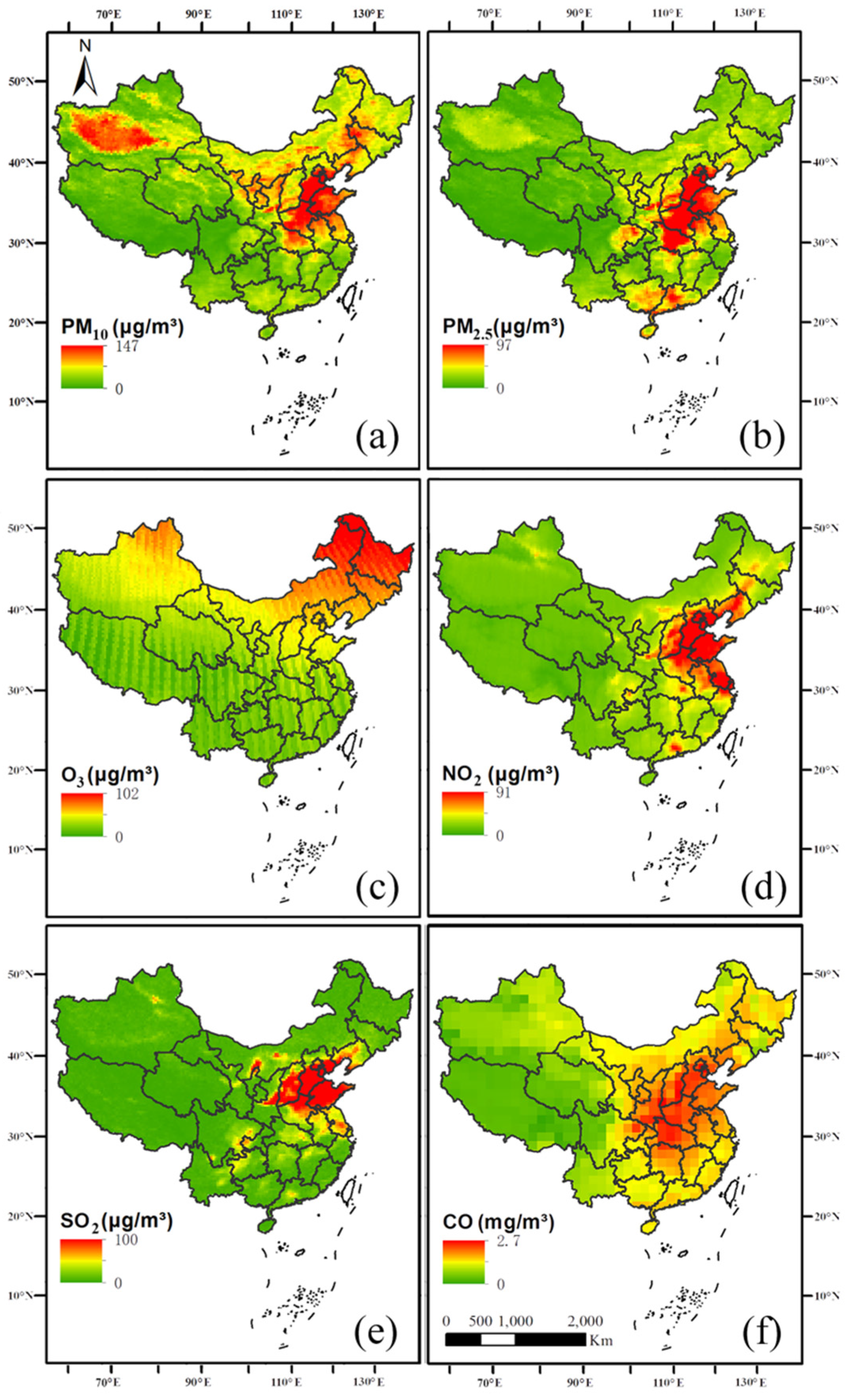
3.1. Spatial Distribution of Ambient Pollutant Concentrations

By using both satellite products and meteorological data, we derived the spatial distribution of six pollutants’ 10-year annual average concentration in China, as shown in Figure 2. The spatial resolution of the PM₁₀, PM_2.5, O₃, NO₂ and SO₂ maps is 0.25°× 0.25° and the CO map has a spatial resolution of 1° × 1°. It is clearly seen that PM₁₀ pollution in the northern regions was significantly heavier than in the southern regions. The highest PM₁₀ concentrations, with an average PM₁₀ concentration greater than 100 µg/m³, are located in eastern and northwest China. The scope of the serious pollution regions affected by PM_2.5 was more concentrated and mainly located in major industrial zones with a rapid economic development. Regions with high O₃ concentrations were located in northeast China. Regions with high NO₂ concentration were mainly situated in eastern coastal area. The SO₂ pollution seems very light in the whole country. The maximum 10-year annual average concentration of CO was 2.7 mg/m³, which was still lower than 4 mg/m³ required by ambient quality standards.

3.2. Spatial Distribution of Health Impact Attributed to Ambient Pollutants

The exposure-response function was applied together with population raster data to evaluating health impact and obtained the 10-year annual average health impact caused by each ambient pollutant, as showed in Figure 3. The spatial resolution of the PM₁₀, PM_2.5, O₃, NO₂ and SO₂ maps is 0.25°× 0.25° and the CO map has a spatial resolution of 1° × 1°. It has to be noted that the annual average concentrations of CO over the past decade are all below the threshold concentration we selected (Appendix A) and the excessive risk of CO almost decreased to zero. The value in the figure symbolized the overall health impact in each 0.25° × 0.25° grid (region). Generally, heavy health impact regions affected by PM₁₀ were located in eastern China, where population density was high and the concentration of PM₁₀ exceeds the threshold concentration seriously. The heaviest PM_2.5 pollution regions were surrounded by the eastern coastal area. As the O₃ concentrations generally follow a latitude distribution, the adverse effect caused by O₃ decreased from north to south in eastern China. In addition, the region influenced by NO₂ were much smaller and more concentrated. The region influenced by SO₂ were a little bigger than NO₂, which was mainly located at areas surrounding eastern China.

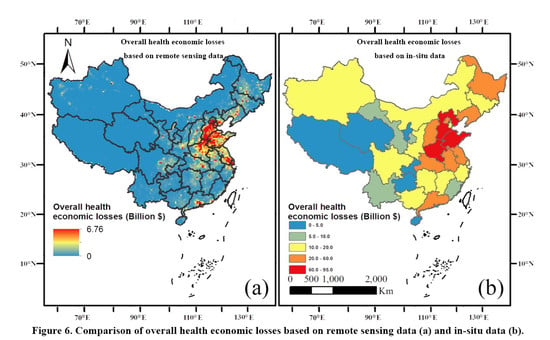
3.3. Spatial Distribution of Overall Health Economic Losses Caused by Ambient Pollutants

The AHC approach was employed to quantify health impact in terms of monetary value and the spatial distribution of 10-year annual average overall health economic losses from exposure to all ambient pollutants in China with the spatial resolution of 0.25° × 0.25° is given in Figure 4. Based on the definition of PM₁₀ and PM_2.5, direct addition may cause a double-counting issue [61], so we did not include PM_2.5 when we calculated the overall economic losses. It is seen that health economic losses showed a large spatial heterogeneity across China and roughly exhibited a decreasing trend from east to west. The most serious loss was 6.76 billion dollars /625 km², mainly distributed in eastern China. In addition to these concentrated patches, high-risk regions were distributed like scattered point and sporadic throughout other regions. However, western China had less health losses due to lower human density and less industrial pollution. By zonal statistical tool, we calculated the sum of economic losses of all regions in China and obtained the 10-year annual average overall health economic losses caused by six ambient pollutants, which is 283.80 billion US dollars and account for 4.05% of China’s total GDP.

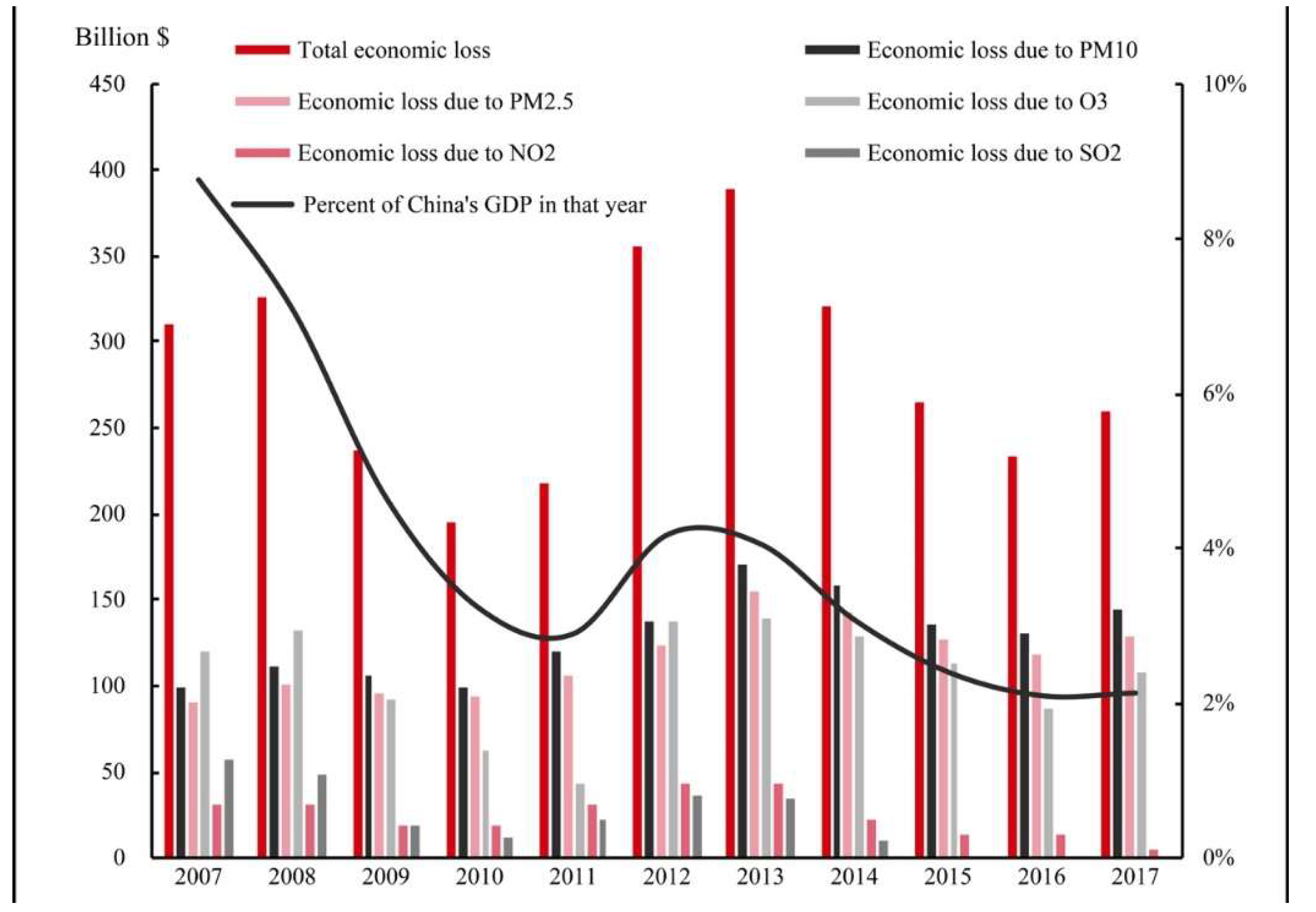
3.4. Historical Change of Overall Health Economic Losses Caused by Ambient Pollutants

In terms of historical changes, the overall health economic loss is volatile, reaching a record low in 2010 with a total loss of nearly $200 billion and a record high in 2013 with a total loss of nearly $400 billion, as showed in Figure 5. At the same time, the proportion of health economic losses in China’s GDP has been declining year by year, reaching a record high of 8.76% in 2007 and a record low of 2.13% in 2017. From the differences of economic losses caused by various pollutants, the severity of economic losses caused by pollutants is roughly shown as: PM₁₀ > PM_2.5 > O₃ > NO₂ > SO₂.

4. Discussion

4.1. Higher Spatial Resolution Contributes in Overall Economic Losses

Spatial assessment results based on higher spatial resolution of data source provided more detail of spatial information which revealed the spatial distribution and variance of health economic losses in various regions of China. In order to highlight the advantages of using higher spatial resolution in the refined assessment of health economic losses, we compared the results based on remote sensing data and in-situ data, as showed in Figure 6. It is clearly shown that the outcome of the conventional assessment method was only given in provincial level with missing sub-provincial variability details, as compared to the results from the improvement of spatial resolution of data source. The application of remote sensing and population raster data was the key of the map of human health impact, and finally provided the foundation for spatial assessment of health economic losses as a result of the degrading air quality.

Furthermore, spatial assessment of overall health economic losses is different from conventional result due to more detail spatial information. The above two kinds of historical results based on remote sensing data and in-situ data are computed with the zonally statistical method respectively to obtain overall economic losses from 2007 to 2017 in China, as shown in Figure 7.

Compared with the in-situ data (red line), health economic losses based on remote sensing data (black line) are apparently lower. One of the reasons is that monitoring stations may mainly clustered in zones of poor ambient quality and represent air quality at a particular location. As a result, the severity of health economic losses based on the big spatial resolution of data source which using the average value of in-situ data to represent the overall regional concentration could be over-estimated [11,12]. In other words, most of monitoring stations are located in the zones where concentrations of ambient pollutants are generally higher, so that using the in-situ data alone is likely to misrepresent the overall regional concentrations. On the other hand, the fact that geographical distribution of pollutants concentration and population density were often inconsistent was probably ignored in conventional assessment methods [15]. As usual, the regional average concentration was used to match total population in one province, but not everyone is exposed to the same pollutants concentration. In fact, the economic losses in highly polluted regions with very low population density are not definitely serious [62]. In the same way, the economic losses cannot be ignored in the regions where the concentration of pollution is relatively low but has large population density.

However, as we discuss in the next section, compared with ground-based measurements, the satellite-derived pollutant concentrations is generally understated. Therefore, to quantify the effect of pollutant underestimation to the overall difference seen in Figure 7, we applied the linear regressions in Figure 8 (in Section 4.2.1), which is derived over these 348 stations, to derive bias-corrected six ambient pollutants for each grid cell of satellite data over China from 2007 to 2017, to ensure that the bias-corrected satellite-derived pollutant concentrations over these 348 points are equal to in-situ data in these stations in terms of overall statistics, i.e., mean value. Note that variance from station to station exists. Then, with the method consistent with that in the manuscript, we estimated the economic losses based on the spatial distribution of bias-corrected satellite-derived concentration of six pollutants and it is shown as the yellow line in Figure 7, which is much closer to the black line. In addition, we applied the linear regressions in Figure 8 to derive a set of new annual average concentration of six ambient pollutants only over the 348 cities from 2007 to 2017, which are considered as the bias-corrected satellite-derived pollutant concentrations over these 348 points, which have in situ observations. Then, with the method consistent with that in the estimation of economic losses with in situ observations, we estimated the economic losses based on the bias-corrected satellite-derived concentration of six pollutants over the 348 stations and it is shown as the grey curve in Figure 7.

It is clearly shown that the underestimation in satellite-derived pollutant concentrations alone, i.e., the gap between yellow and black line, amounts to about 30% the difference between economic losses estimated from in-situ data and that from satellite-derived data, i.e., the gap between the red line and black line. The grey line is based on bias-corrected satellite data over the 348 stations, but preserved the same spatial distribution as in-situ data. Therefore, the gap between the red and gray line, which is also about 30%, is purely coming from the combined effect from the variance in the linear regressions in Figure 8.

The gap between the grey line and the yellow line can be considered as the contribution from the finer spatial resolution from satellite-derived concentration of pollutants, which is also amounts to about 30%. Therefore, underestimation of satellite-derived pollutant concentrations contributes about 1/3 of the overall difference in economic losses based on in-situ data vs. those based on satellite data, and another 1/3 is from the finer spatial resolution from both satellite data and population density data. The finer spatial resolution of remote sensing data may provide detailed spatial variability of assessment of overall economic impact from air pollutions, however, it should be noted that there are no grounds to state that the result based on linear regressions data (grey line or yellow line) or remote sensing data (black line) is closer to true value than the in-situ data (red line) under current research.

4.2. Uncertainty Analysis

4.2.1. Validation of Satellite-Derived Ambient Pollutant Concentrations

The precision and accuracy of satellite-derived ambient pollutant concentrations determines the uncertainties in estimation of health economic losses from exposure to ambient pollutants, but PM₁₀, PM_2.5, O₃, NO₂, SO₂, CO were not listed as the main air pollutants and monitored nationwide until 2013 in China. So, to estimate the accuracy of the satellite derived ambient pollutant concentrations, the 4-year annual average PM₁₀, PM_2.5, O₃, NO₂, SO₂, CO concentrations in 348 Chinese cities from 2014 to 2017 were collected as truth data, which were used to validate the 4-year annual average satellite-derived PM₁₀, PM_2.5, O₃, NO₂, SO₂, CO concentrations from 2014 to 2017. Note that, ambient pollutant concentrations in each city were the mean value of all the monitoring stations in both urban and sub-urban areas.

The correlation between satellite-retrieved and ground-based ambient pollutants concentrations is shown in Figure 8. In general, a great liner relationship exists between satellite-derived ambient pollutant concentrations and ground-based concentrations. The correlation coefficient between surface measurement PM₁₀, PM_2.5, NO₂, SO₂, CO, O₃ concentrations and corresponding satellite-derived concentrations can be as high as 0.70, 0.72, 0.73, 0.51, 0.52 and 0.45, respectively. The root mean square error (RMSE) is about 16.61, 9.19, 7.11, 3.24, 0.38 and 4.58. The p-value is about 0.0197, 0.0214, 0.0205, 0.0334, 0.0408 and 0.0081 (95%CI). High correlation and low RMSE indicates the applicability and reliability of ambient pollutant concentrations derived from satellite observations.

4.2.2. Uncertainty Analysis of Final Economic Losses Valuation

The uncertainty in satellite-derived ambient pollutant concentrations could be propagated to the final losses results. Firstly, the uncertainty influenced the number of deaths or illnesses of health endpoints caused by air pollution. Then, this uncertainty in health impact was propagated to economic losses valuation. However, quantifying the uncertainty of final losses results is not straightforward, it not only depends on the uncertainty in satellite-derived ambient pollutant concentrations, but also on other factors as described below.

First of all, there is an inter-correlation between ambient pollutants, which leads to the intersection and interaction of health economic losses caused by each pollutant. Simple and direct addition to obtain total health loss may cause over-counting issue. The correlation exists between the concentrations of six air pollutants, especially between PM₁₀ and PM_2.5, and the annual average concentrations of PM_2.5 and PM₁₀ are positively correlated with NO₂ and SO₂ [63], which are mainly related to the common pollution source and the photochemical reaction between ambient pollutants [64]. In this study, the overall health economic losses of the six pollutants were simply and directly added, it in generally leads to uncertainty in the direction of overestimation.

Secondly, the reference concentration $C_0$ of each ambient pollutant in Equation (7) is a sensitive parameter and affects the accuracy of the quantified economic loss. The reference concentration of pollutants directly determines the baseline of pollutant health impact assessment, but the selection of reference concentration is widely controversial. In researches conducted both in china and other part of world, it is indicated that finding a uniform threshold value is difficult. At the same time, due to the differences in tolerance and sensitivity of different races to the disease, there will also be large coefficient differences in different regions or at different time periods [56]. Therefore, the use of different standards will have a certain impact on the final economic loss valuation, however, the magnitude of the associated uncertainty is much smaller.

4.3. Potential for Spatial Assessment Based on Higher Spatial Resolution

Spatial assessment result based on higher spatial resolution of data source can reveal the spatial distribution and variance of health economic losses in various regions of China. The potential of spatial assessment for future application mainly include: Firstly, the high-risk regions affected by ambient pollutants of each administrative area can be determined to the county-level units and help to identify which pollutant have the greatest impact in this region, so that specific pollution control measures can be taken in a targeted manner. In addition, the comparison of historical assessment outcomes can be used for the evaluation of atmospheric governance results. This evaluation is not limited to the overall level, but a comprehensive evaluation of the various regions. Besides, accurate health economic losses are the raw input parameters for other economic loss assessments and provides the foundation for further losses accounting in other fields. This would help in obtaining more reasonable results so as to influence the formulation of further policies.

5. Conclusions

Air pollution has become a serious regional environmental issue in various regions of China and the harmful effects caused by ambient pollutants on human health are increasingly attracting public concern. To identify the spatial distribution of regions with heavy health economic losses caused by air pollution and help taking targeted pollution control measures for various regions, spatial assessment of health economic losses associated with ambient pollutants in China is indispensable. This study utilized the higher spatial resolution pollutants concentration and population raster data to spatially assess the corresponding health economic losses due to exposure to ambient pollutants. The results from this study presented the health economic losses from exposure to ambient pollutants in a spatial resolution of 0.25° × 0.25° and evaluated the health impact from air pollution at sub-provincial level. Compared with conventional assessment method based on in-situ data, higher spatial resolution data source could make some improvement. Spatial assessment result based on higher spatial resolution of data source provided more detail of spatial information which revealed the spatial distribution and variance of health economic losses in various regions of China. Furthermore, spatial assessment of overall health economic losses is different from conventional result due to more detail spatial information. However, it should be noted that it is difficult to draw the conclusion the result based on linear regressions data or remote sensing data is closer to true value than the in-situ data under current research, due to the uncertainties existed in the satellite-estimated surface-level concentration of pollutants.

Further studies should focus on applying remote sensing data with higher spatial resolution, in order to promote reliability and authenticity of satellite-derived pollutants concentration. Additionally, in the follow-up studies, the intersection and interaction between ambient pollutants on human health and economic losses should be fully considered. In addition, it’s necessary to focus on the range of use of the reference concentration in different regions or at different time points. Quantification of uncertainty in the estimation of economic losses needs to be further address in the future study.

References

1. Murray, J.L.C.; Vos, T.; Lozano, R.; Naghavi, M.; DFlaxman, A.; Michaud, C.; Ezzati, M.; Shibuya, K.; Salomon, J.; Abdalla, S.; et al. Disability-adjusted life years (DALYs) for 291 diseases and injuries in 21 regions, 1990–2010: A systematic analysis for the global burden of disease study 2010. Lancet 2012, 380, 2197–2223. [Google Scholar] [CrossRef]
2. Lu, X.; Lin, C.; Li, Y.; Yao, T.; Fung, J.C.; Lau, A.K. Assessment of health burden caused by particulate matter in southern China using high-resolution satellite observation. Environ. Int. 2017, 98, 160–170. [Google Scholar] [CrossRef] [PubMed]
3. Xia, Y.; Guan, D.B.; Jiang, X.J.; Peng, L.Q.; Schroeder, H.; Zhang, Q. Assessment of socioeconomic costs to China’s air pollution. Atmos. Environ. 2016, 139, 147–156. [Google Scholar] [CrossRef]
4. Wang, P.; Mu, H. Economic assessment on health loss of particulate air pollution in dalian of china. In Proceedings of the 2010 4th International Conference on Bioinformatics and Biomedical Engineering, Chengdu, China, 18–20 June 2010. [Google Scholar]
5. Turner, M.C.; Krewski, D.; Pope Iii, C.A.; Chen, Y.; Gapstur, S.M.; Thun, M.J. Long-term ambient fine particulate matter air pollution and lung cancer in a large cohort of never-smokers. Am. J. Respir. Crit. Care Med. 2011, 184, 1374–1381. [Google Scholar] [CrossRef] [PubMed]
6. Michael, J. Long-term ozone exposure and mortality. N. Engl. J. Med. 2009, 11, 1085–1095. [Google Scholar] [CrossRef] [Green Version]
7. Raaschou-Nielsen, O.; Andersen, Z.J.; Beelen, R.; Samoli, E.; Stafoggia, M.; Weinmayr, G.; Hoffmann, B.; Fischer, P.; Nieuwenhuijsen, M.J.; Brunekreef, B.; et al. Air pollution and lung cancer incidence in 17 European cohorts:Prospective analyses from the European Study of Cohorts for Air Pollution Effects (ESCAPE). Lancet Oncol. 2013, 14, 813–822. [Google Scholar] [CrossRef]
8. Chen, R.J.; Samoli, E.; Wong, C.-M.; Huang, W.; Wang, Z.S.; Chen, B.H.; Kan, H.D. Associations between short-term exposure to nitrogen dioxide and mortality in 17 Chinese cities: The China Air Pollution and Health Effects Study (CAPES). Environ. Int. 2012, 45, 32–38. [Google Scholar] [CrossRef]
9. Bernstein, J.A.; Alexis, N.; Barnes, C.; Bernstein, I.L.; Nel, A.; Peden, D.; Diaz-Sanchez, D.; Tarlo, S.M.; Williams, P.B.; Bernstein, J.A. Health effects of air pollution. J. Allergy Clin. Immunol. 2004, 114, 1116–1123. [Google Scholar] [CrossRef]
10. Wang, W.; Yu, T.; Ciren, P.; Jiang, P. Assessment of human health impact from PM10 exposure in China based on satellite observations. J. Appl. Remote Sens. 2015, 9, 096027. [Google Scholar] [CrossRef] [Green Version]
11. Michael, B. Estimating long-term average particulate air pollution concentrations: Application of traffic indicators and geographic information systems. Epidemiology 2003, 2, 228–239. [Google Scholar] [CrossRef]
12. Wilson, W.E.; Suh, H.H. Fine particles and coarse particles: Concentration relationships relevant to epidemiologic studies. J. Air Waste Manage. Assoc. 1997, 12, 1238–1249. [Google Scholar] [CrossRef] [PubMed] [Green Version]
13. World Bank. Cost of Pollution in China: Economic Estimates of Physical Damages; World Bank: Washington, DC, USA, 2007. [Google Scholar]
14. Zhang, M.; Song, Y.; Cai, X. A health-based assessment of particulate air pollution in urban areas of Beijing in 2000–2004. Sci. Total Environ. 2007, 376, 100–108. [Google Scholar] [CrossRef] [PubMed]
15. Guan, Y.; Rong, B.; Wang, Y.; Li, X.; Xiong, S.G. Assessment and regional diversity analysis of public health lost attributed by PM2.5 exposure in China. Environ. Pollut. Control 2019, 41, 798–802. [Google Scholar] [CrossRef]
16. EARTHDATA Search. Available online: https://search.earthdata.nasa.gov (accessed on 11 December 2018).
17. OMI Team. Ozone Monitoring Instrument (OMI) Data User’s Guide; NASA: Washington, DC, USA, 2012.
18. Deeter, M. MOPITT (Measurements of Pollution in the Troposphere) Version 5 Product User’s Guide. National Center for Atmospheric Research 2011. Available online: https://www.acom.ucar.edu/mopitt/v5_users_guide_beta.pdf (accessed on 27 February 2020).
19. European Copernicus space program. Global Human Settlement Layer (GHSL) Dataset. Available online: https://ghslsys.jrc.ec.europa.eu/index.php (accessed on 28 January 2019).
20. Center for Health Statistics and Information. An Analysis Report of National Health Services Survey in China, Beijing, 2008. Available online: http://www.nhc.gov.cn/mohwsbwstjxxzx/s8211/201009/49165.shtml (accessed on 27 February 2020).
21. Center for Health Statistics and Information. An Analysis Report of National Health Services Survey in China, Beijing, 2013. Available online: http://www.nhc.gov.cn/mohwsbwstjxxzx/s8211/201610/9f109ff40e9346fca76dd82cecf419ce.shtml (accessed on 27 February 2020).
22. Ministry of Public Health. Chinese Yearbook of Health Statistics 2008–2018; People’s Health Press: Beijing, China, 2008. [Google Scholar]
23. World Bank. World Bank Open Data. Available online: https://data.worldbank.org/ (accessed on 30 January 2019).
24. National Meteorological Information Center. Available online: http://data.cma.cn/site/index.html (accessed on 18 December 2018).
25. Ministry of Ecology and Environmental Protection of the People’s Republic of China. Bulletin on China’s Ecological Environment 2007. Available online: http://www.mee.gov.cn/hjzl/zghjzkgb/lnzghjzkgb/ (accessed on 20 January 2019).
26. Koelemeijer, R.B.A.; Homan, C.D.; Matthijsen, J. Comparison of spatial and temporal variations of aerosol optical thickness and particulate matter over Europe. Atmos. Environ. 2006, 40, 5304–5315. [Google Scholar] [CrossRef]
27. Lin, C.Q.; Li, Y.; Yuan, Z.B.; Lau, A.K.H.; Li, C.C.; Fung, J.C.H. Using satellite remote sensing data to estimate the high-resolution distribution of ground-level PM2.5. Remote Sens. Environ. 2015, 156, 117–128. [Google Scholar] [CrossRef]
28. Yu, T.; Wang, W.; Ciren, P.; Zhu, Y. Assessment of human health impact from exposure to multiple air pollutants in China based on satellite observations. Int. J. Appl. Earth Obs. Geoinf. 2016, 52, 542–553. [Google Scholar] [CrossRef]
29. Zhang, B.; Zhang, M.; Kang, J.; Hong, D.; Xu, J.; Zhu, X. Estimation of PMx Concentrations from Landsat 8 OLI Images Based on a Multilayer Perceptron Neural Network. Remote Sens. 2019, 11, 646. [Google Scholar] [CrossRef] [Green Version]
30. Cheng, Z.; Ma, X.; He, Y.; Jiang, J.; Wang, X.; Wang, Y.; Sheng, L.; Hu, J.; Yan, N. Mass extinction efficiency and extinction hygroscopicity of ambient PM2.5 in urban China. Environ. Res. 2017, 156, 239–246. [Google Scholar] [CrossRef]
31. Im, J.-S.; Saxena, V.K.; Wenny, B.N. An assessment of hygroscopic growth factors for aerosols in the surface boundary layer for computing direct radiative forcing. J. Geophys. Res. Atmos. 2001, 106, 20213–20224. [Google Scholar] [CrossRef]
32. Bedoya-Velásquez, A.E.; Titos, G.; Bravo-Aranda, J.A.; Haeffelin, M.; Favez, O.; Petit, J.E.; Alados-Arboledas, L. Long-term aerosol optical hygroscopicity study at the ACTRIS SIRTA observatory: Synergy between ceilometer and in situ measurements. Atmos. Chem. Phys. 2019, 19, 7883–7896. [Google Scholar] [CrossRef] [Green Version]
33. Fernández, A.J.; Apituley, A.; Veselovskii, I.; Suvorina, A.; Henzing, J.; Pujadas, M.; Artíñano, B. Study of aerosol hygroscopic events over the Cabauw experimental site for atmospheric research (CESAR) using the multi-wavelength Raman lidar Caeli. Atmos. Environ. 2015, 120, 484–498. [Google Scholar] [CrossRef]
34. Boersma, K.F.; Jacob, D.J.; Trainic, M.; Rudich, Y.; DeSmedt, I.; Dirksen, R.; Eskes, H.J. Validation of urban NO2 concentrations and their diurnal and seasonal variations observed from the SCIAMACHY and OMI sensors using in situ surface measurements in Israeli cities. Atmos. Chem. Phys. 2009, 9, 3867–3879. [Google Scholar] [CrossRef] [Green Version]
35. Ding, Y.; Peng, L.; Ran, L.; Zhao, C.S. A method of inferring ground level NO2 using satellite-borne OMI observations. Acta Sci. Nat. Univ. Pekin. 2011, 47, 671–676. [Google Scholar] [CrossRef]
36. Gu, J.B.; Chen, L.F.; Yu, C.; Li, S.S.; Tao, J.H.; Fan, M.; Xiong, X.Z.; Wang, Z.F.; Shang, H.Z.; Su, L. Ground-level NO2 concentrations over China inferred from the satellite OMI and CMAQ model simulations. Remote Sens. 2017, 9, 519. [Google Scholar] [CrossRef] [Green Version]
37. Wang, Y.; Tao, J.; Cheng, L.; Yu, C.; Wang, Z.; Chen, L. A Retrieval of Glyoxal from OMI over China: Investigation of the Effects of Tropospheric NO2. Remote Sens. 2019, 11, 137. [Google Scholar] [CrossRef] [Green Version]
38. Yuchechen, A.; Lakkis, S.; Canziani, P. Linear and non-linear trends for seasonal NO2 and SO2 concentrations in the Southern Hemisphere (2004−2016). Remote Sens. 2017, 9, 891. [Google Scholar] [CrossRef] [Green Version]
39. Stull, R.B. An Introduction to Boundary Layer Meteorology; Springer: Berlin/Heidelberg, Germany, 2012. [Google Scholar]
40. Liu, S.; Liang, X.Z. Observed diurnal cycle climatology of planetary boundary layer height. J. Clim. 2010, 23, 5790–5809. [Google Scholar] [CrossRef]
41. University of Cambridge. Dobson Unit-Definition. Available online: http://www.atm.ch.cam.ac.uk/tour/dobson.html (accessed on 30 January 2019).
42. Wang, Z.J.; Chen, S.B.; Lv, H.; Han, N.L. Conversion on different dimensions of atmospheric ozone. J. Meteorol. Environ. 2010, 26, 63–67. [Google Scholar]
43. Fox, R.F.; Hill, T.P.; Fox, R.M. Macroscope: An Exact Value for Avogadro’s Number. Am. Sci. 2007, 95, 104–107. [Google Scholar] [CrossRef]
44. Hou, Q.; An, X.; Wang, Y.; Tao, Y.; Sun, Z. An assessment of China’s PM10-related health economic losses in 2009. Sci. Total Environ. 2012, 435–436, 61–65. [Google Scholar] [CrossRef]
45. Chen, C.H.; Chen, B.H.; Wang, B.Y.; Huang, C.; Zhao, J.; Dai, Y.; Kan, H.D. Low-carbon energy policy and ambient air pollution in Shanghai, China: A health-based economic assessment. Sci. Total Environ. 2007, 373, 13–21. [Google Scholar] [CrossRef] [PubMed]
46. Gao, J.L.; Yuan, Z.W.; Liu, X.W.; Xia, X.M.; Huang, X.J.; Dong, Z.F. Improving air pollution control policy in China-A perspective based on cost–benefit analysis. Sci. Total Environ. 2016, 543, 307–314. [Google Scholar] [CrossRef] [PubMed]
47. Voorhees, A.S.; Wang, J.D.; Wang, C.C.; Zhao, B.; Wang, S.X.; Kan, H.D. Public health benefits of reducing air pollution in Shanghai: A proof-of-concept methodology with application to BenMAP. Sci. Total Environ. 2014, 485–486, 396–405. [Google Scholar] [CrossRef] [PubMed]
48. Kumar, A.; Gupta, I.; Brandt, J.; Kumar, R.; Dikshit, A.K.; Patil, R.S. Air quality mapping using GIS and economic evaluation of health impact for Mumbai City, India. J. Air Waste Manag. Assoc. 2016, 66, 470–481. [Google Scholar] [CrossRef] [PubMed] [Green Version]
49. World Health Organization. WHO Air Quality Guidelines for Particulate Matter, Ozone, Nitrogen Dioxide and Sulfur Dioxide; WHO: Geneva, Switzerland, 2005. [Google Scholar]
50. World Health Organization. Air quality guidelines for Europe; WHO: Geneva, Switzerland, 2000. [Google Scholar]
51. Ambient Ambient Quality Standards. Available online: https://www.transportpolicy.net/standard/china-air-quality-standards/ (accessed on 27 February 2020).
52. Brajer, V.; Mead, R.W.; Xiao, F. Valuing the health impacts of air pollution in Hong Kong. J. Asian Econ. 2006, 17, 85–102. [Google Scholar] [CrossRef]
53. Hooper, L.G.; Young, M.T.; Keller, J.P.; Szpiro, A.A.; O’Brien, K.M.; Sandler, D.P.; Vedal, S.; Kaufman, J.D.; London, S.J. Ambient air pollution and chronic bronchitis in a cohort of U.S. women. Environ. Health Perspect. 2018, 126, 027005. [Google Scholar] [CrossRef]
54. Cui, J.; Yin, P.; Wang, L.J.; Liu, S.W.; Li, Y.C.; Liu, Y.N.; Liu, J.M.; You, J.L.; Zeng, X.Y.; Zhou, M.G. Burden of chronic obstructive pulmonary disease attributable to ambient ozone pollution in 1990 and 2013 in China. Zhonghua Yu Fang Yi Xue Za Zhi 2016, 50, 391–396. [Google Scholar] [CrossRef]
55. Lv, L.Y.; Li, H.Y. Health economic evaluation of PM10 and PM2.5 pollution in Beijing-Tianjin-Hebei region of China. Acta Sci. Nat. Univ. Nankaiensis 2016, 49, 69–77. [Google Scholar]
56. Zhong, M.T.; Shi, H.; Wang, H.X.; Yang, Z.; Zuo, N. Meta-analysis of air pollutant exposure-response relationship and its application in health impact assessment of exposure to air pollutants in Xi’an. Environ. Sci. Technol. 2017, 40, 171–178. [Google Scholar] [CrossRef]
57. Chen, B.H.; Hong, C.j.; Zhu, H.G. Quantitative evaluation of the impact of air sulfur dioxide on human health in the urban districts of shanghai. J. Environ. Health 2002, 19, 11–13. [Google Scholar] [CrossRef]
58. Zhao, B.; Wang, S.; Ding, D.; Wu, W.; Chang, X.; Wang, J.; Xing, J.; Jang, C.; Fu, J.S.; Zhu, Y. Nonlinear relationships between air pollutant emissions and PM2.5-related health impacts in the Beijing-Tianjin-Hebei region. Sci. Total Environ. 2019, 661, 375–385. [Google Scholar] [CrossRef] [PubMed]
59. Han, M.X.; Guo, X.M.; Zhang, Y.S. The human capital loss of air pollution in cities, China. China Environ. Sci. 2006, 26, 509–512. [Google Scholar] [CrossRef]
60. Ni, Z.Z. Health Statistics, 4th ed.; People’s Medical Publishing House: Beijing, China, 2000. [Google Scholar]
61. Lu, X.; Yao, T.; Fung, J.C.H.; Lin, C. Estimation of health and economic costs of air pollution over the Pearl River Delta region in China. Sci. Total Environ. 2016, 566–567, 134–143. [Google Scholar] [CrossRef] [PubMed] [Green Version]
62. Zeng, X.G.; Ran, F.F.; Peng, Y.Y. Health effects’ spatial distribution analysis of PM2.5 pollution in China based on spatial grid scale. China Environ. Sci. 2019, 39, 2624–2632. [Google Scholar]
63. Song, C.; Wu, L.; Xie, Y.; He, J.; Chen, X.; Wang, T.; Dai, Q. Air pollution in China: Status and spatiotemporal variations. Environ. Pollut. 2017, 227, 334–347. [Google Scholar] [CrossRef]
64. Xu, Y.; Ying, Q.; Hu, J.; Gao, Y.; Yang, Y.; Wang, D.; Zhang, H. Spatial and temporal variations in criteria air pollutants in three typical terrain regions in Shaanxi, China, during 2015. Air Qual. Atmos. Health 2018, 95–109. [Google Scholar] [CrossRef]
Figure 1. Flow chart of spatial assessment of health economic losses.
Remotesensing 12 00790 g001
Figure 2. Spatial distribution of 10-year annual average ambient pollutants concentration in China: (a) PM10; (b) PM2.5; (c) O3; (d) NO2; (e) SO2; (f) CO.
Remotesensing 12 00790 g002
Figure 3. Spatial distribution of 10-year annual average health impact caused by each ambient pollutant in China: (a) PM10; (b) PM2.5; (c) O3; (d) NO2; (e) SO2; (f) CO.
Remotesensing 12 00790 g003
Figure 4. Spatial distribution of 10-year annual average health economic losses from exposure to six ambient pollutants in China.
Remotesensing 12 00790 g004
Figure 5. Historical change of overall health economic losses caused by ambient pollutants in China.
Remotesensing 12 00790 g005
Figure 6. Overall health economic losses based on remote sensing data (a) and in-situ data (b).
Remotesensing 12 00790 g006
Figure 7. Comparison of economic losses based on in-situ data, remote sensing data and linear regressions data (348 points and spatial distribution).
Remotesensing 12 00790 g007
Figure 8. The correlation between satellite-retrieved and ground-based pollutants concentrations.
Remotesensing 12 00790 g008aRemotesensing 12 00790 g008b