Estimation of Hourly Rainfall during Typhoons Using Radar Mosaic-Based Convolutional Neural Networks


Abstract
:
1. Introduction
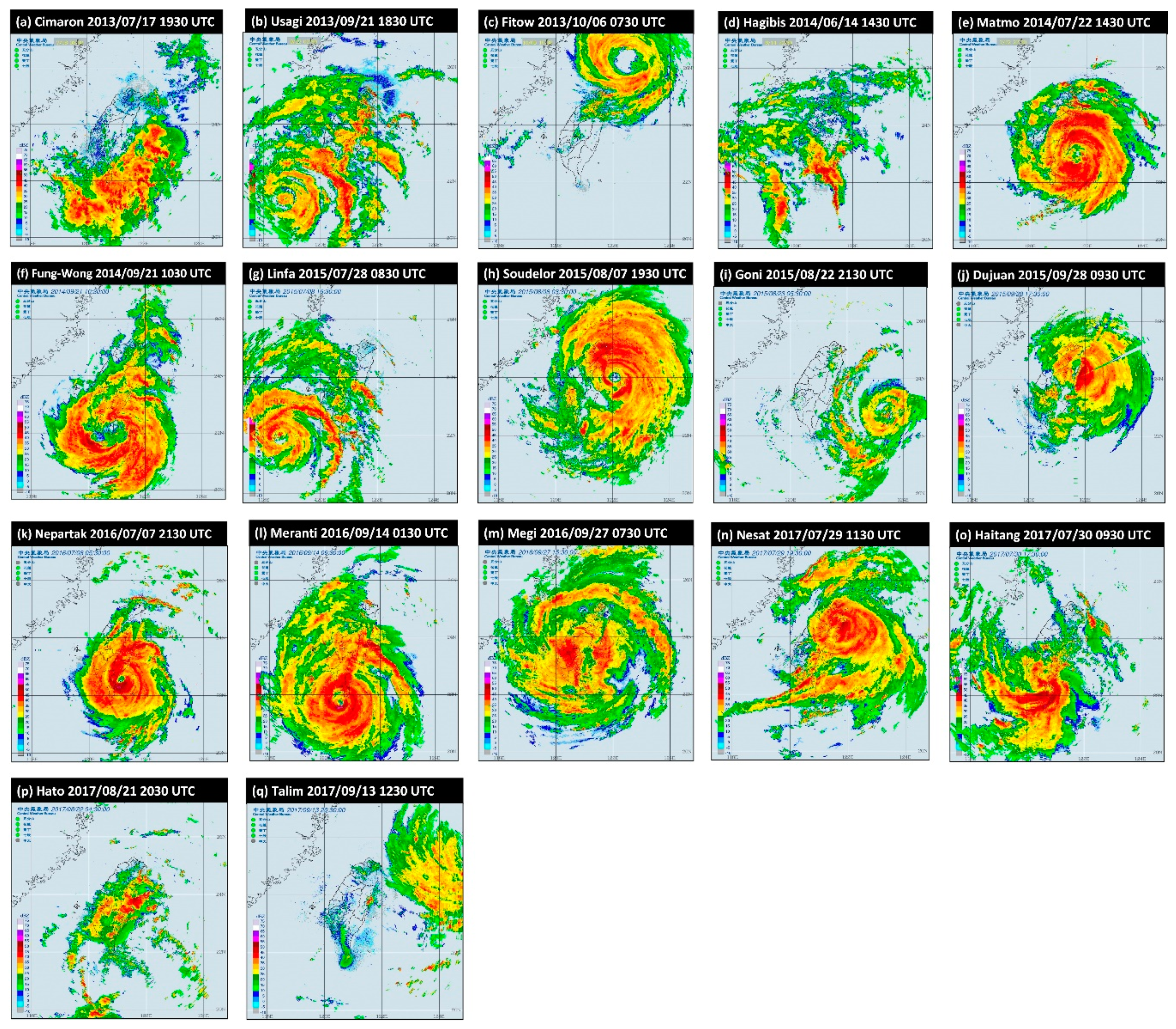
2. Materials
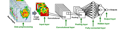
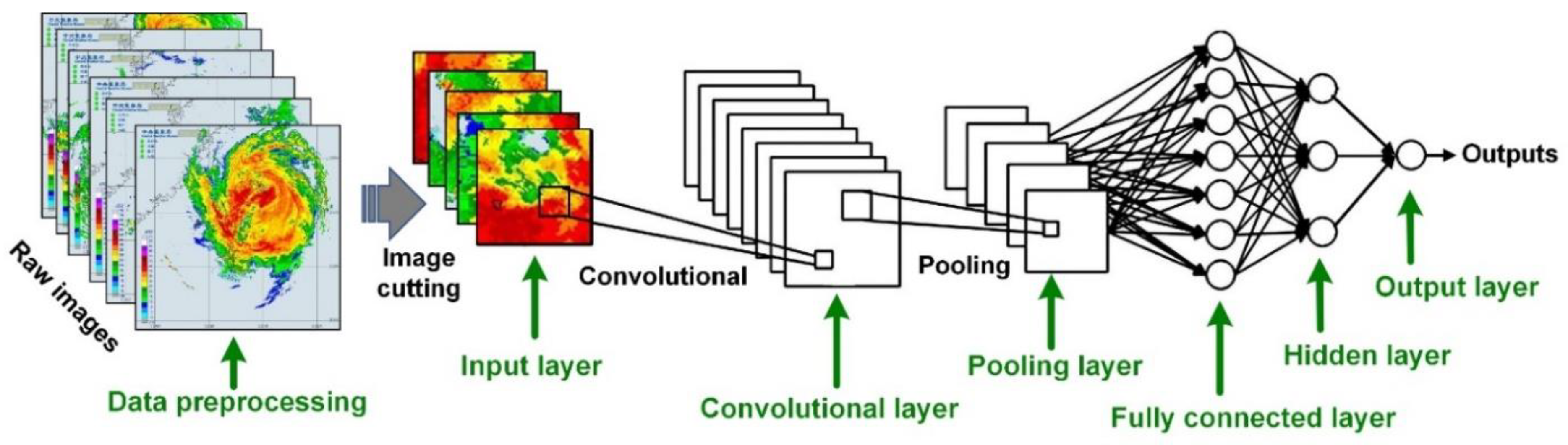
3. Methodology
Network Architecture
4. Modeling
4.1. Image Resizing and Selection
4.2. Parameter Calibration
5. Results and Discussion
5.1. Simulation Results
5.2. Evaluations
5.3. Estimation Performance for Peak Rainfall
6. Conclusions
Author Contributions
Funding
Acknowledgments
Conflicts of Interest
References
- Hsiao, L.H.; Peng, M.S.; Chen, D.S.; Huang, K.N.; Yeh, T.C. Sensitivity of typhoon track predictions in a regional prediction system to initial and lateral boundary conditions. J. Appl. Meteorol. Climatol. 2009, 48, 1913–1928. [Google Scholar] [CrossRef]
- Wei, C.C. Examining El Niño–Southern Oscillation effects in the subtropical zone to forecast long-distance total rainfall from typhoons: A case study in Taiwan. J. Atmos. Ocean. Technol. 2017, 34, 2141–2161. [Google Scholar] [CrossRef]
- Central Weather Bureau (CWB). Available online: http://www.cwb.gov.tw/V7/index.htm (accessed on 1 June 2019).
- Wang, M.; Zhao, K.; Xue, M.; Zhang, G.; Liu, S.; Wen, L.; Chen, G. Precipitation microphysics characteristics of a Typhoon Matmo (2014) rainband after landfall over eastern China based on polarimetric radar observations. J. Geophys. Res. Atmos. 2016, 121, 12415–12433. [Google Scholar] [CrossRef]
- Wei, C.C.; You, G.J.Y.; Chen, L.; Chou, C.C.; Roan, J. Diagnosing rain occurrences using passive microwave imagery: A comparative study on probabilistic graphical models and “black box” models. J. Atmos. Ocean. Technol. 2015, 32, 1729–1744. [Google Scholar] [CrossRef]
- Wei, C.C. Surface wind nowcasting in the Penghu Islands based on classified typhoon tracks and the effects of the Central Mountain Range of Taiwan. Weather Forecast. 2014, 29, 1425–1450. [Google Scholar] [CrossRef]
- Huang, C.Y.; Chou, C.W.; Chen, S.H.; Xie, J.H. Topographic rainfall of tropical cyclones past a mountain range as categorized by idealized simulations. Weather Forecast. 2020, 35, 25–49. [Google Scholar] [CrossRef]
- Wu, C.C.; Kuo, Y.H. Typhoons affecting Taiwan: Current understanding and future challenges. Bull. Am. Meteorol. Soc. 1999, 80, 67–80. [Google Scholar] [CrossRef]
- Fang, X.; Kuo, Y.H.; Wang, A. The impacts of Taiwan topography on the predictability of Typhoon Morakot’s record-breaking rainfall: A high-resolution ensemble simulation. Weather Forecast. 2011, 26, 613–633. [Google Scholar] [CrossRef] [Green Version]
- Hsiao, L.F.; Yang, M.J.; Lee, C.S.; Kuo, H.-C.; Shih, D.-S.; Tsai, C.-C.; Wang, C.-J.; Chang, L.-Y.; Feng, L.; Chen, D.-S.; et al. Ensemble forecasting of typhoon rainfall and floods over a mountainous watershed in Taiwan. J. Hydrol. 2013, 506, 55–68. [Google Scholar] [CrossRef] [Green Version]
- Huang, C.Y.; Chen, C.A.; Chen, S.H.; Nolan, D.S. On the upstream track deflection of tropical cyclones past a mountain range: Idealized experiments. J. Atmos. Sci. 2016, 73, 3157–3180. [Google Scholar] [CrossRef] [Green Version]
- Wu, C.C.; Yen, T.H.; Kuo, Y.H.; Wang, W. Rainfall simulation associated with Typhoon Herb (1996) near Taiwan. Part I: The topographic effect. Weather Forecast. 2002, 17, 1001–1015. [Google Scholar] [CrossRef]
- Wu, C.C.; Chou, K.H.; Lin, P.H.; Aberson, S.; Peng, M.; Nakazawa, T. Impact of dropwindsonde data on typhoon track forecasts in DOTSTAR. Weather Forecast. 2007, 22, 1157–1176. [Google Scholar] [CrossRef] [Green Version]
- Tsai, H.C.; Lee, T.H. Maximum covariance analysis of typhoon surface wind and rainfall relationships in Taiwan. J. Appl. Meteorol. Climatol. 2009, 48, 997–1016. [Google Scholar] [CrossRef]
- Wei, C.C. Improvement of typhoon precipitation forecast efficiency by coupling SSM/I microwave data with climatologic characteristics and precipitation. Weather Forecast. 2013, 28, 614–630. [Google Scholar] [CrossRef]
- Fabry, F.; Meunier, V.; Treserras, B.P.; Cournoyer, A.; Nelson, B. On the climatological use of radar data mosaics: Possibilities and challenges. Bull. Am. Meteorol. Soc. 2017, 98, 2135–2148. [Google Scholar] [CrossRef] [Green Version]
- Fabry, F. Radar Meteorology—Principles and Practice; Cambridge University Press: Cambridge, UK, 2015; p. 272. [Google Scholar]
- Marshall, J.M.; Palmer, W.M.K. The distribution of raindrops with size. J. Appl. Meteorol. 1948, 5, 165–166. [Google Scholar] [CrossRef]
- Biswas, S.K.; Chandrasekar, V. Cross-validation of observations between the GPM dual-frequency precipitation radar and ground based dual-polarization radars. Remote Sens. 2018, 10, 1773. [Google Scholar] [CrossRef] [Green Version]
- Georgakakos, K.P. Covariance propagation and updating in the context of real-time radar data assimilation by quantitative precipitation forecast models. J. Hydrol. 2000, 239, 115–129. [Google Scholar] [CrossRef]
- Hazenberg, P.; Torfs, P.J.J.F.; Leijnse, H.; Delrieu, G.; Uijlenhoet, R. Identification and uncertainty estimation of vertical reflectivity profiles using a Lagrangian approach to support quantitative precipitation measurements by weather radar. J. Geophys. Res. 2013, 118, 10243–10261. [Google Scholar] [CrossRef]
- Ivanov, S.; Michaelides, S.; Ruban, I. Mesoscale resolution radar data assimilation experiments with the harmonie model. Remote Sens. 2018, 10, 1453. [Google Scholar] [CrossRef] [Green Version]
- Krajewski, W.F.; Smith, J.A. Radar hydrology: Rainfall estimation. Adv. Water Resour. 2002, 25, 1387–1394. [Google Scholar] [CrossRef]
- Mimikou, M.A.; Baltas, E.A. Flood forecasting based on radar rainfall measurements. J. Water Resour. Plan. Manag. 1996, 122, 151–156. [Google Scholar] [CrossRef]
- Woo, W.C.; Wong, W.K. Operational application of optical flow techniques to radar-based rainfall. Nowcasting. Atmosphere 2017, 8, 48. [Google Scholar] [CrossRef] [Green Version]
- Ku, J.M.; Yoo, C. Calibrating radar data in an orographic setting: A case study for the typhoon Nakri in the Hallasan Mountain, Korea. Atmosphere 2017, 8, 250. [Google Scholar] [CrossRef] [Green Version]
- Libertino, A.; Allamano, P.; Claps, P.; Cremonini, R.; Laio, F. Radar estimation of intense rainfall rates through adaptive calibration of the Z-R relation. Atmosphere 2015, 6, 1559–1577. [Google Scholar] [CrossRef] [Green Version]
- Tang, J.; Matyas, C. A nowcasting model for tropical cyclone precipitation regions based on the TREC motion vector retrieval with a semi-Lagrangian scheme for doppler weather radar. Atmosphere 2018, 9, 200. [Google Scholar] [CrossRef] [Green Version]
- Chen, B.; Chen, B.; Lin, H.; Elsberry, R.L. Estimating tropical cyclone intensity by satellite imagery utilizing convolutional neural networks. Weather Forecast. 2019, 34, 447–465. [Google Scholar] [CrossRef]
- Kashiwao, T.; Nakayama, K.; Ando, S.; Ikeda, K.; Lee, M.; Bahadori, A. A neural network-based local rainfall prediction system using meteorological data on the Internet: A case study using data from the Japan Meteorological Agency. Appl. Soft Comput. 2017, 56, 317–330. [Google Scholar] [CrossRef]
- Lin, F.R.; Wu, N.J.; Tsay, T.K. Applications of cluster analysis and pattern recognition for typhoon hourly rainfall forecast. Adv. Meteorol. 2017, 2017, 17. [Google Scholar] [CrossRef]
- Lo, D.C.; Wei, C.C.; Tsai, N.P. Parameter automatic calibration approach for neural-network-based cyclonic precipitation forecast models. Water 2015, 7, 3963–3977. [Google Scholar] [CrossRef] [Green Version]
- Song, Y.; Han, D.; Rico-Ramirez, M.A. High temporal resolution rainfall rate estimation from rain gauge measurements. J. Hydroinform. 2017, 19, 930–941. [Google Scholar] [CrossRef] [Green Version]
- Unnikrishnan, P.; Jothiprakash, V. Data-driven multi-time-step ahead daily rainfall forecasting using singular spectrum analysis-based data pre-processing. J. Hydroinform. 2018, 20, 645–667. [Google Scholar] [CrossRef]
- Wei, C.C. Soft computing techniques in ensemble precipitation nowcast. Appl. Soft Comput. 2013, 13, 793–805. [Google Scholar] [CrossRef]
- Tripathi, S.; Srinivas, V.V.; Nanjundiah, R.S. Downscaling of precipitation for climate change scenarios: A support vector machine approach. J. Hydrol. 2006, 330, 621–640. [Google Scholar] [CrossRef]
- Wei, C.C. Meta-heuristic Bayesian networks retrieval combined polarization corrected temperature and scattering index for precipitations. Neurocomputing 2014, 136, 71–81. [Google Scholar] [CrossRef]
- Wei, C.C. Simulation of operational typhoon rainfall nowcasting using radar reflectivity combined with meteorological data. J. Geophys. Res. Atmos. 2014, 119, 6578–6595. [Google Scholar] [CrossRef]
- Tao, Y.; Gao, X.; Ihler, A.; Sorooshian, S.; Hsu, K. Precipitation identification with bispectral satellite information using deep learning approaches. J. Hydrometeorol. 2017, 18, 1271–1283. [Google Scholar] [CrossRef]
- Castelluccio, M.; Poggi, G.; Sansone, C.; Verdoliva, L. Land use classification in remote sensing images by convolutional neural networks. arXiv 2015, arXiv:1508.00092. [Google Scholar]
- Liu, Y.; Zhong, Y.; Fei, F.; Zhu, Q.; Qin, Q. Scene classification based on a deep random-scale stretched convolutional neural network. Remote Sens. 2018, 10, 444. [Google Scholar] [CrossRef] [Green Version]
- Marmanis, D.; Datcu, M.; Esch, T.; Stilla, U. Deep learning earth observation classification using ImageNet pretrained networks. IEEE Geosci. Remote Sens. Lett. 2016, 13, 105–109. [Google Scholar] [CrossRef] [Green Version]
- Nogueira, K.; Penatti, O.A.B.; dos Santos, J.A. Towards better exploiting convolutional neural networks for remote sensing scene classification. Pattern Recognit. 2017, 61, 539–556. [Google Scholar] [CrossRef] [Green Version]
- Tomè, D.; Monti, F.; Baroffio, L.; Bondi, L.; Tagliasacchi, M.; Tubaro, S. Deep convolutional neural networks for pedestrian detection. Signal Process. Image Commun. 2016, 47, 482–489. [Google Scholar] [CrossRef] [Green Version]
- Ronneberger, O.; Fischer, P.; Brox, T. U-Net: Convolutional networks for biomedical image segmentation. arXiv 2015, arXiv:1505.04597. [Google Scholar]
- Wu, H.; Gu, X. Towards dropout training for convolutional neural networks. Neural Netw. 2015, 71, 1–10. [Google Scholar] [CrossRef] [Green Version]
- Simonyan, K.; Zisserman, A. Very deep convolutional networks for large-scale image recognition. In Proceedings of the 2015 International Conference on Learning Representations (ICLR), San Diego, CA, USA, 7–9 May 2015; pp. 1–14. [Google Scholar]
- Zhang, W.; Tang, P.; Zhao, L. Remote sensing image scene classification using CNN-CapsNet. Remote Sens. 2019, 11, 494. [Google Scholar] [CrossRef] [Green Version]
- Chen, Y.; Duan, J.; An, J.; Liu, H. Raindrop size distribution characteristics for tropical cyclones and meiyu-baiu fronts impacting Tokyo, Japan. Atmosphere 2019, 10, 391. [Google Scholar] [CrossRef] [Green Version]
- Tran, Q.K.; Song, S. Multi-channel weather radar echo extrapolation with convolutional recurrent neural networks. Remote Sens. 2019, 11, 2303. [Google Scholar] [CrossRef] [Green Version]
- Lee, J.; Im, J.; Cha, D.H.; Park, H.; Sim, S. Tropical cyclone intensity estimation using multi-dimensional convolutional neural networks from geostationary satellite data. Remote Sens. 2020, 12, 108. [Google Scholar] [CrossRef] [Green Version]
- Pedregosa, F.; Varoquaux, G.; Gramfort, A.; Michel, V.; Thirion, B.; Grisel, O.; Blondel, M.; Prettenhofer, P.; Weiss, R.; Dubourg, V.; et al. Scikit-learn: Machine learning in Python. J. Mach. Learn. Res. 2011, 12, 2825–2830. [Google Scholar]
- Chollet, F. Keras: Deep Learning Library for Theano and Tensorflow. 2015. Available online: https://keras.io/ (accessed on 1 October 2019).
- Kingma, D.P.; Ba, J.L. Adam: A method for stochastic optimization. arXiv 2014, arXiv:1412.6980. [Google Scholar]


| Typhoon | Period (UTC) | Intensity | Total rain (mm) | ||
|---|---|---|---|---|---|
| Hualien | Sun Moon Lake | Taichung | |||
| Cimaron | 17–18 July 2013 | Mild typhoon | 29 | 1 | 13 |
| Usagi | 21–22 September 2013 | Severe typhoon | 303 | 25 | 5 |
| Fitow | 5–6 October 2013 | Moderate typhoon | 59 | 5 | 2 |
| Hagibis | 15–16 June 2014 | Mild typhoon | 10 | 16 | 5 |
| Matmo | 22–23 July 2014 | Moderate typhoon | 334 | 240 | 95 |
| Fung-Wong | 19–22 September 2014 | Mild typhoon | 169 | 64 | 31 |
| Linfa | 7–9 July 2015 | Mild typhoon | 9 | 2 | 12 |
| Soudelor | 7–8 August 2015 | Moderate typhoon | 219 | 133 | 66 |
| Goni | 22–23 August 2015 | Severe typhoon | 269 | 5 | 12 |
| Dujuan | 28–29 September 2015 | Severe typhoon | 168 | 129 | 87 |
| Nepartak | 7–9 July 2016 | Severe typhoon | 309 | 23 | 12 |
| Meranti | 13–14 September 2016 | Severe typhoon | 323 | 52 | 19 |
| Megi | 27–28 September 2016 | Moderate typhoon | 399 | 98 | 76 |
| Nesat | 28–29 July 2017 | Moderate typhoon | 55 | 209 | 42 |
| Haitang | 30–31 July 2017 | Mild typhoon | 90 | 79 | 153 |
| Hato | 22–23 August 2017 | Moderate typhoon | 115 | 6 | 8 |
| Talim | 13–13 September 2017 | Moderate typhoon | 33 | 0 | 0 |
| Image size | 4 × 4 | 6 × 6 | 8 × 8 | 10 × 10 | 12 × 12 | 14 × 14 | 16 × 16 |
| RMSE (mm/h) | 3.776 | 3.773 | 3.659 | 4.285 | 3.449 | 4.263 | 4.813 |
| Image size | 18 × 18 | 20 × 20 | 22 × 22 | 24 × 24 | 26 × 26 | 28 × 28 | 30 × 30 |
| RMSE (mm/h) | 3.886 | 3.639 | 4.344 | 4.014 | 3.854 | 4.461 | 4.114 |
| Image size | 4 × 4 | 6 × 6 | 8 × 8 | 10 × 10 | 12 × 12 | 14 × 14 | 16 × 16 |
| RMSE (mm/h) | 3.473 | 3.787 | 3.273 | 3.447 | 3.343 | 3.061 | 3.330 |
| Image size | 18 × 18 | 20 × 20 | 22 × 22 | 24 × 24 | 26 × 26 | 28 × 28 | 30 × 30 |
| RMSE (mm/h) | 3.182 | 3.280 | 3.172 | 3.158 | 3.446 | 3.706 | 4.002 |
| Image size | 4 × 4 | 6 × 6 | 8 × 8 | 10 × 10 | 12 × 12 | 14 × 14 | 16 × 16 |
| RMSE (mm/h) | 2.797 | 2.997 | 3.061 | 2.662 | 2.478 | 2.640 | 2.534 |
| Image size | 18 × 18 | 20 × 20 | 22 × 22 | 24 × 24 | 26 × 26 | 28 × 28 | 30 × 30 |
| RMSE (mm/h) | 2.623 | 3.119 | 3.091 | 3.127 | 2.936 | 3.017 | 3.099 |
| Station | Model | RMCNN | RMMLP | Z-R_MP | Z-R_ station |
|---|---|---|---|---|---|
| Hualien | MAE (mm/h) | 1.870 | 2.218 | 2.670 | 4.206 |
| RMSE (mm/h) | 3.502 | 4.351 | 4.955 | 7.569 | |
| rMAE | 0.309 | 0.366 | 0.441 | 0.695 | |
| rRMSE | 0.579 | 0.719 | 0.818 | 1.250 | |
| r | 0.946 | 0.930 | 0.868 | 0.854 | |
| CE | 0.867 | 0.794 | 0.733 | 0.378 | |
| Sun Moon Lake | MAE (mm/h) | 1.070 | 1.340 | 1.522 | 2.268 |
| RMSE (mm/h) | 2.124 | 2.672 | 3.155 | 4.458 | |
| rMAE | 0.314 | 0.393 | 0.446 | 0.665 | |
| rRMSE | 0.623 | 0.783 | 0.925 | 1.307 | |
| r | 0.961 | 0.939 | 0.835 | 0.852 | |
| CE | 0.860 | 0.778 | 0.691 | 0.383 | |
| Taichung | MAE (mm/h) | 0.771 | 0.905 | 1.141 | 1.474 |
| RMSE (mm/h) | 1.641 | 1.828 | 2.361 | 2.836 | |
| rMAE | 0.440 | 0.517 | 0.651 | 0.842 | |
| rRMSE | 0.937 | 1.043 | 1.348 | 1.619 | |
| r | 0.878 | 0.843 | 0.655 | 0.741 | |
| CE | 0.727 | 0.661 | 0.416 | 0.185 |
© 2020 by the authors. Licensee MDPI, Basel, Switzerland. This article is an open access article distributed under the terms and conditions of the Creative Commons Attribution (CC BY) license (http://creativecommons.org/licenses/by/4.0/).
Share and Cite
Wei, C.-C.; Hsieh, P.-Y. Estimation of Hourly Rainfall during Typhoons Using Radar Mosaic-Based Convolutional Neural Networks. Remote Sens. 2020, 12, 896. https://doi.org/10.3390/rs12050896
Wei C-C, Hsieh P-Y. Estimation of Hourly Rainfall during Typhoons Using Radar Mosaic-Based Convolutional Neural Networks. Remote Sensing. 2020; 12(5):896. https://doi.org/10.3390/rs12050896
Chicago/Turabian StyleWei, Chih-Chiang, and Po-Yu Hsieh. 2020. "Estimation of Hourly Rainfall during Typhoons Using Radar Mosaic-Based Convolutional Neural Networks" Remote Sensing 12, no. 5: 896. https://doi.org/10.3390/rs12050896
APA StyleWei, C.-C., & Hsieh, P.-Y. (2020). Estimation of Hourly Rainfall during Typhoons Using Radar Mosaic-Based Convolutional Neural Networks. Remote Sensing, 12(5), 896. https://doi.org/10.3390/rs12050896