Retrieval and Validation of Water Turbidity at Metre-Scale Using Pléiades Satellite Data: A Case Study in the Gironde Estuary

Abstract
:
1. Introduction
2. Data and Methods
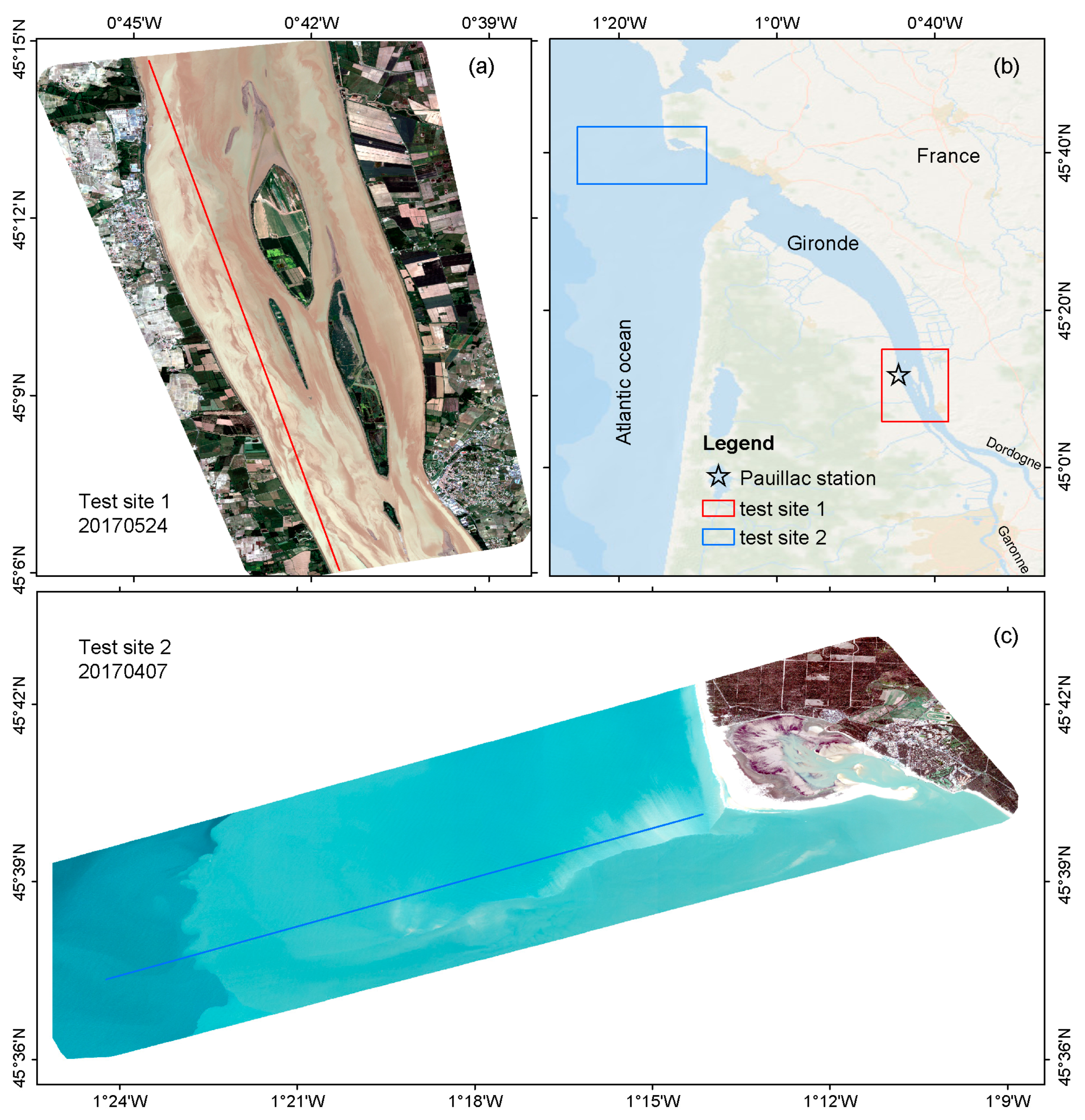
2.1. Study Area
2.2. Data Sets
2.2.1. Pléiades Imagery and DSF Atmospheric Correction
2.2.2. Landsat/OLI and MODIS Satellite Data
2.2.3. In Situ Measurements
2.3. Methods
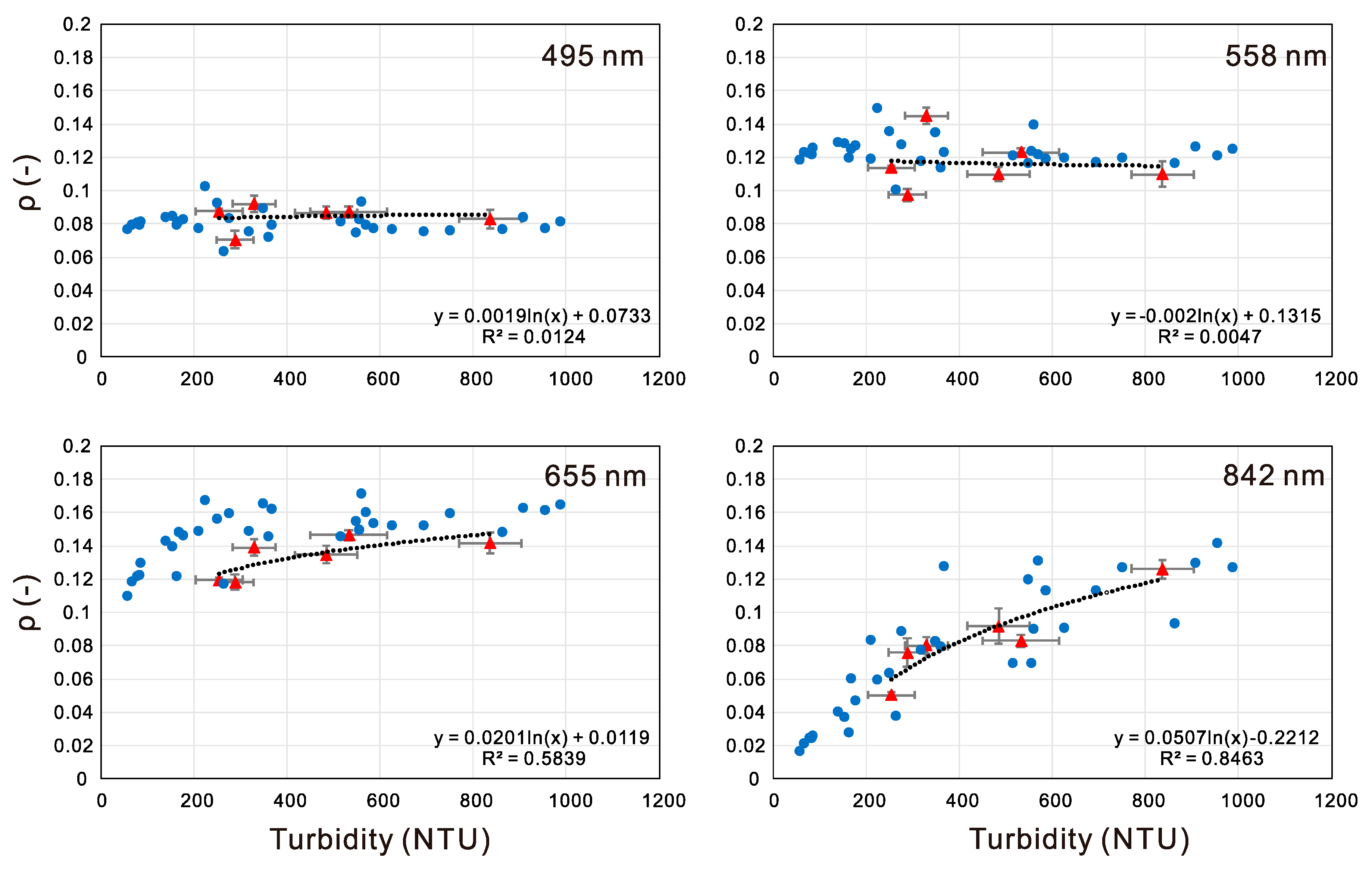
2.3.1. Calibration of Water Turbidity Algorithms
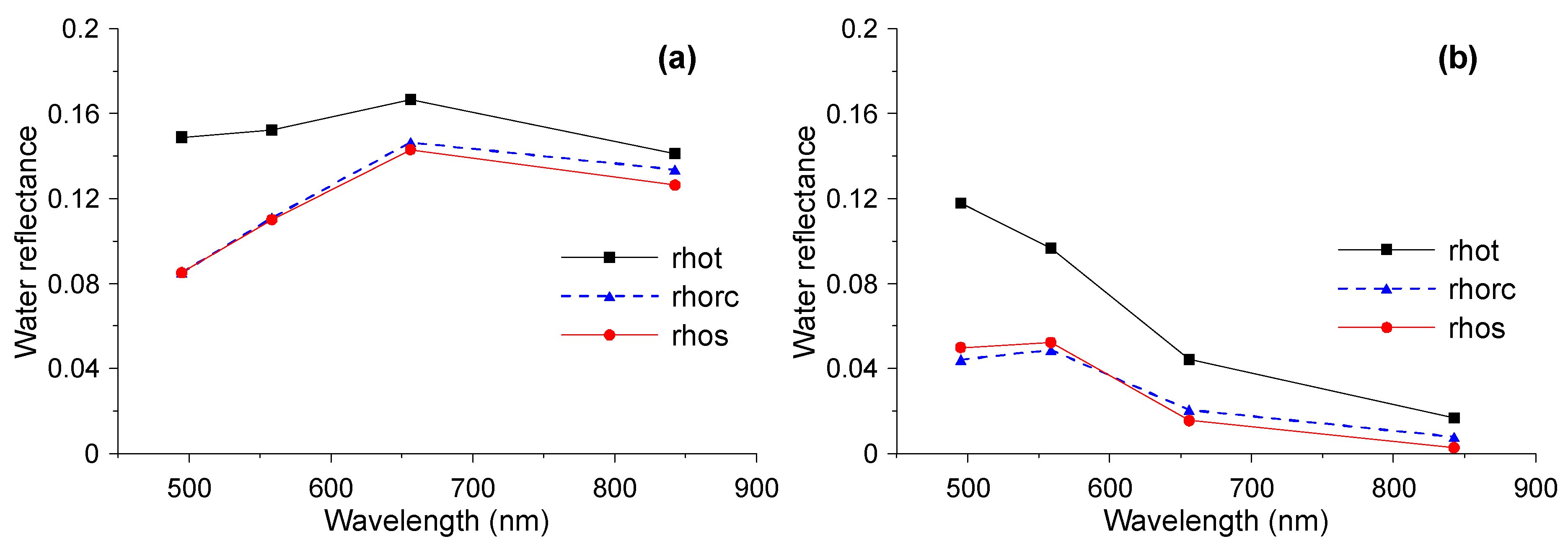
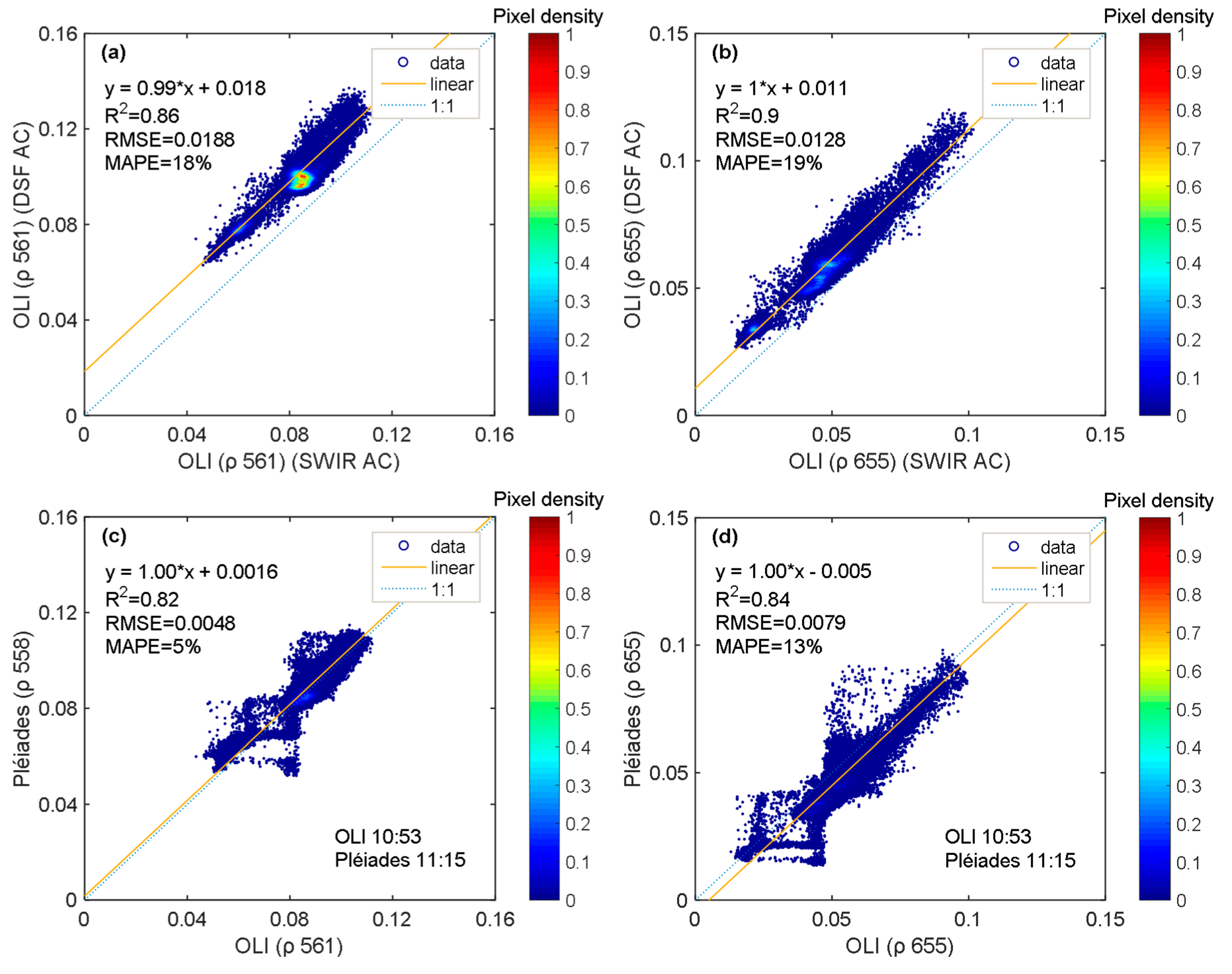
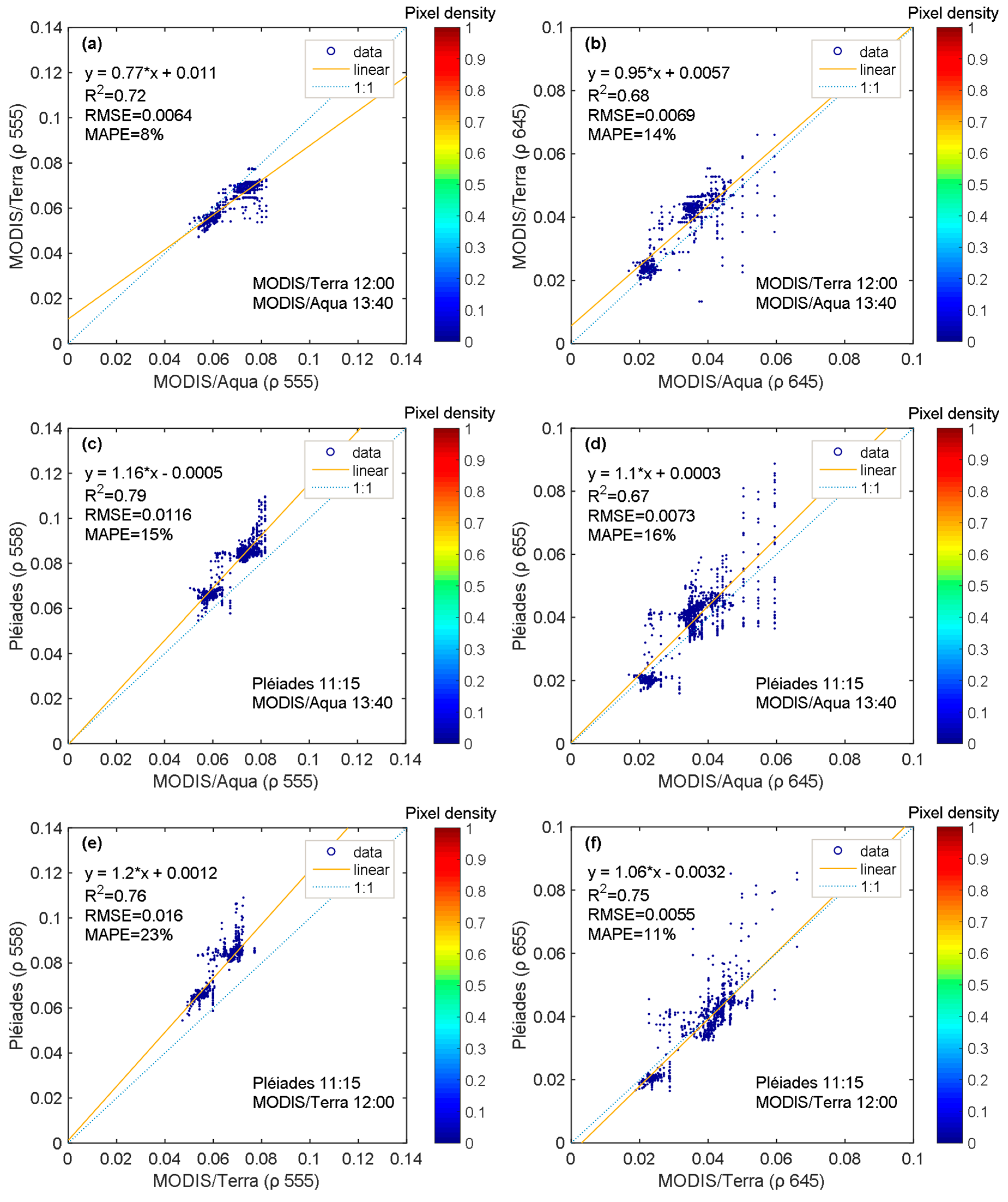
2.3.2. Validation of Atmospheric Correction
2.3.3. Downscaling of Pléiades Spatial Resolution
2.3.4. Accuracy Assessment
3. Results
3.1. Validation of Pléiades-Retrieved Water Reflectances
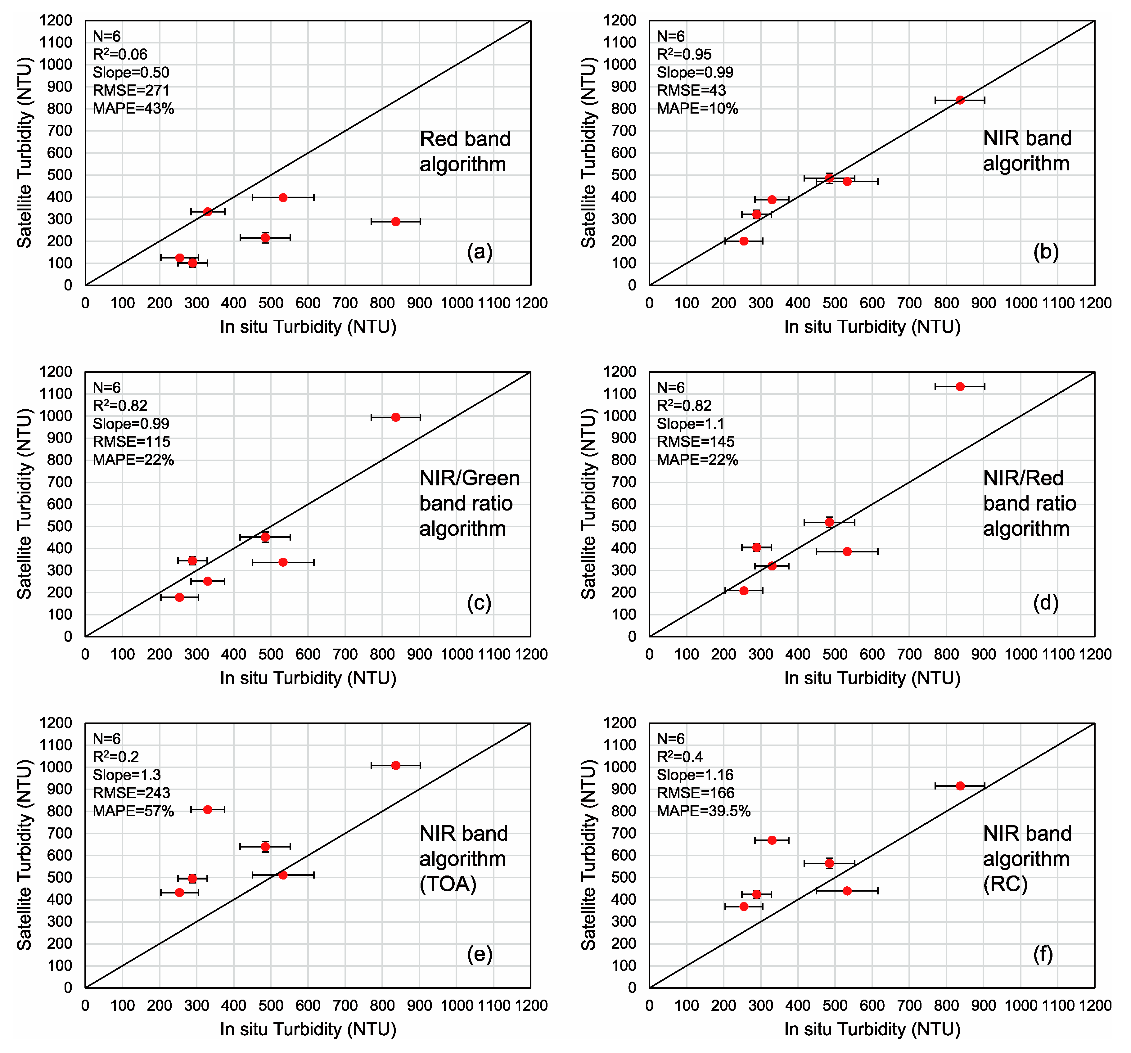
3.2. Validation of Pléiades-Retrieved Water Turbidity
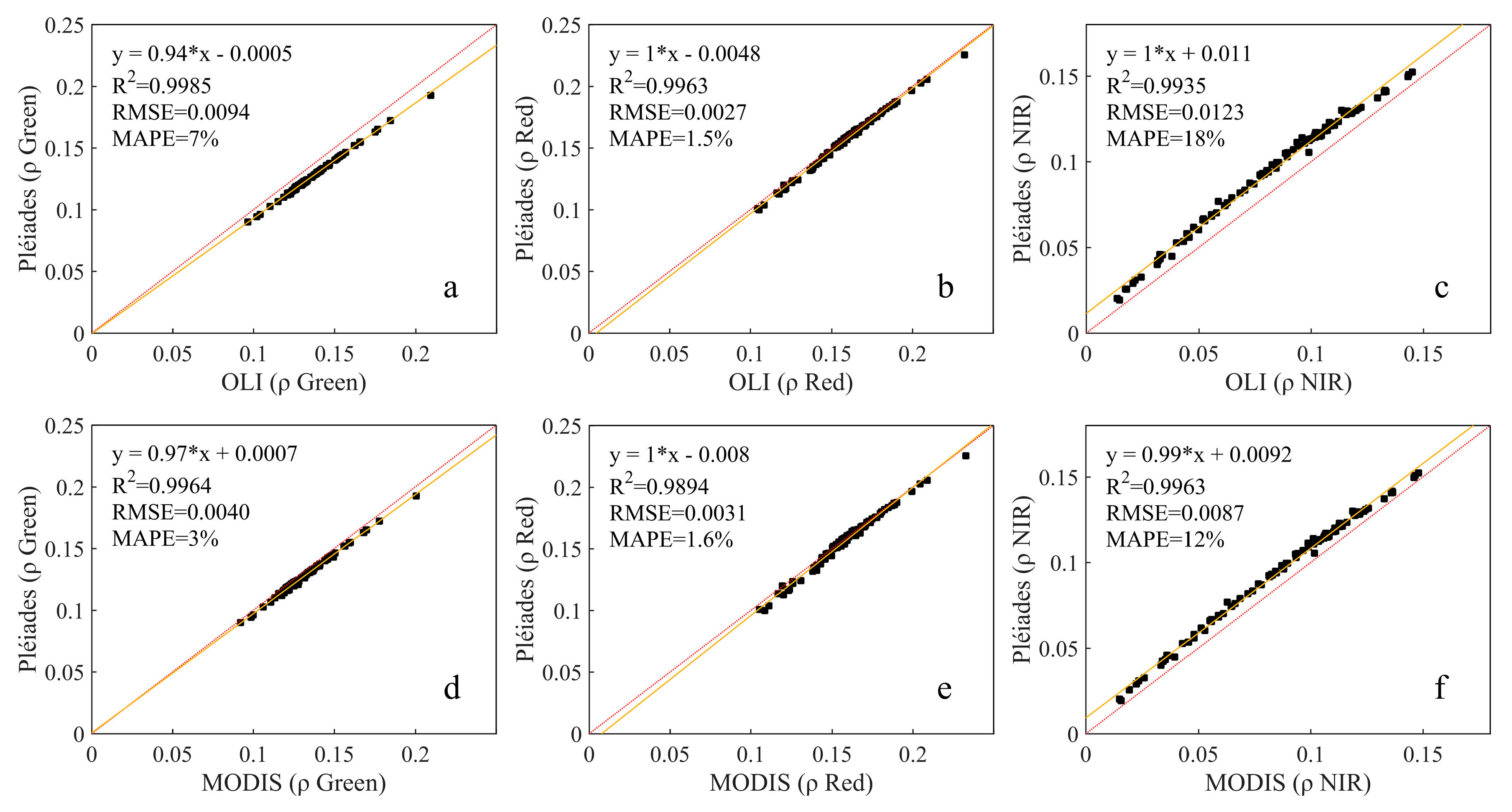
3.3. Impact of Pléiades Band Designations on Water Reflectance and Turbidity Retrievals
3.3.1. Sensor-to-Sensor Band Differences Based on the Relative Spectral Responses
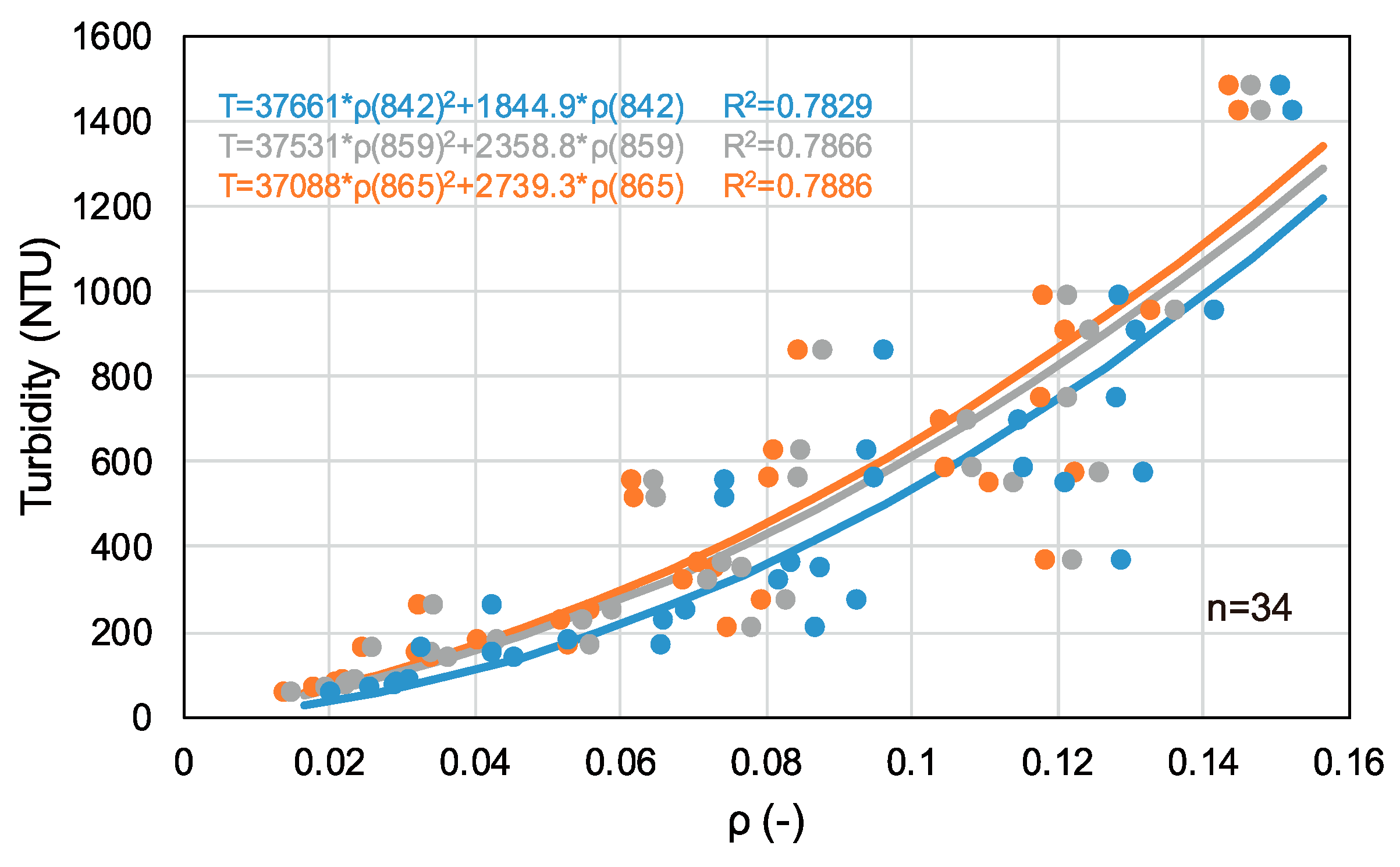
3.3.2. In Situ Water Reflectance and Turbidity Algorithms for Pléiades, OLI and MODIS
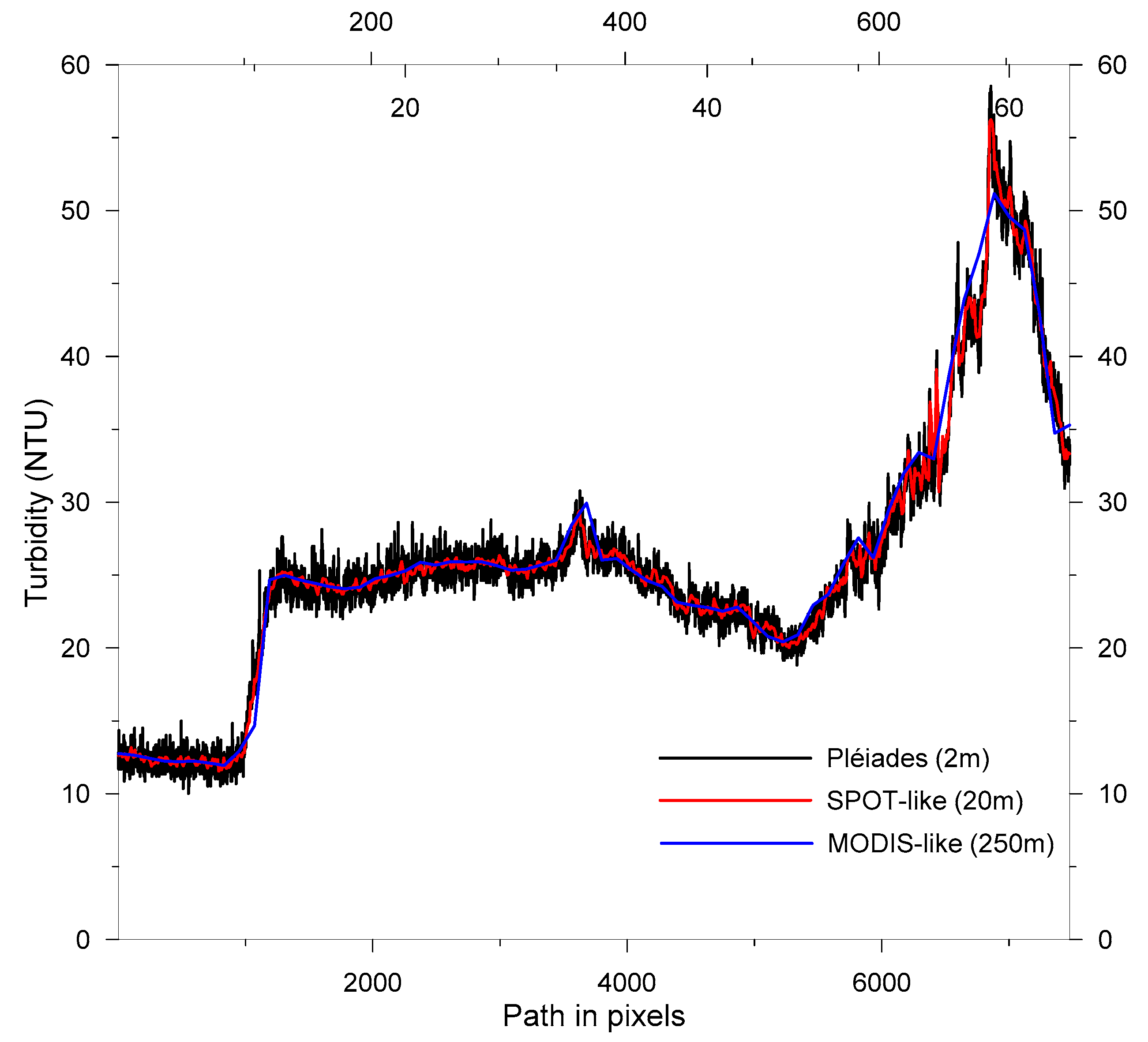
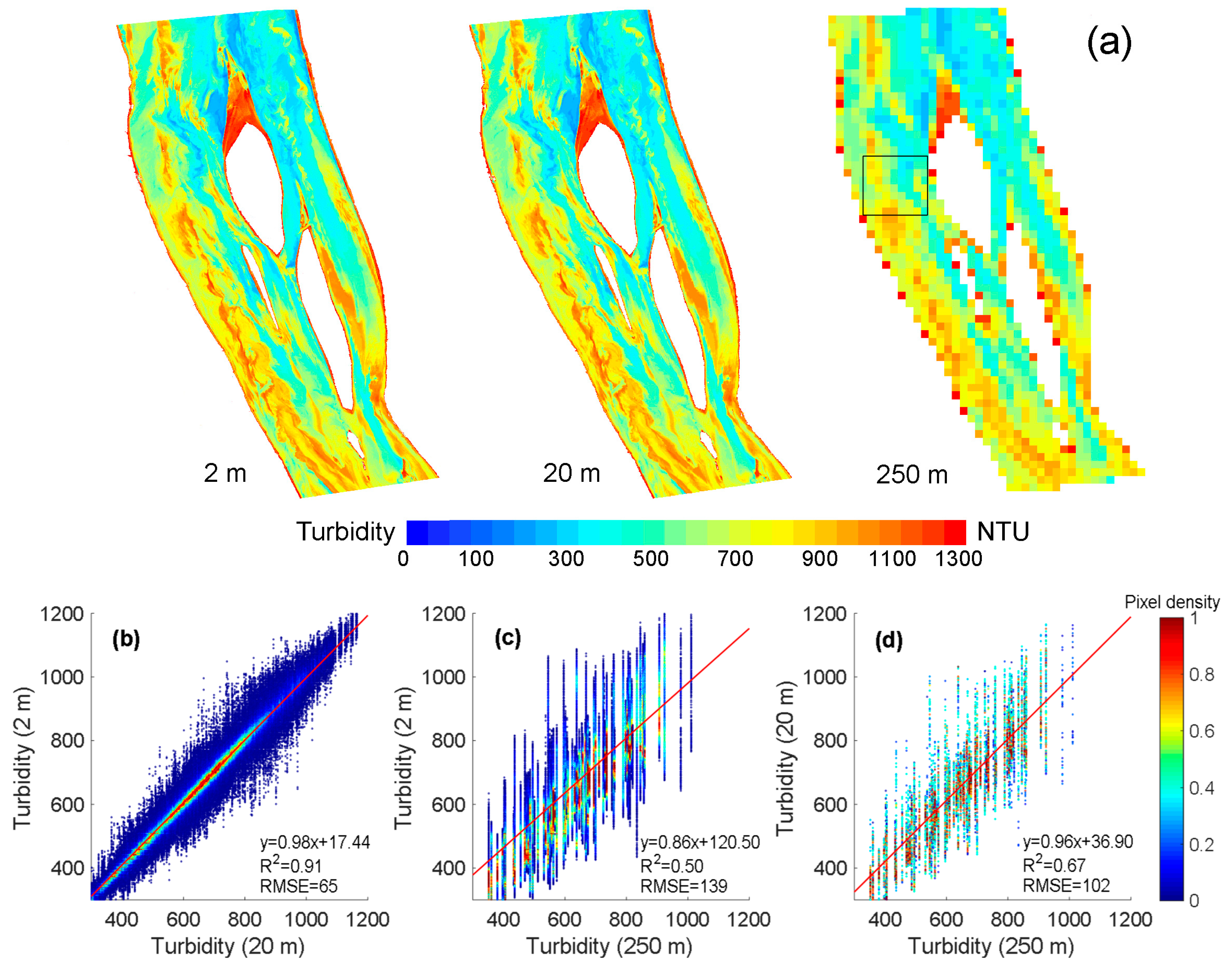
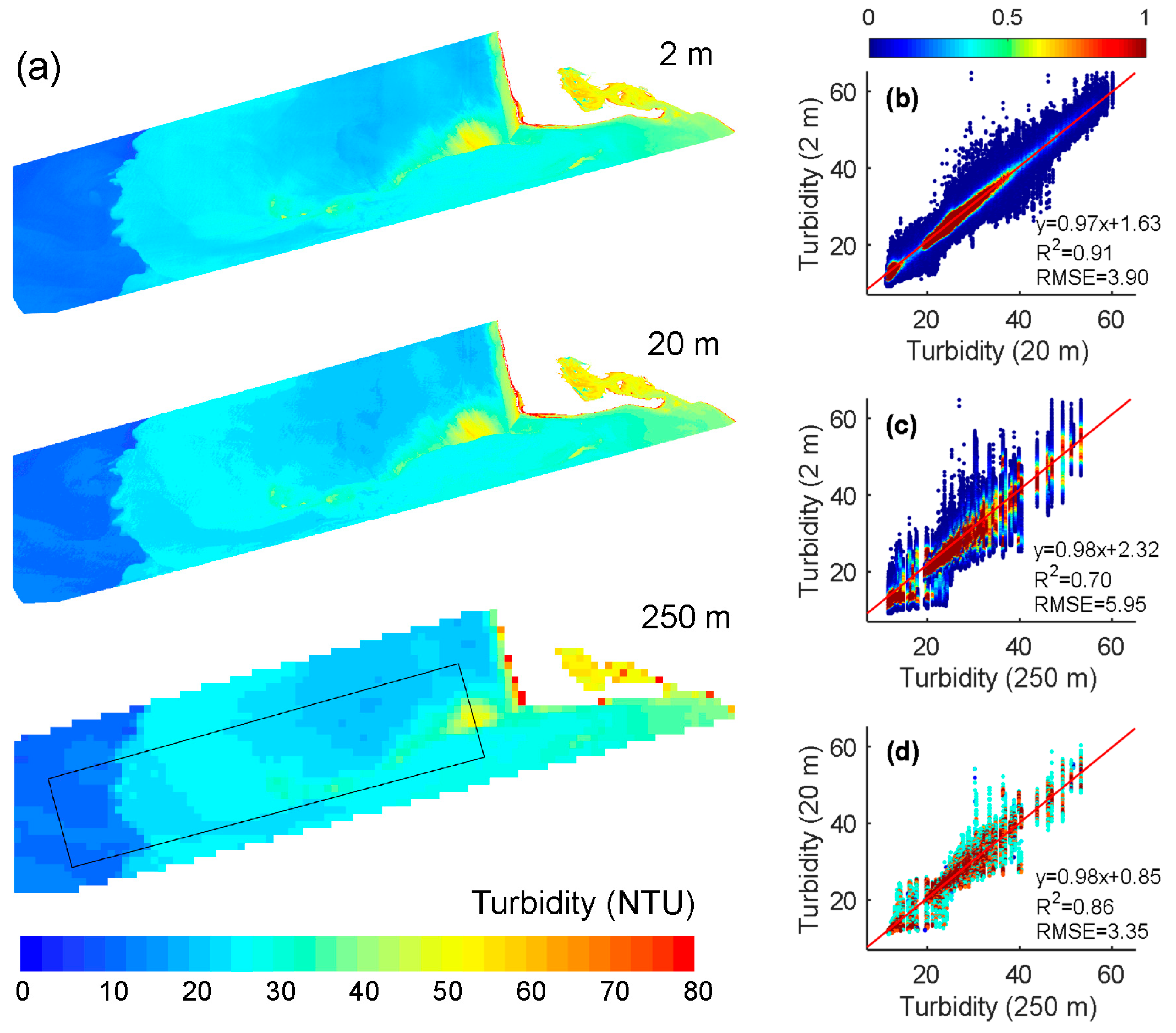
3.4. Impact of Satellite Data Spatial Resolution on Turbidity Retrieval
4. Discussion
4.1. About Validation
4.2. Advantages of Metre-Scale Pléiades Data in Monitoring Water Quality Parameters
4.3. Dataset and Methodology Limitations
5. Conclusions
Author Contributions
Funding
Acknowledgments
Conflicts of Interest
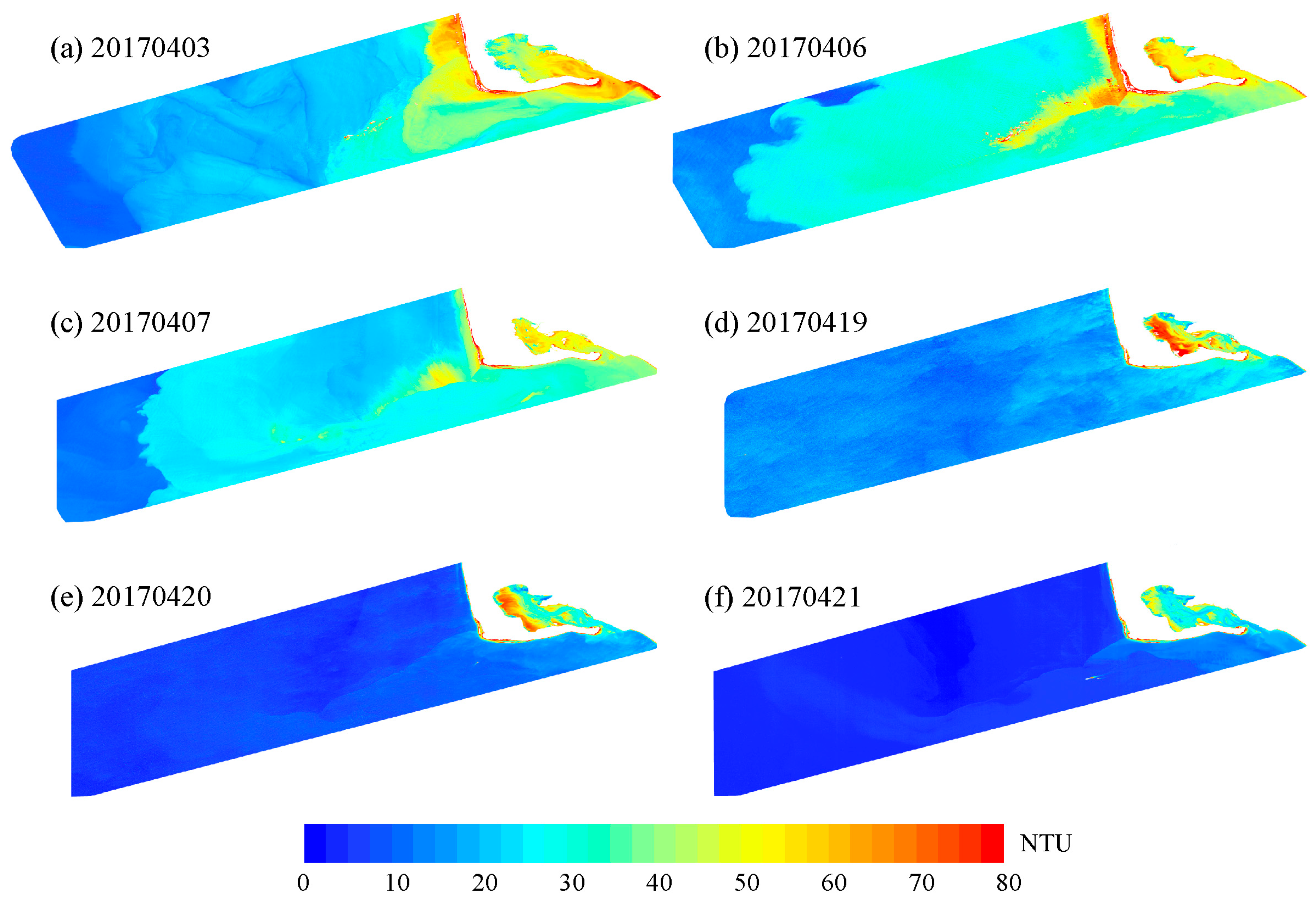
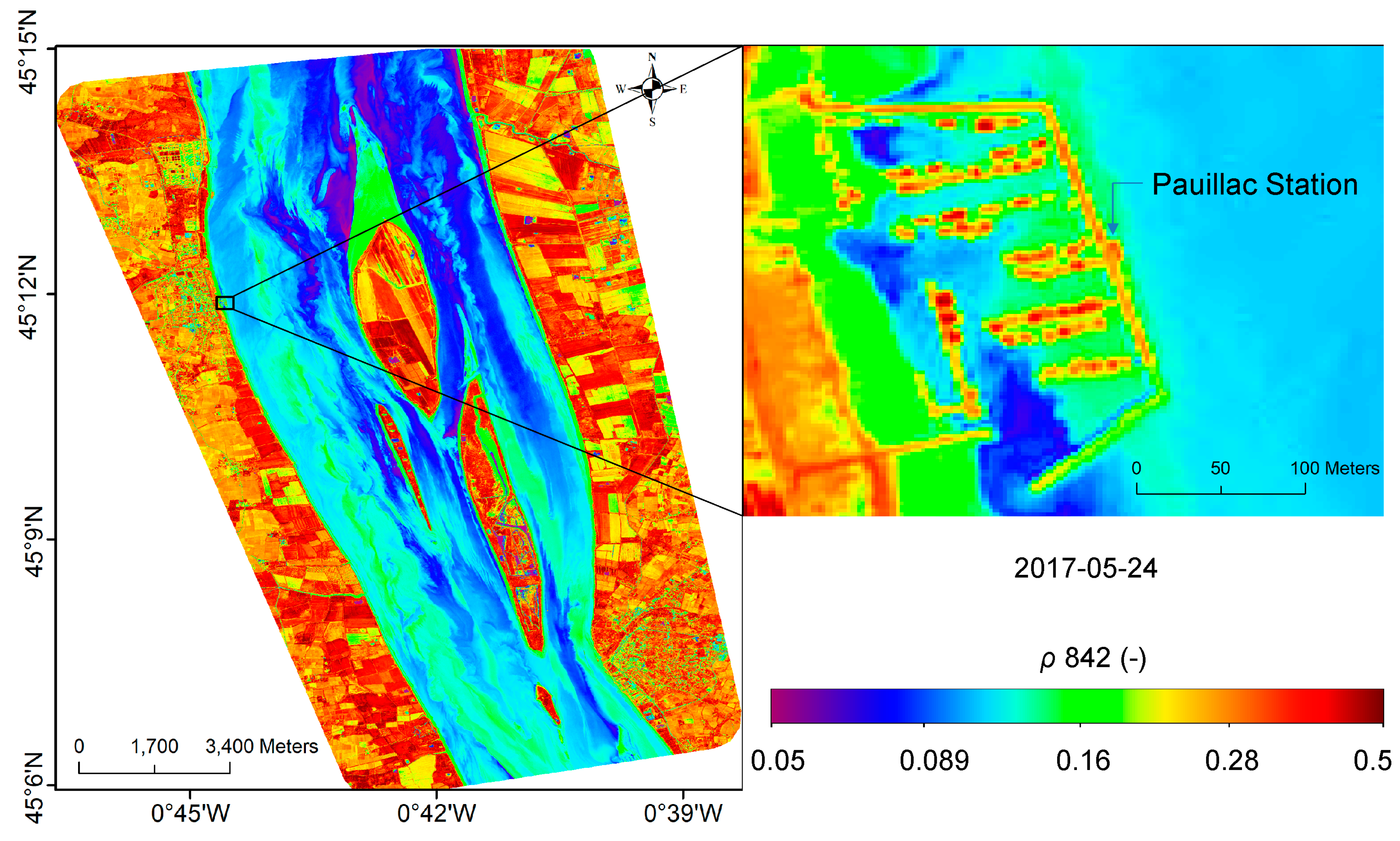
Appendix A. Water Turbidity Mapping

References
- Barnes, B.B.; Hu, C.; Kovach, C.; Silverstein, R.N. Sediment plumes induced by the Port of Miami dredging: Analysis and interpretation using Landsat and MODIS data. Remote Sens. Environ. 2015, 170, 328–339. [Google Scholar] [CrossRef]
- Jay, S.; Guillaume, M. A novel maximum likelihood based method for mapping depth and water quality from hyperspectral remote-sensing data. Remote Sens. Environ. 2014, 147, 121–132. [Google Scholar] [CrossRef]
- Olmanson, L.G.; Brezonik, P.L.; Bauer, M.E. Airborne hyperspectral remote sensing to assess spatial distribution of water quality characteristics in large rivers: The Mississippi river and its tributaries in minnesota. Remote Sens. Environ. 2013, 130, 254–265. [Google Scholar] [CrossRef]
- Doxaran, D.; Devred, E.; Babin, M. A 50% increase in the mass of terrestrial particles delivered by the Mackenzie River into the Beaufort Sea (Canadian Arctic Ocean) over the last 10 years. Biogeosciences 2015, 12, 3551–3565. [Google Scholar] [CrossRef] [Green Version]
- Ozbay, G.; Fan, C.; Yang, Z. Relationship between land use and water quality and its assessment using hyperspectral remote sensing in mid-atlantic estuaries. In Water Quality; IntechOpen: Rijeka, Croatia, 2017. [Google Scholar]
- Ritchie, J.C.; Cooper, C.M. Remote sensing techniques for determining water quality: Applications to TMDLs. In Proceedings of the TMDL Science Issues Conference, Water Environment Federation, Alexandria, VA, USA, 4–7 March 2001; pp. 367–374. [Google Scholar]
- Shang, S.; Lee, Z.; Shi, L.; Lin, G.; Wei, G.; Li, X. Changes in water clarity of the Bohai Sea: Observations from MODIS. Remote Sens. Environ. 2016, 186, 22–31. [Google Scholar] [CrossRef] [Green Version]
- Giardino, C.; Bresciani, M.; Cazzaniga, I.; Schenk, K.; Rieger, P.; Braga, F.; Matta, E.; Brando, V. Evaluation of multi-resolution satellite sensors for assessing water quality and bottom depth of Lake Garda. Sensors 2014, 14, 24116–24131. [Google Scholar] [CrossRef] [Green Version]
- Vanhellemont, Q.; Neukermans, G.; Ruddick, K. Synergy between polar-orbiting and geostationary sensors: Remote sensing of the ocean at high spatial and high temporal resolution. Remote Sens. Environ. 2014, 146, 49–62. [Google Scholar] [CrossRef] [Green Version]
- Vanhellemont, Q. Automated water surface temperature retrieval from Landsat 8/TIRS. Remote Sens. Environ. 2020, 237, 111518. [Google Scholar] [CrossRef]
- Vanhellemont, Q.; Ruddick, K. Turbid wakes associated with offshore wind turbines observed with Landsat 8. Remote Sens. Environ. 2014, 145, 105–115. [Google Scholar] [CrossRef] [Green Version]
- Qiu, Z.; Xiao, C.; Perrie, W.; Sun, D.; Wang, S.; Shen, H.; Yang, D.; He, Y. Using Landsat 8 data to estimate suspended particulate matter in the Yellow River estuary. J. Geophys. Res. Oceans 2017, 122, 276–290. [Google Scholar] [CrossRef]
- Constantin, S.; Doxaran, D.; Constantinescu, Ș. Estimation of water turbidity and analysis of its spatio-temporal variability in the Danube River plume (Black Sea) using MODIS satellite data. Cont. Shelf Res. 2016, 112, 14–30. [Google Scholar] [CrossRef]
- Constantin, S.; Constantinescu, Ș.; Doxaran, D. Long-term analysis of turbidity patterns in Danube Delta coastal area based on MODIS satellite data. J. Mar. Syst. 2017, 170, 10–21. [Google Scholar] [CrossRef]
- Zhang, Y.; Shi, K.; Zhou, Y.; Liu, X.; Qin, B. Monitoring the river plume induced by heavy rainfall events in large, shallow, Lake Taihu using MODIS 250 m imagery. Remote Sens. Environ. 2016, 173, 109–121. [Google Scholar] [CrossRef]
- Doxaran, D.; Froidefond, J.-M.; Lavender, S.; Castaing, P. Spectral signature of highly turbid waters: Application with SPOT data to quantify suspended particulate matter concentrations. Remote Sens. Environ. 2002, 81, 149–161. [Google Scholar] [CrossRef]
- Doxaran, D.; Castaing, P.; Lavender, S. Monitoring the maximum turbidity zone and detecting fine-scale turbidity features in the Gironde estuary using high spatial resolution satellite sensor (SPOT HRV, Landsat ETM+) data. Int. J. Remote Sens. 2006, 27, 2303–2321. [Google Scholar] [CrossRef]
- Gernez, P.; Lafon, V.; Lerouxel, A.; Curti, C.; Lubac, B.; Cerisier, S.; Barillé, L. Toward Sentinel-2 high resolution remote sensing of suspended particulate matter in very turbid waters: SPOT4 (Take5) Experiment in the Loire and Gironde Estuaries. Remote Sens. 2015, 7, 9507–9528. [Google Scholar] [CrossRef] [Green Version]
- Novoa, S.; Doxaran, D.; Ody, A.; Vanhellemont, Q.; Lafon, V.; Lubac, B.; Gernez, P. Atmospheric corrections and multi-conditional algorithm for multi-sensor remote sensing of suspended particulate matter in low-to-high turbidity levels coastal waters. Remote Sens. 2017, 9, 61. [Google Scholar] [CrossRef] [Green Version]
- Doxaran, D.; Froidefond, J.-M.; Castaing, P.; Babin, M. Dynamics of the turbidity maximum zone in a macrotidal estuary (the Gironde, France): Observations from field and MODIS satellite data. Estuar. Coast. Shelf Sci. 2009, 81, 321–332. [Google Scholar] [CrossRef]
- Constantin, S.; Doxaran, D.; Derkacheva, A.; Novoa, S.; Lavigne, H. Multi-temporal dynamics of suspended particulate matter in a macro-tidal river Plume (the Gironde) as observed by satellite data. Estuar. Coast. Shelf Sci. 2018, 202, 172–184. [Google Scholar] [CrossRef]
- Li, J.; Chen, X.; Tian, L.; Huang, J.; Feng, L. Improved capabilities of the Chinese high-resolution remote sensing satellite GF-1 for monitoring suspended particulate matter (SPM) in inland waters: Radiometric and spatial considerations. ISPRS J. Photogramm. Remote Sens. 2015, 106, 145–156. [Google Scholar] [CrossRef]
- Shang, P.; Shen, F. Atmospheric correction of satellite GF-1/WFV imagery and quantitative estimation of suspended particulate matter in the Yangtze estuary. Sensors 2016, 16, 1997. [Google Scholar] [CrossRef] [PubMed] [Green Version]
- Liu, H.; Li, Q.; Shi, T.; Hu, S.; Wu, G.; Zhou, Q. Application of sentinel 2 MSI images to retrieve suspended particulate matter concentrations in Poyang Lake. Remote Sens. 2017, 9, 761. [Google Scholar] [CrossRef] [Green Version]
- Pahlevan, N.; Sarkar, S.; Franz, B.; Balasubramanian, S.; He, J. Sentinel-2 Multispectral Instrument (MSI) data processing for aquatic science applications: Demonstrations and validations. Remote Sens. Environ. 2017, 201, 47–56. [Google Scholar] [CrossRef]
- Caballero, I.; Stumpf, R.P.; Meredith, A. Preliminary Assessment of Turbidity and Chlorophyll Impact on Bathymetry Derived from Sentinel-2A and Sentinel-3A Satellites in South Florida. Remote Sens. 2019, 11, 645. [Google Scholar] [CrossRef] [Green Version]
- Sawaya, K.E.; Olmanson, L.G.; Heinert, N.J.; Brezonik, P.L.; Bauer, M.E. Extending satellite remote sensing to local scales: Land and water resource monitoring using high-resolution imagery. Remote Sens. Environ. 2003, 88, 144–156. [Google Scholar] [CrossRef]
- Ekercin, S. Water quality retrievals from high resolution IKONOS multispectral imagery: A case study in Istanbul, Turkey. Water Air Soil Pollut. 2007, 183, 239–251. [Google Scholar] [CrossRef]
- Liu, J.; Zhang, Y.; Yuan, D.; Song, X. Empirical estimation of total nitrogen and total phosphorus concentration of urban water bodies in China using high resolution IKONOS multispectral imagery. Water 2015, 7, 6551–6573. [Google Scholar] [CrossRef] [Green Version]
- Dorji, P.; Fearns, P. Impact of the spatial resolution of satellite remote sensing sensors in the quantification of total suspended sediment concentration: A case study in turbid waters of Northern Western Australia. PLoS ONE 2017, 12, e0175042. [Google Scholar] [CrossRef]
- Fichot, C.G.; Downing, B.D.; Bergamaschi, B.A.; Windham-Myers, L.; Marvin-DiPasquale, M.; Thompson, D.R.; Gierach, M.M. High-resolution remote sensing of water quality in the San Francisco Bay–Delta Estuary. Environ. Sci. Technol. 2016, 50, 573–583. [Google Scholar] [CrossRef]
- ASTRIUM. PLEIADES Imagery User Guide; An EADS Company, 2012. Available online: https://www.cscrs.itu.edu.tr/assets/downloads/PleiadesUserGuide.pdf (accessed on 3 March 2020).
- Vanhellemont, Q.; Ruddick, K. Atmospheric correction of metre-scale optical satellite data for inland and coastal water applications. Remote Sens. Environ. 2018, 216, 586–597. [Google Scholar] [CrossRef]
- Vanhellemont, Q. Daily metre-scale mapping of water turbidity using CubeSat imagery. Opt. Express 2019, 27, A1372–A1399. [Google Scholar] [CrossRef] [PubMed]
- Vermote, E.; Tanré, D.; Deuzé, J.; Herman, M.; Morcrette, J.; Kotchenova, S. Second Simulation of a Satellite Signal in the Solar Spectrum-Vector (6SV). 6S User Guide Version. 2006, Volume 3, pp. 1–55. Available online: http://6s.ltdri.org/files/tutorial/6S_Manual_Part_1.pdf (accessed on 3 March 2020).
- Kotchenova, S.Y.; Vermote, E.F.; Matarrese, R.; Klemm, F.J. Validation of a vector version of the 6S radiative transfer code for atmospheric correction of satellite data. Part I: Path radiance. Appl. Opt. 2006, 45, 6762–6774. [Google Scholar] [CrossRef] [Green Version]
- Feldman, G.C.; McClain, C.R. l2gen, Ocean Color SeaDAS; NASA Goddard Space Flight Center: Greenbelt, MD, USA, 2010. Available online: https://oceancolor.gsfc.nasa.gov/docs/format/l2oc_modis/ (accessed on 3 March 2020).
- Wang, M.; Wei, S. The NIR-SWIR combined atmospheric correction approach for MODIS ocean color data processing. Opt. Express 2007, 15, 15722–15733. [Google Scholar] [CrossRef] [PubMed] [Green Version]
- Vanhellemont, Q.; Ruddick, K. Advantages of high quality SWIR bands for ocean colour processing: Examples from Landsat-8. Remote Sens. Environ. 2015, 161, 89–106. [Google Scholar] [CrossRef] [Green Version]
- Etcheber, H.; Schmidt, S.; Sottolichio, A.; Maneux, E.; Chabaux, G.; Escalier, J.M.; Wennekes, H.; Derriennic, H.; Schmeltz, M.; Quéméner, L.; et al. Monitoring water quality in estuarine environments: Lessons from the MAGEST monitoring program in the Gironde fluvial-estuarine system. Hydrol. Earth Syst. Sci. 2011, 15, 831–840. [Google Scholar] [CrossRef] [Green Version]
- Schmidt, S.; Etcheber, H.; Sottolichio, A.; Castaing, P. Le reseau MAGEST: Bilan de 10 ans de suivi haute-fréquence de la qualité des eaux de l’estuaire de la Gironde. Mesures Haute Résolution Dans L’environnement Marin Côtier; Schmitt, F.G., Lefevre, A., Eds.; Presses du CNRS, 2016; pp. 51–60. Available online: http://www.magest.u-bordeaux1.fr/files/docs/PublicationHFMAREL2014-SchmidtS.pdf (accessed on 3 March 2020).
- Knaeps, E.; Ruddick, K.G.; Doxaran, D.; Dogliotti, A.I.; Nechad, B.; Raymaekers, D.; Sterckx, S. A SWIR based algorithm to retrieve total suspended matter in extremely turbid waters. Remote Sens. Environ. 2015, 168, 66–79. [Google Scholar] [CrossRef] [Green Version]
- Knaeps, E.; Doxaran, D.; Dogliotti, A.; Nechad, B.; Ruddick, K.; Raymaekers, D.; Sterckx, S. The SeaSWIR dataset. Earth Syst. Sci. Data 2018, 10, 1439–1449. [Google Scholar] [CrossRef] [Green Version]
- Luo, Y.; Doxaran, D.; Ruddick, K.; Shen, F.; Gentili, B.; Yan, L.; Huang, H. Saturation of water reflectance in extremely turbid media based on field measurements, satellite data and bio-optical modelling. Opt. Express 2018, 26, 10435–10451. [Google Scholar] [CrossRef] [Green Version]
- Nechad, B.; Ruddick, K.; Park, Y. Calibration and validation of a generic multisensor algorithm for mapping of total suspended matter in turbid waters. Remote Sens. Environ. 2010, 114, 854–866. [Google Scholar] [CrossRef]
- Vanhellemont, Q. Adaptation of the dark spectrum fitting atmospheric correction for aquatic applications of the Landsat and Sentinel-2 archives. Remote Sens. Environ. 2019, 225, 175–192. [Google Scholar] [CrossRef]


| Characters | Pléiades | SPOT-4 | OLI | MODIS |
|---|---|---|---|---|
| Blue | 450–520 nm | / | 450–515 nm | 459–479 nm |
| Green | 520–600 nm | 500–590 nm | 525–600 nm | 545–565 nm |
| Red | 630–690 nm | 610–680 nm | 630–680 nm | 620–670 nm |
| NIR | 760–900 nm | 780–890 nm | 845–885 nm | 841–876 nm |
| Spatial resolution | 2 m | 20 m | 30 m | 500/250 m |
| Revisit time | 1–3 days | 1–3 days | 16 days | Daily |
| Test Sites | Image Date | Image Time | Time of High Tide | Tidal Range (m) | Satellite/Sensor |
|---|---|---|---|---|---|
| Test site 1 | 03/05/2017 | 11:15 | 10:57 | 3.7 | Pléiades |
| Test site 1 | 24/05/2017 | 11:04 | 16:00 | 5.0 | Pléiades |
| Test site 1 | 01/06/2017 | 10:52 | 10:24 | 3.6 | Pléiades |
| Test site 1 | 10/06/2017 | 11:23 | 05:22 | 4.6 | Pléiades |
| Test site 1 | 14/06/2017 | 10:52 | 07:38 | 3.9 | Pléiades |
| Test site 1 | 19/09/2018 | 10:50 | 13:22 | 2.5 | Pléiades |
| Test site 2 | 03/04/2017 | 10:56 | 08:48 | 3.1 | Pléiades |
| Test site 2 | 06/04/2017 | 11:22 | 13:00 | 2.7 | Pléiades |
| Test site 2 | 07/04/2017 | 11:15 | 13:57 | 3.0 | Pléiades |
| Test site 2 | 19/04/2017 | 11:22 | 09:05 | 1.8 | Pléiades |
| Test site 2 | 20/04/2017 | 11:15 | 11:01 | 1.7 | Pléiades |
| Test site 2 | 21/04/2017 | 11:08 | 12:12 | 1.9 | Pléiades |
| Test site 2 | 07/04/2017 | 10:53 | 13:57 | 3.0 | Landsat8/OLI |
| Test site 2 | 07/04/2017 | 12:00 | 13:57 | 3.0 | Terra/MODIS |
| Test site 2 | 07/04/2017 | 13:40 | 13:57 | 3.0 | Aqua/MODIS |
| Sensor | OLI to Pléiades | MODIS to Pléiades | ||||
|---|---|---|---|---|---|---|
| Band | Relationships | RMSE | MAPE | Relationships | RMSE | MAPE |
| Green | y = 0.94*x − 0.0005 | 0.0094 | 7% | y = 0.97*x + 0.0007 | 0.0040 | 3% |
| Red | y = 1.00*x − 0.0048 | 0.0027 | 1.5% | y = 1.00*x − 0.0080 | 0.0031 | 1.6% |
| NIR | y = 1.00*x + 0.0110 | 0.0123 | 18% | y = 0.99*x + 0.0092 | 0.0087 | 12% |
| Test Site 1 | MAPE (%) | RMSE (NTU) |
|---|---|---|
| Pléiades | 16.6% | 107 |
| OLI | 15.0% | 104 |
| MODIS | 15.4% | 105 |
© 2020 by the authors. Licensee MDPI, Basel, Switzerland. This article is an open access article distributed under the terms and conditions of the Creative Commons Attribution (CC BY) license (http://creativecommons.org/licenses/by/4.0/).
Share and Cite
Luo, Y.; Doxaran, D.; Vanhellemont, Q. Retrieval and Validation of Water Turbidity at Metre-Scale Using Pléiades Satellite Data: A Case Study in the Gironde Estuary. Remote Sens. 2020, 12, 946. https://doi.org/10.3390/rs12060946
Luo Y, Doxaran D, Vanhellemont Q. Retrieval and Validation of Water Turbidity at Metre-Scale Using Pléiades Satellite Data: A Case Study in the Gironde Estuary. Remote Sensing. 2020; 12(6):946. https://doi.org/10.3390/rs12060946
Chicago/Turabian StyleLuo, Yafei, David Doxaran, and Quinten Vanhellemont. 2020. "Retrieval and Validation of Water Turbidity at Metre-Scale Using Pléiades Satellite Data: A Case Study in the Gironde Estuary" Remote Sensing 12, no. 6: 946. https://doi.org/10.3390/rs12060946