Abstract
Improving the spatial resolution of microwave satellite soil moisture (SM) products is important for various applications. Most of the downscaling methods that fuse optical/thermal and microwave data rely on remotely sensed land surface temperature (LST) or LST-derived SM indexes (SMIs). However, these methods suffer from the problems of “cloud contamination”, “decomposing uncertainty”, and “decoupling effect”. This study presents a new downscaling method, referred to as DSCALE_mod16, without using LST and LST-derived SMIs. This model combines MODIS ET products and a gridded meteorological data set to obtain Land surface Evaporative Efficiency (LEE) as the main downscaling factor. A cosine-square form of downscaling function was adopted to represent the quantitative relationship between LEE and SM. Taking the central part of the United States as the case study area, we downscaled SMAP (Soil Moisture Active and Passive) SM products with an original resolution of 36km to a resolution of 500m. The study period spans more than three years from 2015 to 2018. In situ SM measurements from three sparse networks and three core validation sites (CVS) were used to evaluate the downscaling model. The evaluation results indicate that the downscaled SM values maintain the spatial dynamic range of original SM data while providing more spatial details. Moreover, the moisture mass is conserved during the downscaling process. The downscaled SM values have a good agreement with in situ SM measurements. The unbiased root-mean-square errors (ubRMSEs) of downscaled SM values is 0.035 m3/m3 at Fort Cobb, 0.026 m3/m3 at Little Washita, and 0.055 m3/m3 at South Fork, which are comparable to ubRMSEs of original SM estimates at these three CVS.
1. Introduction
Soil moisture (SM) is usually defined as the water contained in the unsaturated soil zone. It can be expressed in a relative quantity (i.e., g/m3, m3/m3, and %) or an absolute quantity (i.e., mm for water depth and kg for mass). The SM in m3/m3 is known as volumetric soil moisture, which is defined as the volume of water in the soil divided by the volume of soil containing the water. SM is the main water resource for crop and natural vegetation growth, which in turn influences on food security and ecological environment. It also plays a significant role in land surface water and energy cycle through partitioning available energy into sensible heat flux and latent heat flux as well as partitioning precipitation into penetration and runoff. On a larger scale, it influences various processes and feedback loops within the Earth system [1]. Consequently, SM is a key parameter in a wide range of applications such as agricultural production [2], drought monitoring and prediction [3,4,5], water resource management [6], weather prediction [7], and climate change [8]. The Global Climate Observing System (GCOS) also recognize the SM as one of the Essential Climate Variables [9,10].
To obtain SM measurements, various techniques have been developed. These include ground measurements, remote sensing measurements, atmospheric-terrestrial water-balance (ATWB) estimates, and land surface model (LSM) based estimates [1]. SM are affected by soil texture, structure, topographic features, land cover patterns, and meteorological forcing conditions at various scales, exhibiting a high spatial heterogeneity [11]. ATWB estimates are difficult to used for trend detection and their spatial resolution is very coarse (300–1000 km). LSM-based estimates are dependent on the quality of forcing data, such as precipitation and radiation. The ground measurements may come from gravimetric methods, time domain reflectometry, and cosmic-ray neutron probes [12]. The point measurements from these ground-based methods are often spatially very sparse and are unable to capture the complete spatial distribution. Satellite remote sensing has become a useful way for obtaining spatially distributed SM measurements from regional to global scales at a regular time interval, although it only retrieves surface soil moisture up to a few centimeters deep at most [10].
The remote sensing measurements of SM can be derived by various retrieving methods that almost utilize the whole spectrum range from visible to microwave bands [10]. The retrieval methods based on visible, near infrared, and thermal infrared bands have a longer history and possess the advantages of high spatiotemporal resolution and abundant data sources. Nevertheless, they suffer from the common drawbacks of optical remote sensing, such as, unavailability under cloudy weather conditions and shallow penetration in soil [10,12,13,14,15]. Owing to the longer wavelength and more direct correlation with SM, microwave bands, especially the L-band, are recognized as the optimal selection for obtaining SM estimates [10,12,13,14,15]. SMOS (Soil Moisture and Ocean Salinity) [16] and SMAP (Soil Moisture Active Passive) [17] are two operational L-band microwave satellite missions for remote sensing of soil moisture. The SMOS, launched on 2 November 2009, provides multi-angular (0°–65°) and full-polarimetric observations with a spatial resolution of about 35–50 km [18]. The SMAP, launched on 31 January 2015, carries two payloads: a real aperture radiometer and a Synthetic Aperture Radar (SAR), providing a single angle (40°) and full-polarimetric observations at spatial resolutions of about 36 km and 3 km, respectively. SMAP mission is designed to provide soil moisture products at low (about 40 km), high (about 3 km) and intermediate (about 10 km) spatial resolutions using observations from the radiometer, SAR, and a combination of the two, respectively. Unfortunately, the SAR sensor experienced a fatal anomaly and no longer transmitted data since 7 July 2015 [19]. In this context, spatial downscaling of microwave soil moisture to higher resolutions, such as one kilometer or even hundreds of meters, is becoming more challenging. It entails the development of new SM downscaling methods in order to support hydrological and agricultural application on a regional or local scale [10,12].
In recognition of the pressing need for downscaling microwave remotely sensed SM data, various methods have been proposed. As summarized in a comprehensive review in [12], the proposed downscaling methods include satellite-based methods, geoinformation-based methods, and model-based methods. Geoinformation-based and model-based methods are either too complicated to implement, dependent upon too many ancillary data, or/and catchment-specific, which clearly limits their applicability. Satellite-based methods have gained popularity among researchers since the abundant and accessible high-resolution remote sensing data have been available. Satellite-based methods can be further divided into active and passive microwave data fusion methods and optical/thermal and microwave fusion methods. The former fusion methods are limited by the availability of matched active and passive microwave data. For example, after the SMAP’s active radar sensor stopped working, some researchers sought to incorporate C-band active microwave data from Sentinel-1 satellite to downscale the SMAP L-band passive microwave data [14,20]. However, this approach faces some technical challenges due to data latency, spatial coverage, revisit frequency, penetration depth, and retrieval performance [21]. Owing to the abundant data source, relative mature observation technology, and well-defined physics, optical/thermal and microwave fusion methods represent the most promising approach to the SM downscaling problem.
Currently, there are three types of optical/thermal and microwave fusion methods: statistical regression, relative ratio, and physical model for simplification. The statistical regression method either uses empirical polynomial fitting [22] or machine learning algorithms [23] to construct a statistical relationship between soil moisture and various land surface parameters, such as, Land Surface Temperature (LST), Normalized Difference Vegetation Index (NDVI), Albedo [22], or microwave brightness temperature [24]. The relative ratio methods assume that high-resolution soil moisture is proportional to the ratio of coarse-resolution soil moisture to a high-resolution soil wetness index [25]. The soil wetness index is actually calculated from the feature space of LST and Fractional Vegetation Coverage or vegetation index (LST/FVC space) [26,27]. Vegetation Temperature Condition Index (VTCI) or Temperature Vegetation Dryness Index (TVDI) have been incorporated to further improve the performance of the relative ratio methods [28,29]. Disaggregation based on Physical and Theoretical scale Change (DISPATCH) is representative of the physical models [30,31]. Its physical basis is the linear, exponential, or cosine expressions of the relationship between SM and soil evaporative efficiency (SEE). SEE is defined as the ratio of actual soil evaporation to the potential one over soil surface. In the DISPATCH model, SEE is calculated as the relative distance of soil temperature to its extreme values at the conditions of maximum water stress and saturated water supply [31]. The soil temperature and its extreme values were determined from the LST/FVC space. The determination of SEE in DISPATCH is very similar to the calculation of VTCI or TVDI, which are all derived from the LST/FVC space. We refer to these variables as the LST-derived soil moisture indices (SMIs). Apparently, the LST and LST-derived SMIs are vital to the optical/thermal and microwave fusion methods for disaggregating microwave satellite SM.
Nevertheless, most downscaling methods based on LST and LST-derived SMIs need to tackle “cloud contamination”, “decomposing uncertainty”, and “decoupling effect” problems. Firstly, LST cannot be retrieved from thermal remote sensing data in cloudy weather condition. The downscaling methods that are based on LST and LST-derived SMIs are not able to operate under all-weather conditions. Secondly, there are greater uncertainties in decomposing remotely sensed LST into soil and vegetation temperature components to calculate the LST-derived SMIs. It is very difficult to accurately determine the dry and wet boundaries of the LST/FVC space [32]. For instance, the DISPATCH algorithm obtains the soil and vegetation temperature end-members from remote sensing image itself [19]. However, it is not always the case that there exist pixels under very dry and wet conditions and can be used as end-members in a study area. For the areas without such extreme pixels, the temperature end-members selected are not true end-members, which brings great uncertainties in downscaling SM. Furthermore, there are diverse models to interpret the LST/FVC space, which complicate the process of decomposing remotely sensed LST. At least three models exist for the interpretation of LST/FVC space in the literature, namely, the triangle model [33,34], the conventional trapezoid model [35], and the two-stage trapezoid model [26]. Thirdly, there exists decoupling effect among SM, LST, and LST-derived SMIs both in very wet and in very dry condition [36]. Such decoupling effect can degrade the performance of LST as a downscaling factor [36]. The above problems have severely hampered the development and extensive application of the downscaling methods that rely on LST and LST-derived SMIs. [12,20].
To address the above “cloud contamination”, “decomposing uncertainty”, and “decoupling effect” problems, this study presents a novel downscaling method for disaggregating microwave satellite SM. Instead of using LST or LST-derived SMIs, our method utilizes Land surface Evaporative Efficiency (LEE) as the main downscaling factor. LEE is defined as the ratio of actual evapotranspiration (ET) to potential ET (PET). MODIS (Moderate Resolution Imaging Spectroradiometer) ET production (MOD16) and gridded meteorological data are the main data sources for determining the LEE. We refer to this new method as DSCALE_mod16 for the presentation convenience. Since the DSCALE_mod16 model does not depend on LST or LST-derived SMIs, the “cloud contamination”, “decomposing uncertainty”, and “decoupling effect” problems can then be circumvented. The DSCALE_mod16 algorithm will be illustrated in detail in Section 2. Section 3 describes the data sets that we used in this study. The evaluation of the DSCALE_mod16 model performance is presented in Section 4. Then, we discuss the DSCALE_mod16 algorithm and relevant application issues in Section 5 and draw some conclusions in Section 6.
2. DSCALE_mod16 Model
2.1. Overview of the Model Components and Structure
Figure 1 shows the structure and data flow of the DSCALE_mod16 model. MODIS ET products (MOD16), original microwave remotely sensed coarser-resolution SM (), and gridded meteorological data are three input data sources for the DSCALE_mod16 model. The MOD16 products were processed with the vegetated module in order to calculate LEE for vegetated areas. As the MOD16 products did not calculate ET for non-vegetated areas, the gridded meteorological data were employed to approximate LEE over barren or sparsely vegetated areas with the barren module. Subsequently, we integrate the LEE estimates from vegetated module and barren module to obtain a spatially continuous higher-resolution LEE (). Finally, higher-resolution SM () measurements are derived through coupling the and a downscaling module. Specific details of the three modules, i.e., Barren module, Vegetated module, and Downscaling module are introduced as follows.
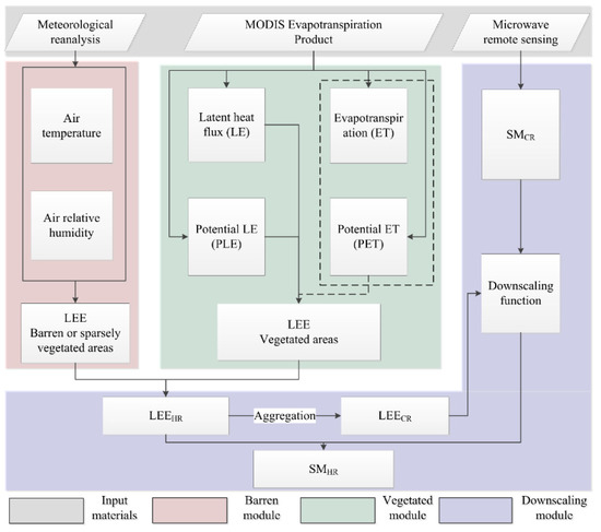
Figure 1.
Component modules and data flow of the DSCALE_mod16 model for disaggregating coarse-resolution soil moisture data. LEE: Land surface evaporative efficiency, SM: soil moisture. The subscripts HR and CR represent high-resolution and coarse-resolution, respectively.
2.2. Vegetated Module
LEE can be expressed as
where LE is actual land surface latent heat flux (W/m2) and PLE is potential LE (W/m2). Since the denominator PLE is defined as the latent heat flux with sufficient water supply and the numerator LE corresponds to actual water supply, their ratio LEE is therefore a powerful indicator of SM variation. As matter of fact, this indicator has been widely used in constructing drought a severity index. For instance, the Evaporative Drought Index (EDI) is expressed as EDI=1−LEE [37]. The Evaporative Stress Index (ESI) is defined as the standardized anomalies in the LEE [38]. The Drought Severity Index (DSI) is defined as the sum of the normalized LEE and the normalized NDVI [39]. Previous studies have suggested that LEE is a valid indicator for characterizing SM anomalies and drought [3,40].
In this study, MODIS ET products (MOD16A2) were used to calculate the LEE. The MODIS ET product is based on the logic of the Penman-Monteith equation that uses remotely sensed vegetation property dynamics derived from MODIS without using remotely sensed LST and LST-derived SMIs [29]. MOD16A2 has a temporal resolution of 8-day which is the highest temporal resolution in current MODIS ET products. We assume that the calculated LEE is relatively stationary during the 8-day interval. It should be noted that the MODIS ET products do not have full spatial coverage owing to the variation in land cover types. Table 1 shows the land cover types where the MOD16A2 derived ET estimates are not available. Alternative approaches are necessary for estimating the LEE over the land cover types where the MODIS derived ET are not available (Table 1). In this study, the LEE over urban built-up, impervious surface, and permanent snow and ice-covered areas was assigned a value of zero, since there is no available water for ET. The LEE over water bodies and permanent wetland was given a value of 1.0, because there is sufficient water for ET. The LEE over barren or sparsely vegetated and unclassified areas was determined using the Barren module, which will be described below. In some rare situation where the soil moisture is nearly saturated, the calculated LE may be greater than PLE. In this case, we simply set the LEE value to 1.0 in order to constrain the LEE to the range of [0, 1.0].

Table 1.
The land cover types where the ET is not produced in MOD16A2 dataset.
2.3. Barren Module
The barren module estimates the LEE based on a complementary hypothesis that surface soil moisture dynamic can be indicated by surface meteorological variables at mid-day conditions [20]. LEE is estimated in Barren module by the following equation:
where represents the wet surface fraction used to divide soil surface into saturated surface and the moist surface [29,41]. RH is the relative humidity; VPD is the saturation vapor pressure deficit; and is a parameter defined as the relative sensitivity to VPD. is set as 1.0 kPa as according to Fisher et al. (2008) [41]. Wet surface fraction can be determined by the following way [29]:
It should be noted that the optimized condition for the complementary relationship hypothesis is in midday when convective conditions induce strong vertical mixing and significant influence of land surface on the atmosphere [41]. Consequently, the RH and VPD should be calculated using midday conditions rather than daily averages for the calculation of LEE:
where is daily maximum air temperature, is the RH at the time of appearing, and represents vapor pressure function with a variable of (in °C).
2.4. Downscaling Module
Through the above vegetated module and barren module, spatial full coverage of LEEHR can be created. The LEEHR was then aggregated into a coarser-resolution LEE (i.e., LEECR) using arithmetic average, the same spatial resolution as the SMCR. Subsequently, many pairs of LEECR and SMCR were utilized to determine the parameter for the following downscaling function [31,42]:
where is volumetric SM (m3/m3); represents a given critical SM value that plays the threshold role for separating between energy-limited and soil moisture-limited ET regimes [1]. Note that the parameter is critical to derive the higher-resolution SM. It has been recognized that the parameter is an effective parameter rather than a pure physical parameter when the above equation was applied with remote sensing data over larger spatiotemporal domain [20]. The parameter can be determined from given coarser-resolution SM () and aggregated coarser-resolution LEE () data pairs. First, we calculated the critical SM value at coarser-resolution () from the following equations:
Subsequently, we determine the critical SM value at higher-resolution () through spatially interpolating the estimated coarse-resolution with the bilinear interpolation method. It utilizes four coarse resolution pixels to determine the output value, in consistent with the interpolation of meteorological data in the MOD16 evapotranspiration product [29]. Finally, the SM at higher spatial resolution () can be obtained by the following equation:
where HR denotes the high spatial resolution. LEEHR is estimated by the above vegetated module and barren module.
3. Study Area and Data Sets
3.1. Study Area
Figure 2 shows our study area in the cylindrical equal area map projection. It locates in the central United States, covering parts of the states of Oklahoma, Arkansas, Kansas, Missouri, and Iowa. As a part of the Great Plains, the landform of the study area is characterized by a broad expanse of flat land. It has semi-arid continental climate, cold in the winter and hot in the summer. The dominant land covers include prairie, steppe, and grassland. There are also croplands in this study area.
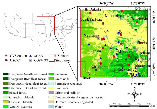
Figure 2.
Spatial distribution of the study area, core validation station (CVS), and three sparse networks (COSMOS, SCAN, USCRN) in situ stations of measuring soil moisture at ground.
3.2. MODIS ET Products
MODIS global ET dataset (MOD16A2) within five tiles of h09v05, h10v04, h10v05, h11v04, and h11v05 during 2015 to 2018 were used in this study. The MOD16A2 has a spatial resolution of 500 m and a temporal resolution of 8 days. There are four main data sets in the MOD16A2 product i.e., ET, PET, LE, and PLE. It should be noted that the ET and PET are the summation of 8-day total ET (kg/m2/8day), whereas the LE and PLE are the average total energy over a unit area for a unit day during the composite 8-day period (J/m2/day). Therefore, two LEEs can be calculated from MOD16A2, respectively, by ET/PET and LE/PLE.
3.3. SMAP Soil Moisture Products
SMAP SM products by L-band passive radiometer were used in this study. Specifically, the level 3 daily composite SM product, SMAP L3 Radiometer Global Daily 36 km EASE-Grid Soil Moisture (SPL3SMP) is the primary variable to be downscaled. Since September 2015, many versions of the SPL3SMP products have been produced. For this study, we used the latest version, Version 6 with Composite Release ID of R16510.
There are SM at A.M. and P.M in each SPL3SMP product. In this study, the SM at A.M. was selected. For the SM at A.M data, a level 2 data point acquired closest to 6:00 A.M. local solar time for a given grid cell will make its way to the final level 3 product; other “late-coming” data points are ignored [15]. All the collected SPL3SMP products were converted to daily SM data at the spatial resolution of 36 km in the WGS_1984_EASE_Grid_Global projection.
3.4. Gridded Meteorological Data
A gridded meteorological dataset GRIDMET [43] was selected because it contains the climate variables RH and Tmax that were required by our barren module. GRIDMET contains daily moderate spatial resolution (nominal ~4 km, 1/24th degree) surface meteorological data, covering the contiguous US since 1979. The GRIDMET has been validated against an extensive network of weather stations. Median correlations for Tmax is estimated to be 0.94–0.95, with a median mean absolute error (MAE) of 1.7–2.3 °C. Humidity has a median correlation value of 0.81 and median MAE of 6–12% [43].
3.5. In Situ Soil Moisture Observation
In situ SM observations based on three sparse networks and three core validation sites (CVS) were used as ground truth to evaluate the downscaling method. Figure 2 shows the locations of all in situ SM measurement sites in our study area. The three sparse networks are Cosmic-ray Soil Moisture Observing System (COSMOS), U.S. Department of Agriculture Soil Climate Analysis Network (SCAN), and U.S. Climate Reference Network (USCRN). There are 59 stations in the sparse networks in total, 12 from the COSMOS, 33 from the SCAN, and 14 from the USCRN. The three CVSs are South Fork in Iowa, Fort Cobb and Little Washita in Oklahoma. All of the in situ SM in sparse networks were obtained from the International Soil Moisture Network (ISMN). All SM data obtained from ISMN are in common volumetric soil moisture unit with quality-control procedures to flag outliers and implausible values [44]. COSMOS measured SM at the depth from top surface to about ten or twenty centimeters. In contrast, SCAN and USCRN networks provide SM at various depths of measurements. The SM observations of SCAN and USCRN at a depth of 0.05m were retained for analysis. The in situ SM observations are hourly data recorded in Coordinated Universal Time (UTC) time. In order to match the remotely sensed SM, the in situ SM observations within the local solar time range from 5:00 A.M. to 7:00 A.M. were averaged to match the SMAP SM at 6:00 A.M. The in situ SM at CVSs were from SMAP/In Situ Core Validation Site Land Surface Parameters Match-Up Data, Version 1 [45]. In this dataset, in situ SM from CVSs have been processed through arithmetic average or weighted average to match SMAP L2 SM products. These in situ SM at CVSs that matched with the SMAP Enhanced L2 Radiometer Half-Orbit 9 km EASE-Grid Soil Moisture (SPL2SMP_E) were adopted in our study. The dataset covers the period from 1 April 2015 to 31 October 2016.
4. Results
4.1. Dynamic Range and Mass Conservation Analysis
In order to evaluate the downscaling method, we firstly compare the downscaled results with their original SM data from the perspective of spatial dynamic range. Figure 3 shows the comparisons over the entire study area, where Figure 3a–c are original SM on July 10, August 11 and October 9 in 2017 and Figure 3d–f are the corresponding downscaled results. The comparisons indicate that the downscaling method can maintain the spatial dynamic range of original SM data. The downscaled SM maps are consistent with their original SM maps in terms of general spatial patterns of SM variation over the whole study area.
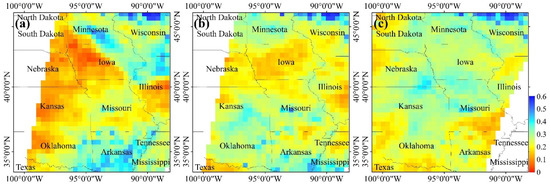
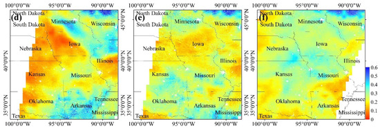
Figure 3.
Comparisons between original and downscaled SM on July 10 (a,d), August 11 (b,e) and October 9 (c,f) in 2017.
Apparently, the downscaled results provide more spatial details of SM variation. Figure 4 shows more detailed comparisons between original SM and downscaled SM on August 11, 2017, where the land cover types were identified by MODIS Land Cover Type Yearly L3 Global 500 m product (MCD12Q1). The first column shows the land cover types and the second column is original SM. The third column illustrates the downscaled SM. It can be observed from the downscaled maps that SM is greater near water or river areas and it decreases with the distance from water areas. The downscaled SM maps provide much more detailed description of SM spatial variation than original SM maps.
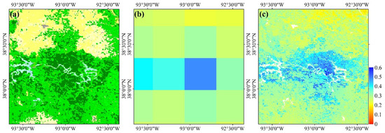
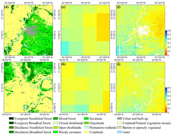
Figure 4.
Comparisons of spatial details between original SM (b,e,g) and downscaled SM (c,f,i) on August 11, 2017 where (a,d,g) are the land cover types.
In addition, we evaluated the downscaled results in terms of mass conservation property. For this evaluation purpose, we aggregated the downscaled SM to the same spatial resolution as their original SM and subtracted the aggregated SM from the original SM data. The difference between the original and aggregated SM data is the indicator of energy conservation. Figure 5a–c shows such differences on the same days as in Figure 3. We can see that the differences are very close to 0 for most of the area. Figure 5d–f are the statistical histograms of the above differences, where μ is the mean and σ is standard deviation of the differences. The mean μ of the differences is −0.04×10⁻² m3/m3, −0.10×10⁻² m3/m3, and −0.19×10⁻² m3/m3 for these three days, which are very close to zero. The standard deviation σ of the differences is 1.47×10⁻² m3/m3, 1.44×10⁻² m3/m3, and 1.27×10⁻² m3/m3, which are also very small. We further analyzed the differences over the entire study period from 2015 to 2018 and results are shown in Figure 6. The mean of the differences varies between -0.004 m3/m3 and 0.004 m3/m3, and the standard deviation of the differences varies between 0 and 0.020 m3/m3. The near-zero mean and tiny standard deviation of the differences indicate that the moisture mass is conserved during the downscaling process. Namely, our downscaling model neither systematically increases nor decreases the moisture mass measured by the original SMAP passive radiometer.
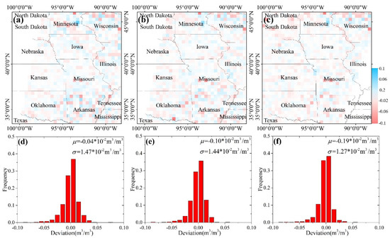
Figure 5.
Comparisons between original and downscaled SM on July 10 (a,d), August 11 (b,e) and October 9 (c,f) in 2017.
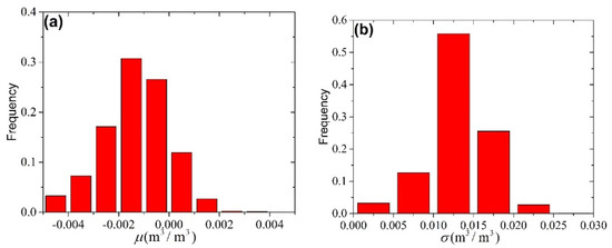
Figure 6.
Statistical histograms of the difference between original and aggregated SM data over the whole study period (2015–2018). (a) Histogram of the mean of the differences μ and (b) histogram of the standard deviation σ of the differences.
4.2. Comparison against in situ SM at CVS
In this section, we evaluated the downscaled SM data against the in situ SM at three CVS stations in Little Washita, Fort Cobb, and South Fork. Figure 7 shows temporal comparisons among the downscaled, original, and in situ SM data. In general, both the downscaled and original SM data are in a good agreement with the in situ SM data. The agreement of both the original and downscaled SM data with in situ SM data is better in Little Washita and Fort Cobb than in South Fork. Land cover type may be one of the main causes for the performance difference [20,46]. The sites of Little Washita and Fort Cobb are dominated by the land cover of grassland, while the South Fork site is mainly covered by cropland.
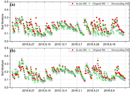
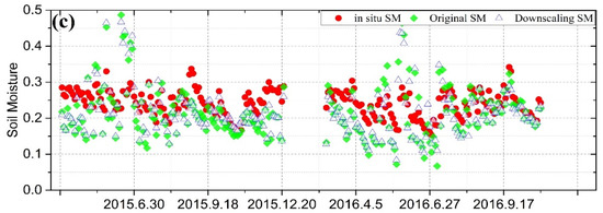
Figure 7.
Comparisons between the original and downscaled SM data against in situ SM measurements at three CVS stations (a) Fort Cobb, (b) Little Washita, and (c) South Fork.
Table 2 shows four evaluation metrics: unbiased root-mean-square error (ubRMSE), root-mean-square error (RMSE), bias (defined as remotely sensed minus in situ data), and correlation coefficient (R) whose calculation equation can be found in [47]. During the evaluation period, the ubRMSE of original SM is 0.028, 0.026, and 0.06 m3/m3 at Fort Cobb, Little Washita and South Fork. The downscaled SM data have very similar ubRMSE values, 0.035, 0.026, and 0.055 m3/m3 at these three sites. The values of R, RMSE, and bias for downscaled SM data in comparison with in situ SM data are also comparable with those of the original SM data. The comparison results suggest that the downscaled SM and original SM data agree very well with in situ SM at the three CVS stations. In other words, our downscaling method preserves the quality of original SM data.

Table 2.
Statistical metrics for the comparison between in situ SM from CVS with concurrent original SM and downscaled SM. FC: Fort Cobb, LW: Little Washita, SF: South Fork. N is the number of comparison samples.
4.3. Comparison against in situ SM at Sparse Stations
The spatial representativeness of in situ SM at network stations may be questionable for validating the remotely sensed SM data. However, these stations cover multiple types of land cover and a larger spatial extent and hence, may provide important supplementary information for evaluating SM data. It should be pointed out that the in situ SM of some network stations are not correlated with original SMAP SM measurements, likely due to the different measurement depth of network stations or too thick vegetation cover. In order to avoid the influence of anomalous SMAP measurements on the downscaling evaluation, we exclude the network stations where the correlation coefficient R of their in situ SM measurements with original SMAP SM is below 0.3.
Figure 8 shows scatter plots of the original/downscaled SM against the in situ SM measurements at the station of SMAP_OK from COSMOS network, MtVernon from SCAN network, and Chillicothe-22-ENE from USCRN network. At the SMAP_OK station, the ubRMSE, RMSE, R and bias are 0.065, 0.032, 0.828, and 0.057 for original SMAP SM data. These metrics are 0.068, 0.032, 0.826, and 0.059 for downscaled SM data, which are very close to those metrics of original SMAP SM data. In addition, we made box plots of original and downscaled SM in comparison with in situ SM measurements at these network stations (Figure 9). The central rectangle box in the box plots spans from the first quartile (Q1) to the third quartile (Q3), and the line segment in the rectangle box indicates the median and the small square symbol in the rectangle box represents the mean. These metrics and box plots show that the performance of the downscale model at the SCAN and USCRN network stations appears similar, but quite different from that at the COSMOS network stations. This may be attributed to the fact that the COSMOS stations measure SM at a depth of about 10–20 cm, whereas the stations of SCAN and USCRN networks measure SM at a depth of 5 cm. In spite of the difference, we found that the downscaled SM and original SMAP SM data have an overall good agreement with in situ SM measurements from the network stations.
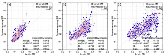
Figure 8.
Scatter plots between the in situ SM measurements against original/downscaled SMAP SM at the network stations (a) COSMOS SMAP_OK, (b) SCAN MtVernon, and (c) USCRN Chillicothe-22-ENE.
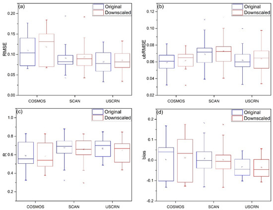
Figure 9.
Box plots of (a) RMSE, (b) ubRMSE, (c) R, and (d) bias between the in situ SM measurements against original/downscaled SMAP SM at all network stations.
5. Discussion
5.1. Influences of Different Downscaling Functions on the DSCALE_mod16 Model
As shown in Equation (5), a cosine-square form [42] was adopted as downscaling function in the proposed DSCALE_mod16 model. In addition to the cosine-square form, two other downscaling functions were frequently used: exponential function [48] and cosine function [49]. In order to estimate the impact of different downscaling functions, we compared the exponential function and cosine function with cosine-square function using the in situ SM measurements at CVS and network stations.
The exponential function and cosine function are given in Equations (8) and (9):
where and represent the volumetric SM. and are the critical SM parameters. Similarly, the critical SM parameter values at coarser resolution can be firstly determined by coarse-resolution SM and coarse-resolution LEE as follows:
where CR denotes the coarse resolution. Then, the critical SM parameters at higher resolution ( and ) can be obtained using the bilinear interpolation method. Finally, the high spatial resolution SM can be obtained by the following equations:
where HR denotes the high resolution. For the exponential form, mathematic error will occur for the pixels where LEE is 1.0. In this study, no-data is set to these pixels in the downscaling SM with exponential function.
Table 3 and Figure 10 show the performances of these three different downscaling functions. As shown in Table 3, the correlation coefficient R of downscaled SM with cosine-square function at all three CVS stations (Fort Cobb, Little Washita, and South Fork) is significantly greater than that with exponential function and cosine function. In addition, RMSE, ubRMSE and bias of the downscaled SM estimates with cosine-square function are lower than with exponential function and cosine function. Therefore, the cosine-square function has the best performance among three candidate downscaling functions for the DSCALE_mod16 model.

Table 3.
Statistical metrics for the comparison between in situ SM from CVS against downscaled SM with three different downscaling functions. The three CVSs are FC: Fort Cobb, LW: Little Washita, and SF: South Fork.
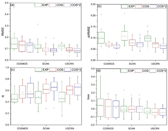
Figure 10.
Box plots of (a) RMSE, (b) ubRMSE, (c) R, and (d) bias between the measured SM against the downscaled SM with three downscaling functions EXP: exponential form, COS: cosine form, and COS^2: cosine-square form based on the statistics over all sparse stations and grouped by their observing networks.
Similar evaluation results are found at network stations. As shown in Figure 10, RMSE, ubRMSE and bias values resulted from the use of cosine-square function are apparently lower than those from the exponential and cosine functions. The R values of the downscaled SM from the cosine-square function are the highest among three candidate downscaling functions. In terms of the mean and median of the four statistical metrics at three network stations, the performance of the cosine-square function is still the best. In summary, our evaluation results suggest that the cosine-square downscaling function is the best choice for the DSCALE_mod16 model.
5.2. Influences of Different LEE Calculation Ways on the DSCALE_mod16 Model
LEE can be defined either as the ratio of latent heat flux (LE) to potential latent heat flux (PLE), or as the ratio of evapotranspiration (ET) to potential ET (PET):
Do the different calculation methods of LEE have a significant impact on the performance of the DSCALE_mod16 model? In order to understand this question, we conducted a comparison between downscaled SM with LEE using the above different calculation ways and in situ measured SM at CVS and sparse networks.
The scatter plots in Figure 11 show the comparisons between the in situ SM measurements at the CVS stations against original and downscaled SMAP SM estimates with two different LEE definitions. The scatter plots clearly show that the downscaled SM estimates using two different LEE definitions are almost identical. The very similar statistical metric values shown in Figure 11 indicate that the impact of two different LEE definitions on the performance of the DSCALE_mod16 model is negligible. Figure 12 shows the comparisons between two different LEE definitions at network stations. The mean, median and histogram distribution of the downscaled SW estimates based on two different LEE definitions are almost the same. Therefore, the use of either the ratio of latent heat flux (LE) to potential latent heat flux (PLE) or the ratio of the evapotranspiration (ET) to potential ET (PET) to define and calculate LEE does not influence the performance of the DSCALE_mod16 model.

Figure 11.
Scatter plots between the in situ measured SM against original/downscaled SM at the CVS of (a) Fort Cobb, (b) Little Washita, and (c) South Fork.
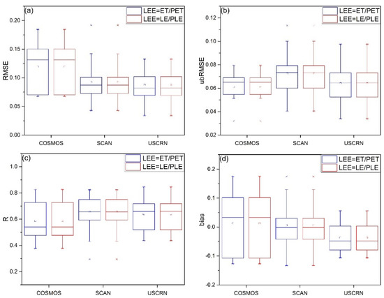
Figure 12.
Comparison between the in situ measured SM against the downscaled SM with two LEE calculation ways using box plots of (a) RMSE, (b) ubRMSE, (c) R, and (d) bias based on the statistics over all sparse stations and grouped by their observing networks.
5.3. Advantages and Uncertainties of the DSCALE_mod16 Model
Most of the optical/thermal and microwave fusion models presented in the previous studies are heavily dependent on the remote sensed LST or LST-derived SMIs. Although LST and LST-derived SMIs are relatively good indicators of the soil moisture status, three major problems hinder their use as the primary downscaling factor. They are the cloud contamination problem in obtaining LST with thermal remote sensing observation, the uncertainty problem in decomposing remotely sensed LST into vegetation and soil components, and the decoupling problem between LST and SM in very dry or very wet condition. Since the completely downscaling process in the DSCALE_mod16 model does not rely on LST or LST-derived SMIs, our DSCALE_mod16 model circumvents the above three problems associated with the optical/thermal & microwave fusion models.
The other advantage is that optical source data used in our model generally have a higher spatial resolution than the thermal infrared data used as the main input in the optical/thermal and microwave fusion models. The MODIS evapotranspiration product MOD16 has a spatial resolution of about 500 m, while the MODIS LST product has a coarser spatial resolution of 1000 m. Compared with the downscaling models that are based on the MODIS LST product, the DSCALE_mod16 model is able to produce higher spatial resolution downscaling estimates.
The SMAP and MOD16 data have different effective temporal resolutions. In order to assimilate them, we assume that spatial distribution of the LEE is invariant during an 8-day interval of MOD16, which may introduce a certain level of uncertainty. Improving the temporal resolution of MODIS ET products (MOD16) is an effective way to reduce this uncertainty. In our current implementation of DSCALE_mod16 model, a barren module with meteorological data was used to fill data gaps of the vegetation module and to obtain full spatial coverage of LEE estimates. The future work could consider other possible gap-filling methods for MODIS ET product.
6. Conclusions
In this study, we presented a spatial downscaling model for disaggregating microwave satellite SM measurements. Our model combines MODIS ET products (MOD16) and a gridded meteorological data to obtain higher spatial resolution LEE as the main downscaling factor to disaggregate microwave remotely sensed SM measurements. The cosine-square downscaling function was the best among three candidate functions to express the quantitative relationship between LEE and SM. The original coarse-resolution SMAP SM and aggregated coarse-resolution LEE were utilized to derive the unknown parameter in the downscaling function. The downscaling function with the determined parameter was then applied to high-resolution LEE to produce high-resolution SM estimates. The LEE can be calculated as the ratio of latent heat flux (LE) to potential latent heat flux (PLE) or the ratio of the evapotranspiration (ET) to potential ET (PET), and either choice does not influence the downscaling results.
In this study, the SMAP L-band passive microwave SM products with a resolution of 36 km were downscaled into SM measurements with a spatial resolution of 500 m using MOD16A2 and GRIDMET data as input. The study area is located in the central United States. The study period spans more than three years from 2015 to 2018. In situ SM measures from three network stations and three CVS stations were used as ground truth to evaluate the downscaling model. Our analysis suggests that the downscaled SM maintains the spatial dynamic range of original SM data while providing more spatial details of SM variation. Moreover, the moisture mass measured from original SMAP observations is conserved during the downscaling process. Using the in situ SM measurements at CVS and network stations, we demonstrated that the downscaled SM and original SMAP SM estimates agree very well with in situ SM measurements. The ubRMSEs of downscaled SM estimates at Fort Cobb, Little Washita and South Fork are comparable to those of original SMAP SM observations. Our downscaling method preserves the quality of original SMAP SM observations, while adding much more spatial variation details.
The major advantage of our DSCALE_mod16 lies in its wide applicability and operational feasibility since it circumvents the “cloud contamination”, “decomposing uncertainty”, and “decoupling effect” problems suffered by most previous downscaling methods. Due to the use of optical remote sensing data as the primary input, our method can generate higher spatial resolution of downscaled SM estimates than the optical/thermal and microwave fusion models that use thermal infrared remote sensing data. Other alternative spatial and temporal gap-filling techniques for MODIS ET products need to be further explored to further improve the performance of the DSCALE_mod16 model.
Author Contributions
Conceptualization, H.S.; methodology, H.S.; formal analysis, B.Z. and C.Z.; writing—Original draft preparation, H.S. and B.Z.; Resources, B.Y. and H.L.; Writing—review and editing, B.Y. and H.L. All authors have read and agreed to the published version of the manuscript.
Funding
This research was funded by National Natural Science Foundation of China, grant number 41871338 and 41771448; Ningxia Key Research and Development Program, grant number 2018BEG03069; Yue Qi Young Scholar Project, CUMTB; and the Fundamental Research Funds for the Central Universities, grant number 2015QD02.
Acknowledgments
The author would like to thank NASA Distributed Active Archive Center at NSIDC and NASA Land Processes Distributed Active Archive Center for providing the SMAP and MODIS data.
Conflicts of Interest
The authors declare no conflict of interest.
References
- Seneviratne, S.I.; Corti, T.; Davin, E.L.; Hirschi, M.; Jaeger, E.B.; Lehner, I.; Orlowsky, B.; Teuling, A.J. Investigating soil moisture-climate interactions in a changing climate: A review. Earth-Sci. Rev. 2010, 99, 125–161. [Google Scholar] [CrossRef]
- Dobriyal, P.; Qureshi, A.; Badola, R.; Hussain, S.A. A review of the methods available for estimating soil moisture and its implications for water resource management. J. Hydrol. 2012, 458, 110–117. [Google Scholar] [CrossRef]
- AghaKouchak, A.; Farahmand, A.; Melton, F.S.; Teixeira, J.; Anderson, M.C.; Wardlow, B.D.; Hain, C.R. Remote sensing of drought: Progress, challenges and opportunities. Rev. Geophys. 2015, 53, 452–480. [Google Scholar] [CrossRef]
- Sun, H.; Zhao, X.; Chen, Y.H.; Gong, A.D.; Yang, J. A new agricultural drought monitoring index combining modis ndwi and day-night land surface temperatures: A case study in china. Int. J. Remote Sens. 2013, 34, 8986–9001. [Google Scholar] [CrossRef]
- Pablos, M.; Martinez-Fernandez, J.; Sanchez, N.; Gonzalez-Zamora, A. Temporal and spatial comparison of agricultural drought indices from moderate resolution satellite soil moisture data over northwest spain. Remote Sens. 2017, 9, 1168. [Google Scholar] [CrossRef]
- Robinson, D.A.; Campbell, C.S.; Hopmans, J.W.; Hornbuckle, B.K.; Jones, S.B.; Knight, R.; Ogden, F.; Selker, J.; Wendroth, O. Soil moisture measurement for ecological and hydrological watershed-scale observatories: A review. Vadose Zone J. 2008, 7, 358–389. [Google Scholar] [CrossRef]
- Dai, A.; Trenberth, K.E.; Qian, T.T. A global dataset of palmer drought severity index for 1870−2002: Relationship with soil moisture and effects of surface warming. J. Hydrometeorol. 2004, 5, 1117–1130. [Google Scholar] [CrossRef]
- Anderson, M.C.; Norman, J.M.; Mecikalski, J.R.; Otkin, J.A.; Kustas, W.P. A climatological study of evapotranspiration and moisture stress across the continental united states based on thermal remote sensing: 2. Surface moisture climatology. J. Geophys. Res.-Atmos. 2007, 112, 13. [Google Scholar] [CrossRef]
- WMO. Essential Climate Variables. Available online: https://public.wmo.int/en/programmes/global-climate-observing-system/essential-climate-variables (accessed on 17 December 2018).
- Petropoulos, G.P.; Ireland, G.; Barrett, B. Surface soil moisture retrievals from remote sensing: Current status, products & future trends. Phys. Chem. Earth 2015, 83–84, 36–56. [Google Scholar]
- Crow, W.T.; Berg, A.A.; Cosh, M.H.; Loew, A.; Mohanty, B.P.; Panciera, R.; de Rosnay, P.; Ryu, D.; Walker, J.P. Upscaling sparse ground-based soil moisture observations for the validation of coarse-resolution satellite soil moisture products. Rev. Geophys. 2012, 50, RG2002. [Google Scholar] [CrossRef]
- Peng, J.; Loew, A.; Merlin, O.; Verhoest, N.E.C. A review of spatial downscaling of satellite remotely sensed soil moisture. Rev. Geophys. 2017, 55, 341–366. [Google Scholar] [CrossRef]
- Colliander, A.; Fisher, J.B.; Halverson, G.; Merlin, O.; Misra, S.; Bindlish, R.; Jackson, T.J.; Yueh, S. Spatial downscaling of smap soil moisture using modis land surface temperature and ndvi during smapvex15. IEEE Geosci. Remote Sens. Lett. 2017, 14, 2107–2111. [Google Scholar] [CrossRef]
- Wu, X.; Walker, J.P.; Das, N.N.; Panciera, R.; Rüdiger, C. Evaluation of the smap brightness temperature downscaling algorithm using active–passive microwave observations. Remote Sens. Environ. 2014, 155, 210–221. [Google Scholar] [CrossRef]
- NASA. Smap Handbook-Soil Moisture Active Passive; Mapping Soil Moisture Freeze/Thaw from Space: Pasadena, CA, USA, 2014. [Google Scholar]
- Kerr, Y.H.; Waldteufel, P.; Wigneron, J.; Delwart, S.; Cabot, F.; Boutin, J.; Escorihuela, M.; Font, J.; Reul, N.; Gruhier, C.; et al. The smos mission: New tool for monitoring key elements of the global water cycle. Proc. IEEE 2010, 98, 666–687. [Google Scholar] [CrossRef]
- Entekhabi, D.; Njoku, E.G.; Neill, P.E.O.; Kellogg, K.H.; Crow, W.T.; Edelstein, W.N.; Entin, J.K.; Goodman, S.D.; Jackson, T.J.; Johnson, J.; et al. The soil moisture active passive (smap) mission. Proc. IEEE 2010, 98, 704–716. [Google Scholar] [CrossRef]
- Pablos, M.; Martínez-Fernández, J.; Piles, M.; Sánchez, N.; Vall-llossera, M.; Camps, A. Multi-temporal evaluation of soil moisture and land surface temperature dynamics using in situ and satellite observations. Remote Sens. 2016, 8, 587. [Google Scholar] [CrossRef]
- Molero, B.; Merlin, O.; Malbéteau, Y.; Al Bitar, A.; Cabot, F.; Stefan, V.; Kerr, Y.; Bacon, S.; Cosh, M.H.; Bindlish, R.; et al. Smos disaggregated soil moisture product at 1 km resolution: Processor overview and first validation results. Remote Sens. Environ. 2016, 180, 361–376. [Google Scholar] [CrossRef]
- Sun, H.; Zhou, W.; Zhang, Y.; Cai, C.; Chen, Q. Integrating spectral and textural attributes to measure magnitude in object-based change vector analysis. Int. J. Remote Sens. 2019, 40, 5747–5767. [Google Scholar] [CrossRef]
- Chan, S.K.; Bindlish, R.; O’Neill, P.; Jackson, T.; Njoku, E.; Dunbar, S.; Chaubell, J.; Piepmeier, J.; Yueh, S.; Entekhabi, D.; et al. Development and assessment of the smap enhanced passive soil moisture product. Remote Sens. Environ. 2018, 204, 931–941. [Google Scholar] [CrossRef]
- Chauhan, N.S.; Miller, S.; Ardanuy, P. Spaceborne soil moisture estimation at high resolution: A microwave-optical/ir synergistic approach. Int. J. Remote Sens. 2003, 24, 4599–4622. [Google Scholar] [CrossRef]
- Srivastava, P.K.; Han, D.; Ramirez, M.R.; Islam, T. Machine learning techniques for downscaling smos satellite soil moisture using modis land surface temperature for hydrological application. Water Resour. Manag. 2013, 27, 3127–3144. [Google Scholar] [CrossRef]
- Piles, M.; Camps, A.; Vall-llossera, M.; Corbella, I.; Panciera, R.; Rudiger, C.; Kerr, Y.H.; Walker, J. Downscaling smos-derived soil moisture using modis visible/infrared data. IEEE Trans. Geosci. Remote Sens. 2011, 49, 3156–3166. [Google Scholar] [CrossRef]
- Kim, J.; Hogue, T.S. Improving spatial soil moisture representation through integration of amsr-e and modis products. IEEE Trans. Geosci. Remote Sens. 2012, 50, 446–460. [Google Scholar] [CrossRef]
- Sun, H. Two-stage trapezoid: A new interpretation of the land surface temperature and fractional vegetation coverage space. IEEE J. Sel. Top. Appl. Earth Obs. Remote Sens. 2016, 9, 336–346. [Google Scholar] [CrossRef]
- Jiang, L.; Islam, S. An intercomparison of regional latent heat flux estimation using remote sensing data. Int. J. Remote Sens. 2003, 24, 2221–2236. [Google Scholar] [CrossRef]
- Peng, J.; Loew, A.; Zhang, S.; Wang, J.; Niesel, J. Spatial downscaling of satellite soil moisture data using a vegetation temperature condition index. IEEE Trans. Geosci. Remote Sens. 2016, 54, 558–566. [Google Scholar] [CrossRef]
- Peng, J.; Niesel, J.; Loew, A. Evaluation of soil moisture downscaling using a simple thermal-based proxy–the remedhus network (spain) example. Hydrol. Earth Syst. Sci. 2015, 19, 4765–4782. [Google Scholar] [CrossRef]
- Merlin, O.; Al Bitar, A.; Walker, J.P.; Kerr, Y. An improved algorithm for disaggregating microwave-derived soil moisture based on red, near-infrared and thermal-infrared data. Remote Sens. Environ. 2010, 114, 2305–2316. [Google Scholar] [CrossRef]
- Merlin, O.; Rudiger, C.; Al Bitar, A.; Richaume, P.; Walker, J.P.; Kerr, Y.H. Disaggregation of smos soil moisture in southeastern australia. IEEE Trans. Geosci. Remote Sens. 2012, 50, 1556–1571. [Google Scholar] [CrossRef]
- Sun, H.; Wang, Y.M.; Liu, W.H.; Yuan, S.Y.; Nie, R.W. Comparison of three theoretical methods for determining dry and wet edges of the lst/fvc space: Revisit of method physics. Remote Sens. 2017, 9, 15. [Google Scholar]
- Petropoulos, G.; Carlson, T.N.; Wooster, M.J.; Islam, S. A review of ts/vi remote sensing based methods for the retrieval of land surface energy fluxes and soil surface moisture. Prog. Phys. Geogr. Earth Environ. 2009, 33, 224–250. [Google Scholar] [CrossRef]
- Carlson, T. An overview of the “triangle method” for estimating surface evapotranspiration and soil moisture from satellite imagery. Sensors 2007, 7, 1612. [Google Scholar] [CrossRef]
- Long, D.; Singh, V.P. A two-source trapezoid model for evapotranspiration (ttme) from satellite imagery. Remote Sens. Environ. 2012, 121, 370–388. [Google Scholar] [CrossRef]
- Wang, D.; Chen, Y.; Cui, Y.; Sun, H. A geometric model to simulate urban thermal anisotropy for simplified neighborhoods. IEEE Trans. Geosci. Remote Sens. 2018, 56, 4930–4944. [Google Scholar] [CrossRef]
- Yao, Y.J.; Liang, S.L.; Qin, Q.M.; Wang, K.C.; Zhao, S.H. Monitoring global land surface drought based on a hybrid evapotranspiration model. Int. J. Appl. Earth Obs. Geoinf. 2011, 13, 447–457. [Google Scholar] [CrossRef]
- Anderson, M.C.; Hain, C.; Wardlow, B.; Pimstein, A.; Mecikalski, J.R.; Kustas, W.P. Evaluation of drought indices based on thermal remote sensing of evapotranspiration over the continental united states. J. Clim. 2011, 24, 2025–2044. [Google Scholar] [CrossRef]
- Mu, Q.Z.; Zhao, M.S.; Kimball, J.S.; McDowell, N.G.; Running, S.W. A remotely sensed global terrestrial drought severity index. Bull. Am. Meteorol. Soc. 2013, 94, 83–98. [Google Scholar] [CrossRef]
- Choi, M.; Jacobs, J.M.; Anderson, M.C.; Bosch, D.D. Evaluation of drought indices via remotely sensed data with hydrological variables. J. Hydrol. 2013, 476, 265–273. [Google Scholar] [CrossRef]
- Fisher, J.B.; Tu, K.P.; Baldocchi, D.D. Global estimates of the land–atmosphere water flux based on monthly avhrr and islscp-ii data, validated at 16 fluxnet sites. Remote Sens. Environ. 2008, 112, 901–919. [Google Scholar] [CrossRef]
- Lee, T.J.; Pielke, R.A. Estimating the soil surface specific humidity. J. Appl. Meteorol. 1992, 31, 480–484. [Google Scholar] [CrossRef]
- Abatzoglou, J.T. Development of gridded surface meteorological data for ecological applications and modelling. Int. J. Climatol. 2013, 33, 121–131. [Google Scholar] [CrossRef]
- Dorigo, W.; Wagner, W.; Hohensinn, R.; Hahn, S.; Paulik, C.; Xaver, A.; Gruber, A.; Drusch, M.; Mecklenburg, S.; Oevelen, P.v. The international soil moisture network: A data hosting facility for global in situ soil moisture measurements. Hydrol. Earth Syst. Sci. 2011, 15, 1675–1698. [Google Scholar] [CrossRef]
- Colliander, A. Smap/In Situ Core Validation Site Land Surface Parameters Match-Up Data, version 1; NASA National Snow and Ice Data Center Distributed Active Archive Center: Boulder, CO, USA, 2017. [Google Scholar]
- Colliander, A.; Jackson, T.J.; Bindlish, R.; Chan, S.; Das, N.; Kim, S.B.; Cosh, M.H.; Dunbar, R.S.; Dang, L.; Pashaian, L.; et al. Validation of smap surface soil moisture products with core validation sites. Remote Sens. Environ. 2017, 191, 215–231. [Google Scholar] [CrossRef]
- Portal, G.; Vall-llossera, M.; Piles, M.; Camps, A.; Chaparro, D.; Pablos, M.; Rossato, L. A spatially consistent downscaling approach for smos using an adaptive moving window. IEEE J. Sel. Top. Appl. Earth Obs. Remote Sens. 2018, 11, 1883–1894. [Google Scholar] [CrossRef]
- Komatsu, T.S. Toward a robust phenomenological expression of evaporation efficiency for unsaturated soil surfaces. J. Appl. Meteorol. 2003, 42, 1330–1334. [Google Scholar] [CrossRef]
- Noilhan, J.; Planton, S. A simple parameterization of land surface processes for meteorological models. Mon. Weather Rev. 1989, 117, 536–549. [Google Scholar] [CrossRef]
© 2020 by the authors. Licensee MDPI, Basel, Switzerland. This article is an open access article distributed under the terms and conditions of the Creative Commons Attribution (CC BY) license (http://creativecommons.org/licenses/by/4.0/).