Multi-Label Remote Sensing Image Classification with Latent Semantic Dependencies

Abstract

Deforestation in the Amazon rainforest results in reduced biodiversity, habitat loss, climate change, and other destructive impacts. Hence obtaining location information on human activities is essential for scientists and governments working to protect the Amazon rainforest. We propose a novel remote sensing image classification framework that provides us with the key data needed to more effectively manage deforestation and its consequences. We introduce the attention module to separate the features which are extracted from CNN(Convolutional Neural Network) by channel, then further send the separated features to the LSTM(Long-Short Term Memory) network to predict labels sequentially. Moreover, we propose a loss function by calculating the co-occurrence matrix of all labels in the dataset and assigning different weights to each label. Experimental results on the satellite image dataset of the Amazon rainforest show that our model obtains a better $F_2$ score compared to other methods, which indicates that our model is effective in utilizing label dependencies to improve the performance of multi-label image classification.

1. Introduction

Deforestation in the Amazon rainforest has become a severe issue in the past decades, causing devastating impacts on the ecosystems and the environment. Therefore, tracking changes in the rainforest and better analyzing the location of human encroachment on forests are needed, which can help people stop deforestation and protect the earth.

The advancement achieved recently in satellite technology has led to significant growth of RS image archives. RS images contain more detailed features of ground objects and more complex spectral features than ordinary images. Therefore, RS images have more applications in many fields. They can be used for smart and connected communities [1]. By distinguishing the spectral characteristics of different materials, RS image information can be used for monitoring floods [2], typhoons and torrential rains [3], forecasting earthquakes and tsunamis [4], tracking ships [5], monitoring forestry [6] and the effects of climate change [7], etc.

In real-world classification tasks, since images contain rich semantic information, it is often necessary to assign multiple labels to each instance. Multi-label image classification is more widely used than single-label image classification, such as image retrieval, image annotation, scene recognition, etc. These applications need to model rich semantic information and their dependencies which is challenging, consequently it is essential to learn multiple semantic features and classify images with multi-labels.

Since AlexNet [8] has achieved good results on ImageNet [9], CNNs have been used in image classification broadly. Zhao et al. [10] used multi-scale two-dimensional CNN (2d-CNN) to deeply present remote sensing images and integrate multi-band spectral information for classification. However, different feature extraction scales need to be designed, and feature areas may confuse objects of different shapes and types. Maggiori et al. [11] came up with a framework based on CNNs which is end-to-end to classify satellite images in pixel level. However, these methods ignore the potential semantic dependencies between labels. Mou et al. [12] introduced a method based on RNN(Recurrent Neural Network) to classify images, demonstrating the potential of the deep recursive network to utilize label correlation in classification tasks. Therefore, people try to combine CNN and RNN to make better use of semantic dependence to improve classification performance. However, most of the methods mentioned above are designed for single-label classification. Since multi-label images can be regarded as an extension of single-label images, we consider applying the method of solving single-label image classification to the task of multi-label image classification.

In this paper, we propose a innovative framework that makes full use of the characteristics of the LSTM model.It subjects to the ”Encoder-Decoder” design pattern, CNN is used for encoding, and RNN is used for decoding. The CNN model uses DenseNet121-BC to extract features from the given images, then model channels and labels with attention module, lastly using the LSTM to generate an associated image label sequence. The contributions of this paper can be summarized as follows:

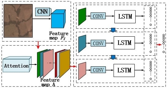
• We propose a novel framework for multi-label remote sensing image classification. By introducing the attention module into the CNN-RNN structure, the RNN can notice some small targets which might be neglected and easier to extract the correlation between labels.
• We propose a new loss function, which solves the problem of imbalance in the proportion of labels in the dataset. It helps to improve the classification results of rare labels, thereby improving the overall classification performance.
• We conduct experiments and evaluations on the dataset of the Amazon rainforest and prove that our proposed model is superior to other leading multi-label image classification methods in $F_2$ scores.

The rest of the paper proceeds as follows. The Section 2 briefly introduces several methods of multi-label image classification, and the Section 3 describes the model in detail and the pre-processing for our task. The Section 4 introduces the dataset for multi-label classification task of remote sensing images, the corresponding experiment and experimental results. Finally, conclusions are given in the Section 5.

2. Related Works

Remote sensing images contain rich band information, which can show complex ground features and meteorological features. The information extracted from these features is very crucial for subsequent analysis and application. Xu et al. improve pixel-level detection method, which can more accurately detect changes in RS images [13]. Peng et al. [14] trained a nonlinear kernel function expression using the Ideal Regularization Kernel, and then combined it with Support Vector Machine for classification. However, as the data increases, the kernel function becomes insufficient to express the nonlinear relationship between the data and its labels. Fang et al. [15] proposed an unsupervised RS image classification method using Hidden Markov Random Field (HMM). Yao et al. [16] proposed using the Stacked AutoEncoder(SAE) to extract features from images. The above two methods can automatically classify images, but good accuracy can only be achieved when the categories are small.

In recent years, the multi-label classification has attracted the attention of many researchers and various effective methods are proposed. For example, the bag-of-words (BOW) [17,18,19,20] which extracts features such as Scale Invariant Feature Transform(SIFT) [21], Histogram of Oriented Gradient(HOG) [22], Local Binary Pattern(LBP) [23] manually, Support Vector Machine(SVM) [24], random forests [25] ) and context modeling [17,18] were proposed. Since CNNs have achieved great success recent years, Chat-field et al. adjusted the network to adapt to new tasks with the pre-trained CNN model on ImageNet, reducing the time and the difficulty of training. Gong et al. [26] concluded that top-k ranking loss worked greatest among several loss functions with CNNs. Li et al. [27] put forward a modern loss function which makes the deep network converge faster and easier to optimize. In order to reduce the defect that the experimental results are greatly influenced by complex background, Yang et al. [28] used the region proposals to extract the information area of the images effectively.

To model the label dependencies, RNN was introduced into the multi-label classification task. Wang et al. [29] proposed a model that exploits the characteristic of memory in RNN [30,31] to explore the relevance of the labels. In the model mentioned above, the ability of the model cannot be fully utilized based on VGG(Visual Geometry Group Network) for feature extraction. Therefore, Zhang et al. [32] made improvements in the component CNN. Our proposed method is also based on the CNN-RNN model. Unlike [28], the channels of the feature map are separated through attention module, making the LSTM can pay more attention to some small size targets and capture the dependencies between the labels to improve performance.

The attention module plays an significant role in computer vision, which has benefited many vision tasks. For example, image classification [33,34], and image captioning [35]. Work [33] build a recurrent attention model utilizing the attention module, and successfully applied it to the classification tasks with low-resolution images. Feng et al. [34] used attention heatmap to explore spatial relations between labels and thus virtually improving classification performance. The attention module have been confirmed beneficial in label dependencies learning.

3. Methodology

The multi-label image classification task is defined as a problem of generating labels sequentially and predict all possible labels for a given image. Given the image training set $X=\{x_1,x_2,...,x_N\}$ and the corresponding label $Y=\{y_1,y_2,...y_N\}$, where N represents the number of training images. The corresponding label of the i-th image $x_i$ is $y_i=y_{i1},y_{i2},..y_{iC}$, where C represents the number of labels; $y_{ij}=1$ represents that the image $x_i$ contains the label j, otherwise $y_{ij}=0$. Build an end-to-end model and learn the mapping from image to label $f:X$→Y. At the time of testing, an image is given, and a plurality of labels corresponding to the image are predicted by mapping f.

Our model consists of three subsections: DenseNet121- BC, attention module, and LSTM network. Figure 1 illustrates the overall architecture of our model. The model is based on the CNN-RNN structure and treats multiple labels of an image as a sequence. The feature $F_I$ is extracted from the image using DenseNet. In order to take full advantages of the characteristics of the deep neural network, features are extracted from the last layer of the fully connected layer. Attention module is used to separate features of different targets, and the LSTM decodes the channels of these feature maps to predict the labels.

3.1. Densenet for Feature Extraction

Because of the different scales and semantics of the labels to predict, DenseNet is an excellent choice for feature extraction. DenseNet is composed of dense blocks. The dense blocks are composed of a stack of convolutional layers which make each dense layer can receive features from all previous dense layers. This design allows the high-level layer to directly access all the information of the previous layers, which facilitates the use of the classifier to access the information from different layers of the architecture for label prediction. And accordingly we use DenseNet121-BC as the feature extraction network. The DenseNet121-BC network has 121 layers, which is enough to handle the classification task. B(Bottleneck)C(Compression) indicates that the model uses the bottleneck layer and the compression ratio is greater than 0. As described in [7], the bottleneck layer and compression can improve the computational efficiency. Given an image $x_n$, We use DenseNet121-BC to extract the features of the image which can be formulated as:

$$F_I=CNN\left(x_n\right)$$

(1)

$F_I$ is the output feature map of the DenseNet121-BC. In DenseNet121-BC, the input image size is 224 × 224, the corresponding output feature map size is 7 × 7, which is further sent to the attention module to model the relation between labels and channels.

3.2. Attention Module

In order to exploit the semantic dependencies between multiple labels of an image, RNN is introduced to improve the classification performance. If directly input the feature maps output by DenseNet into the LSTM network, the feature map at this time contains multiple objects so that the LSTM cannot only focus on the exploration of label correlation. Therefore, the attention module is used to separate the features of different targets in the channel dimension of the feature map. By sending separated channels one by one into the LSTM network, LSTM can focus on capturing dependencies between labels and improving recognition performance. Given the input feature map $F_I\in R^{7\times 7\times C}$, generate the attention values for each label:

$$Z=Con{v}_{att}\left(F_I\right),Z\in R^{7\times 7\times C}$$

(2)

where Z is the unnormalized label attention value, and each channel corresponds to one label. Spatial normalization of Z using the softmax function to obtain the final attention map A:

$$a_{i,j}^l=\frac{exp\left(z_{i,j}^l\right)}{{\sum }_{i,j}exp\left(z_{i,j}^l\right)},A\in R^{7\times 7\times C}$$

(3)

where $z_{i,j}^l$ and $a_{i,j}^l$ represent the unnormalized and normalized attention values at $(i,j)$ of the $l-th$ channel.

Each image has only one or several labels, but each channel has responses to each class. The responses for labels that do not exist have a negative impact on labels prediction. In order to suppress negative impacts, we introducing a confidence map S to learn spatial regularizations from weighted attention maps $U\in R^{7\times 7\times C}$,

$$U=\sigma \left(S\right)\otimes A,U\in R^{7\times 7\times C}$$

(4)

where $\sigma (·)=1/(1+e^{-·})$ normalizes label confidences S to the range (0,1), and ⊗ represents the element-wise multiplication. U is a weighted attention map of the A. The attention module is used to separate the features of different targets of the feature map, so that the channel corresponds to the label, and the feature map channel is sequentially fed to the LSTM for decoding.

3.3. Lstm for Latent Semantic Dependencies

LSTM is a type of RNN that has a strong ability to handle sequence problems. LSTM not only predicts labels based on features, but also captures latent semantic dependencies between labels. LSTM extends RNN by adding three control gates to an RNN neuron: a forget gate, an input gate and an output gate. They respectively control whether to forget the current state, whether to obtain the information of current input and whether to output the state. These three gates enable LSTM to perform well in both long-term and short-term sequence and make the model easier to optimize. Figure 2 is the basic structure of LSTM. The LSTM update progress for time step t can be expressed as:

$$m_t=tanh(W_{xc}{x}_t+W_{hc}{h}_{t-1}+b_c)$$

(5)

$$i_t=\sigma (W_{xi}{x}_t+W_{hi}{h}_{t-1}+b_i)$$

(6)

$$f_t=\sigma (W_{xf}{x}_t+W_{hf}{h}_{t_1}+b_f)$$

(7)

$$o_t=\sigma (W_{xo}{x}_t+W_{ho}{h}_{t-1}+b_o)$$

(8)

$$c_t=f_t\otimes c_{t-1}+i_t\otimes m_t$$

(9)

$$h_t=o_t\times tanh\left(c_t\right)$$

(10)

where all of the W and b represent the parameters to be trained, and $x_t$ represents the input at time t. $i_t$, $f_t$ and $o_t$ represent the output of the input, forget and output gates in the LSTM, respectively. $c_t$ and $h_t$ represent the memory and the hidden state of the LSTM. $\sigma (·)$ is the sigmoid activation function.

We can see that LSTM uses its structure to capture the relevance of labels by the storage unit encodes useful information at each time step. When predicting the label corresponding to the channel of each feature map, $c_t$ fuses the correlation of the labels of all the previous channels, thus, the recognition ability of the current prediction label can be easily improved.

Each channel of the feature map corresponds to one label that allows the LSTM network to focus on capturing semantic dependencies between labels. To be specific, first to encode the channel $v_t$, and the obtained result $x_t$ is then fed to the LSTM one by one to obtain the predicted probability of the label $p_t$:

$$x_t=relu(W_{vx}{v}_t+b_x)$$

(11)

$$h_t=LSTM(x_t,h_{t-1},c_{t-1})$$

(12)

$$p_t=\sigma (W_{hp}{h}_t+b_h)$$

(13)

where $W_{vx}$ and $b_x$ are the convolutional parameters, and $W_{hp}$ and $b_h$ are the classification layer parameters.

3.4. Max-Pooling and Loss Function

After $K+1$ iterations, the score vector $\left\{s_1,s_2,...,s_K\right\}$ of the LSTM output is obtained, where $s_k=\left\{s_k^1,s_k^2,...,s_k^C\right\}$ denotes the scores over C class labels. We use the category-wise max-pooling method to get the final label probability value $s=\left\{s^1,s^2,...,s^C\right\}$:

$$s^i=max(s_1^i,s_2^i,...,s_K^i),i\in (1,2,...,C)$$

(14)

Since an image may correspond to several labels, but the objects corresponding to these labels occupy different proportions in the images. In order to deal with the imbalance, we propose a new loss function. Firstly, we calculate the co-occurrence matrix of all the labels on the whole training set. The ground-true probability vector of the $i-th$ sample is defined as $\widehat{p_i}$. Then given the predicted probability vector $p_i$:

$$P_i^c=\frac{exp\left(s_i^c\right)}{{\sum }_{c^{\prime }=1}^{C}exp\left(s_i^c\right)},c=1,2,...,C$$

(15)

The classification loss function is defined as:

$$L_{cls}=-\frac{1}{N}\sum _{j=1}^N\sum _{c=1}^C{a}_i{(\widehat{p_i^c}-p_i^c)}^2$$

(16)

where $a_i$ is calculated from the co-occurrence matrix of all the labels on the training set. Assuming that the label set of an image is L, we acquire a set Q, which are the probabilities of labels in L appear together according to the co-occurrence matrix. The weight of $a_i$ of each label in L is calculated as:

$$a_i=\frac{q_i}{{\sum }_{j=1}^L{q}_j}$$

(17)

3.5. Data Augmentation

To improve generalization and prevent overfitting, we apply various modifications to increase the diversity of the training images called augmentation.

• The size of original images from our dataset is 256 × 256, they are then cropped to 224 × 224 to fit the network input size. We take five crops for each image(four in the corners and one in the center);
• Unlike ordinary images such as what is in the ImageNet, satellite images can preserve semantic information after flipping and rotation, accordingly we applied both horizontal and vertical flips;
• We rotate each image to 90, 180, and 270 degrees.

In this way, we transform each image into 6 × 2 × 3 = 36 training samples. In training, we randomly pick 1 of the 36 transformations for each image in each epoch. In the test period, we only use the images which obtain complete image information. These transformations make our model more robust and ameliorate the poor performance on rare features.

4. Experiment

4.1. Dataset

We use the data from the kaggle competition ”Planet: Understanding the Amazon from Space”. It is a satellite remote sensing image of the Amazon rainforest from Planet Flock2 satellite from January 2016 to January 2017. The spatial resolution is 3.7 m and the resolution of the image is 256 × 256. The dataset contains 40,479 labelled training images and 61,192 unlabelled images. We randomly selected the 20% (8096) of the labelled images for training, and then 20% (8096) of the labelled images for validation, the rest is used for training. Each image has up to 17 labels, and these labels can be approximately divided into three categories: four atmosphere condition labels ( haze, cloudy, partly_cloudy, clear), six land condition labels ( water, habitation, agriculture, cultivation, road, primary) and seven rare labels ( bare_ground, artisinal_mine, slash_burn, conventional_mine, selective_logging, blooming, blow_down). We randomly select 8 images as shown in Figure 3.

Figure 4 shows the label distribution of the images from dataset. It can be seen that the distribution of the label is severely skewed, and the frequency of the labels appears from more than 90% (primary) to less than 1% (i.e., blow_down, conventional_mine, slash_burn, blooming, artisanal_mine, selective_logging, etc.). There may be an under-fitting problem due to the small number of rare labels. Therefore, proper data augmentation can improve the performance of classification.

The co-occurrence matrix can provide a large amount of information for multi-label classification. Figure 5 is a heat map of the co-occurrence matrix between different labels. If we narrow down the heat map, we can see that each image can only have one of the four atmosphere condition labels, but the land condition labels and the rare labels may overlap. For example, the primary and agriculture, agriculture and water have a trend to occur together. Therefore, we hope to explore the potential relevance of image labels through LSTM to improve the performance of classification.

4.2. Evaluation

In this paper, the $F_2$ score is used as the evaluation standard of experimental results. Calculated as follows:

$$F_2=(1+{\beta }^2)\frac{p·r}{{\beta }^{2}p+r},p=\frac{tp}{tp+fp},r=\frac{tp}{tp+fn},\beta =2$$

(18)

Where p is the precision of the predicted set of labels and r is the recall. $tp$, $fp$, and $fn$ represent the number of true positives, the number of false positives, and the number of false negatives, respectively. $\beta$ represents weights that are used to balance the importance of precision and recall.

4.3. Classification Performance

Unfortunately, when directly using our model to classify images after data augmentation, the obtained classification results are not good compared with the excellent results that already exist. Because the number of our dataset is not enough, especially the rare labels, the weights can not converge to their optimal values when training from scratch. To solve this problem, we use a training method based on transfer learning. Transfer learning refers to migrating already trained model parameters to a new model. ImageNet is a vast dataset and there are already some deep architectures trained on it which are a good source of pre-trained models for other classification problems. Thus, we regard the CNN model pre-trained on the ImageNet dataset as the starting point for our model. Specifically, we make the last fully connected layer of Densenet121-BC adapted to our task. Use a learning rate of 0.001 to train this layer for ten epochs with all convolutional layers frozen, then training all layers using a smaller learning rate to fine-tune the parameters of both the CNN and the fully connected layer.

Based on the above training method, we use several models to classify RS images on the dataset. The baseline CNN contains three convolutional layers followed by two fully connected layers, and every convolutional layer used a ReLU nonlinearity, batch-norm and max-pooling layer.

Table 1. The $m.F_2$ score for each model on training, validation and test set. $m.F_2$ refers to the average of $F_2$ scores obtained from 20 repeated experiments. And all the standard deviation(std) is less than 0.01.

Networks	Training $\mathit{m}.{\mathit{F}}_2$	Validition $\mathit{m}.{\mathit{F}}_2$	Test $\mathit{m}.{\mathit{F}}_2$
baseline	0.859	0.851	0.849
VGG16	0.915	0.912	0.909
ResNet-50	0.921	0.917	0.915
VGG16-LSTM	0.918	0.914	0.913
ResNet50-LSTM	0.924	0.920	0.919
DenseNet121-LSTM	0.926	0.923	0.922

provides the $F_2$ scores for each model on the training, validation andte set and the validation set.

From Table 1, we can find that the results of models based on convolutional networks are good. The results of baseline CNN is not bad, but as the depth of the network increases, the classification performs better, indicating that the depth of the model has a great impact on the multi-label classification. Our model obtained the highest $F_2$ score among these models, which is mainly due to the use of the dependencies between labels and selecting the DenseNet network as the feature extractor. By exploiting the dependencies between labels, some rare labels may be predicted accordingly based on other predicted labels. The DenseNet architecture allows each block to get information from the previous blocks, and this characteristic matches the task for generating labels sequentially, the prediction of the current label needs the information from the previous labels.

We plot the co-occurrence matrix of the real labels and the prediction labels on the validation set as shown in Figure 6. It is not difficult to find that the two figures are very similar, indicating that our model has predicted the correlation between labels very well. Figure 6 shows that the plot on the right side is lighter than the left. Because the model is more inclined to predict more positive than the basic fact, the classifier tends to predict more labels to conservatively reduce its losses, even if there are fakes in the labels. This strategy can also be verified from a fast and stable loss curve. From Figure 6, we see that the model successfully captured some relationships between the labels.

Figure 7 shows a few examples on which we use to generate predictions. For the first row, we successfully predicted all the labels for the leftmost image: agriculture, haze, primary, road and water. In the next image, we also successfully predicted all the labels including the rare label blooming, which verified the effectiveness of our model in modeling the label dependencies. The middle image in the second row also successfully predicted all the labels, indicating that the model is very effective for predicting non-rare labels. The rightmost images of both rows successfully predicted all the labels, respectively are agriculture, cultivation, partial_cloudy, primary and agriculture, habitation, partly_cloudy, primary, road, illustrating the superiority of the model which can accurately predict the labels. For the leftmost image of the second row, we predicted clear, primary, bare_ground, slash_burn, but failed to predict the label blow_burn, erroneously predicted the conventional_mine, indicating that the model has some difficulty in predicting particularly rare labels.

Figure 8 gives a loss curve of our model during 20 training epochs and the $F_2$ convergence curves during the training and validation periods. The increase in training epochs correspond to the decreases in the training loss and the increases in $F_2$ scores, and the $F_2$ score at the time of validation does not decrease significantly compared with the training period, suggesting that our model does not suffer from overfitting. Therefore, in the process of further improving the classification performance, we can consider increasing the model complexity and other model optimization methods to improve the $F_2$ score.

The $F_2$ score distribution for each of the labels shown in Figure 9 is similar to the frequency distribution of the labels shown in Figure 4. This is reasonable because more data allows the model to learn more features for better results. Labels with a small number of visual differences in different samples, such as bare ground, selective_logging, conventional_mine, blooming, blow_down, slash_burn, etc., have significantly lower $F_2$ scores due to severe under-fitting. It can be seen that the differences in the samples and the imbalance of the data have a significant impact on the multi-label image classification. Consequently, it is possible to improve performance by increasing the frequencies of the rare labels in the training set.

5. Conclusions

In this paper, a multi-label classification model Densenet121-LSTM is proposed for RS images. All experiments on the RS image dataset of the Amazon rainforest are under the same experimental conditions, compared with several multi-label classification models based on CNN, our method achieves the best test $F_2$ score.

In the future, in order to make the classification performs better, we can improve from the following aspects: optimize and adjust the network structure to get a better test $F_2$ score; use Generative Adversarial Nets (GAN) to generate new training samples and replace traditional data augmentation methods to increase the proportion of rare landmarks.

References

1. Sun, Y.; Song, H.; Jara, A.J.; Bie, R. Internet of things and big data analytics for smart and connected communities. IEEE Access 2016, 4, 766–773. [Google Scholar] [CrossRef]
2. Refice, A.; Capolongo, D.; Pasquariello, G.; D’Addabbo, A.; Bovenga, F.; Nutricato, R.; Lovergine, F.P.; Pietranera, L. Sar and insar for flood monitoring: Examples with cosmo/skymed data. IEEE J. Sel. Top. Appl. Earth Obs. Remote Sens. 2014, 7, 2711–2722. [Google Scholar] [CrossRef]
3. Chen, K.S.; Serpico, S.B.; Smith, J.A. Remote sensing of natural disasters. Proc. IEEE 2012, 100, 2794–2797. [Google Scholar] [CrossRef]
4. Losik, L. Using satellites to predict earthquakes, volcano eruptions, identify and track tsunamis from space. In Proceedings of the 2012 IEEE Aerospace Conference, Big Sky, MT, USA, 3–10 March 2012; pp. 1–16. [Google Scholar]
5. Levander, O. Autonomous ships on the high seas. IEEE Spectrum. 2017, 54, 26–31. [Google Scholar] [CrossRef]
6. Zou, W.; Jing, W.; Chen, G.; Lu, Y.; Song, H. A Survey of Big Data Analytics for Smart Forestry. IEEE Access 2019, 7, 46621–46636. [Google Scholar] [CrossRef]
7. Gilbert, A.; Flowers, G.E.; Miller, G.H.; Rabus, B.T.; Wychen, W.V.; Gardner, A.S.; Copland, L. Sensitivity of barnes ice cap, baffin island, canada, to climate state and internal dynamics. J. Geophys. Res. Earth Surf. 2016, 121, 1516–1539. [Google Scholar] [CrossRef] [Green Version]
8. Krizhevsky, A.; Sutskever, I.; Hinton, G.E. Imagenet Classification with Deep Convolutional Neural Networks; Morgan Kaufmann Press: San Francisco, CA, USA, 2012; pp. 1097–1105. [Google Scholar]
9. Russakovsky, O.; Deng, J.; Su, H.; Krause, J.; Satheesh, S.; Ma, S.; Huang, Z.H.; Karpathy, A.; Khosla, K.; Bernstein, M.; et al. Imagenet large scale visual recognition challenge. Int. J. Comput. Vis. 2015, 115, 211–252. [Google Scholar] [CrossRef] [Green Version]
10. Zhao, W.; Du, S. Learning multiscale and deep representations for classifying remotely sensed imagery. Isprs J. Photogramm. Remote. Sens. 2016, 113, 155–165. [Google Scholar] [CrossRef]
11. Maggiori, E.; Tarabalka, Y.; Charpiat, G.; Alliez, P. Convolutional Neural Networks for Large-Scale Remote-Sensing Image Classification. IEEE Trans. Geosci. Remote. Sens. 2017, 55, 645–657. [Google Scholar] [CrossRef] [Green Version]
12. Mou, L.; Ghamisi, P.; Zhu, X.X. Deep Recurrent Neural Networks for Hyperspectral Image Classification. IEEE Trans. Geosci. Remote. Sens. 2017, 55, 3639–3655. [Google Scholar] [CrossRef] [Green Version]
13. Xu, L.; Jing, W.P.; Song, H.B.; Chen, G.S. High-resolution remote sensing image change detection combined with pixel-level and object-level. IEEE Access 2019, 7, 78909–78918. [Google Scholar] [CrossRef]
14. Peng, J.T.; Zhou, Y.C. Ideal regularized kernel for hyperspectral image classification. In Proceedings of the 2016 IEEE International Geoscience and Remote Sensing Symposium (IGARSS), Beijing, China, 10–15 July 2016; pp. 3274–3277. [Google Scholar]
15. Fang, Y.; Xu, L.L.; Sun, X.; Yang, L.S.; Chen, Y.J.; Peng, J.H. A novel unsupervised classification approach for hyperspectral imagery based on spectral mixture model and Markov random field. In Proceedings of the 2016 IEEE International Geoscience and Remote Sensing Symposium (IGARSS), Beijing, China, 10–15 July 2016; pp. 2450–2453. [Google Scholar]
16. Yao, X.; Han, J.; Cheng, G.; Qian, X.; Guo, L. Semantic Annotation of High-Resolution Satellite Images via Weakly Supervised Learning. IEEE Trans. Geosci. Remote. Sens. 2016, 54, 3660–3671. [Google Scholar] [CrossRef]
17. Chen, Q.; Song, Z.; Dong, J.; Huang, Z.; Hua, Y.; Yan, S. Contextualizing Object Detection and Classification. IEEE Trans. Pattern Anal. Mach. Intell. 2015, 37, 13–27. [Google Scholar] [CrossRef] [PubMed] [Green Version]
18. Chen, Q.; Song, Z.; Dong, J.; Hua, Y.; Huang, Z.Y.; Yan, S.C. Hierarchical matching with side information for image classification. In Proceedings of the 2012 IEEE Conference on Computer Vision and Pattern Recognition, Providence, RI, USA, 16–21 June 2012; pp. 3426–3433. [Google Scholar]
19. Dong, J.; Xia, W.; Chen, Q.; Feng, J.S.; Huang, Z.Y.; Yan, S.C. Subcategory-aware object classification. In Proceedings of the IEEE Conference on Computer Vision and Pattern Recognition, Portland, OR, USA, 23–28 June 2013; pp. 827–834. [Google Scholar]
20. Harzallah, H.; Jurie, F.; Schmid, C. Combining efficient object localization and image classification. In Proceedings of the 2009 IEEE 12th International Conference on Computer Vision, Kyoto, Japan, 29 September–2 October 2009; pp. 237–244. [Google Scholar]
21. Lowe, D.G. Distinctive Image Features from Scale-Invariant Keypoints. Int. J. Comput. Vis. 2004, 60, 91–110. [Google Scholar] [CrossRef]
22. Dalal, N.; Triggs, B. Histograms of oriented gradients for human detection. In Proceedings of the 2005 IEEE Computer Society Conference on Computer Vision and Pattern Recognition (CVPR’05), San Diego, CA, USA, 20–25 June 2005. [Google Scholar]
23. Ojala, T.; Pietikäinen, M.; Harwood, D. A comparative study of texture measures with classification based on featured distributions. Pattern Recognit. 1996, 29, 51–59. [Google Scholar] [CrossRef]
24. Chang, C.-C.; Lin, C.-J. LIBSVM: A Library for Support Vector Machines. Acm Trans. Intell. Syst. Technol. 2011, 2, 27:1–27:27. [Google Scholar] [CrossRef]
25. Breiman, L. Random forests. Mach. Learn. 2001, 45, 5–32. [Google Scholar] [CrossRef] [Green Version]
26. Gong, Y.; Jia, Y.; Toshev, A.; Leung, T.; Ioffe, S. Deep Convolutional Ranking for Multilabel Image Annotation. Available online: https://arxiv.org/pdf/1312.4894 (accessed on 17 December 2013).
27. Li, Y.; Song, Y.; Luo, J. Improving pairwise ranking for multi-label image classification. In Proceedings of the IEEE Conference on Computer Vision and Pattern Recognition, Honolulu, HI, USA, 21–26 July 2017; pp. 3617–3625. [Google Scholar]
28. Yang, H.; Tianyi Zhou, J.; Zhang, Y.; Gao, B.B.; Wu, J.; Cai, J. Exploit bounding box annotations for multi-label object recognition. In Proceedings of the IEEE Conference on Computer Vision and Pattern Recognition, Las Vegas, NV, USA, 27–30 June 2016; pp. 280–288. [Google Scholar]
29. Wang, J.; Yang, Y.; Mao, J.; Huang, Z.; Huang, C.; Xu, W. Cnn-rnn: A unified framework for multi-label image classification. In Proceedings of the IEEE Conference on Computer Vision and Pattern Recognition, Las Vegas, NV, USA, 27–30 June 2016; pp. 2285–2294. [Google Scholar]
30. Hochreiter, S.; Schmidhuber, J. Long Short-Term Memory. Neural Comput. 1997, 9, 1735–1780. [Google Scholar] [CrossRef] [PubMed]
31. Mikolov, T.; Karafiát, M.; Burget, L.; Černocký, J.; Khudanpur, S. Recurrent neural network based language model. In Proceedings of the 11th Annual Conference of the International Speech Communication Association, Makuhari, Japan, 26–30 September 2010; pp. 1045–1048. [Google Scholar]
32. Zhang, J.; Wu, Q.; Shen, C.; Zhang, J.; Lu, J. Multilabel Image Classification With Regional Latent Semantic Dependencies. IEEE Trans. Multimed. 2018, 20, 2801–2813. [Google Scholar] [CrossRef] [Green Version]
33. Mnih, V.; Heess, N.; Graves, A.; Kavukcuoglu, K. Recurrent models of visual attention. In Proceedings of the Neural Information Processing Systems, Montreal, QC, Canada, 8–13 December 2014; pp. 2204–2212. [Google Scholar]
34. Zhu, F.; Li, H.; Ouyang, W.; Yu, N.; Wang, X. Learning spatial regularization with image-level supervisions for multi-label image classification. In Proceedings of the IEEE Conference on Computer Vision and Pattern Recognition, Honolulu, HI, USA, 21–26 July 2017; pp. 5513–5522. [Google Scholar]
35. You, Q.; Jin, H.; Wang, Z.; Fang, C.; Luo, J. Image captioning with semantic attention. In Proceedings of the IEEE Conference on Computer Vision and Pattern Recognition, Las Vegas, NV, USA, 27–30 June 2016; pp. 4651–4659. [Google Scholar]
Figure 1. Overview of our method for multi-label remote sensing image classification. Given an image, We extract the features from the image using CNN, and the output feature map F I is further sent to the attention module which separates features of different targets. The LSTM predicts labels on the basis of the extracted correlation between labels.
Remotesensing 12 01110 g001
Figure 2. The basic structure of the LSTM.
Remotesensing 12 01110 g002
Figure 3. Several example images taken from the dataset. For the first row, the labels for the image from left to right are: partly_cloudy, primary, water; agriculture, clear, habitation, primary, road; partly_cloudy, primary, water; agriculture, partly_cloudy, primary, selective_logging. For the second row, the labels for the image from left to right are: partly_cloudy, primary; clear, primary; agriculture, clear, cultivation, primary, water; clear, primary.
Remotesensing 12 01110 g003
Figure 4. The number of each of the 17 labels in the dataset. The blue ones belong to rare labels, the red ones belong to land condition labels, the green ones belong to atmosphere condition labels.
Remotesensing 12 01110 g004
Figure 5. Heat maps of co-occurrence matrix between different labels, reflecting the frequency of two labels co-occurring. Left of the first row: heat map of co-occurrence matrix for all 17 different categories; right of the first row: heat map of co-occurrence matrix for four atmosphere condition labels; left of the second row: heat map of co-occurrence matrix for six land condition labels; right of the second row: heat map of co-occurrence matrix for seven rare labels.
Remotesensing 12 01110 g005
Figure 6. Co-occurrence matrices on true labels vs predicted labels on test set. Left of the first row: heat map of co-occurrence matrix on true labels; right of the first row: heat map of co-occurrence matrix for predicted labels by our model; left of the second row: heat map of co-occurrence matrix for predicted labels by VGG16; right of the second row: heat map of co-occurrence matrix for predicted labels by VGG16-LSTM.
Remotesensing 12 01110 g006
Figure 7. Some examples on which we generate predictions. The true labels of these images are as followed. For the first row, the labels for the image from left to right are: agriculture, haze, primary, road and water; blooming, clear, primary; agriculture, cultivation, partial_cloudy, primary. For the second row, the labels for the image from left to right are: clear, primary, bare_ground, slash_burn, blow_burn, conventional_mine; agriculture, clear, primary, road; agriculture, habitation, partly_cloudy, primary, road.
Remotesensing 12 01110 g007
Figure 8. Left: training loss curve of our model; Right: F 2 convergence curve comparison between training set and validation set(the blue curve represents the convergence curve of F 2 scores on the training set, and the yellow represents on the validation set).
Remotesensing 12 01110 g008
Figure 9. Training m . F 2 score (Tra m . F 2 ), validation m . F 2 score (Val m . F 2 ) and test m . F 2 score (Test m . F 2 ) for each of the labels.
Remotesensing 12 01110 g009