Infrared Small Target Detection via Non-Convex Tensor Rank Surrogate Joint Local Contrast Energy

Abstract

Small target detection is a crucial technique that restricts the performance of many infrared imaging systems. In this paper, a novel detection model of infrared small target via non-convex tensor rank surrogate joint local contrast energy (NTRS) is proposed. To improve the latest infrared patch-tensor (IPT) model, a non-convex tensor rank surrogate merging tensor nuclear norm (TNN) and the Laplace function, is utilized for low rank background patch-tensor constraint, which has a useful property of adaptively allocating weight for every singular value and can better approximate ${\ell }_0$-norm. Considering that the local prior map can be equivalent to the saliency map, we introduce a local contrast energy feature into IPT detection framework to weight target tensor, which can efficiently suppress the background and preserve the target simultaneously. Besides, to remove the structured edges more thoroughly, we suggest an additional structured sparse regularization term using the ${\ell }_{1,1,2}$-norm of third-order tensor. To solve the proposed model, a high-efficiency optimization way based on alternating direction method of multipliers with the fast computing of tensor singular value decomposition is designed. Finally, an adaptive threshold is utilized to extract real targets of the reconstructed target image. A series of experimental results show that the proposed method has robust detection performance and outperforms the other advanced methods.

1. Introduction

Infrared imaging as an important means of photoelectric detection has wide applications, such as space surveillance, remote sensing, missile tracking, infrared search and track (IRST), etc. [1,2,3,4]. The performance of these applications depends greatly on robust target detection [5,6,7,8]. However, detection robustness decreases at long distances. On the one hand, the target is small without specific shape and texture, so that no obvious spatial structure information can be used. On the other hand, due to complex backgrounds and heavy imaging noise, infrared images usually have low signal-to-clutter ratio, making target detection exceedingly difficult [8,9,10]. Moreover, various interferences, such as heavy cloud edges, sea clutters, and artificial heat source on the ground, usually cause high false alarm rates and weaken detection performance. Therefore, it is a very valuable and challenging work to study the small infrared target detection in the complex background [9,11].

Traditionally, typical infrared small target detection approaches could be classified as single-frame-based detection and sequence-based detection. Sequence-based detection approaches, for instance, 3D matched filtering [12], pipeline filtering [13], spatiotemporal multiscan adaptive matched filter [14], dynamic programming algorithm [15], etc., use spatiotemporal information to suppress noise clutter and obtain motion trail of the target. When the relative motion between infrared imaging device and the target is slow and the background is uniform, consistent information of adjacent frames can be obtained and sequence detection methods improve the performance. However, in practical applications, not only is it difficult to ensure the uniformity of the background, but the motion of the target is random, which leads to the inconsistency of the information of adjacent frames, thereby weakening the performance of sequence detection. Relative to sequence detection, single-frame-based detection is commonly the practical solution in many cases, such as airborne platform, detection of high-speed moving target. Meanwhile, the single-frame detection methods usually have lower hardware requirements and less processing time, and are more suitable for real-time systems. Besides, the result of single-frame detection is also usually the basis of sequence detection [16]. Thus, single-frame detection approaches have been given more and more attention in the last decade [17,18,19,20,21,22].

Due to the lack of temporal domain information, it is very important to fully utilize the characteristics of target and background for single-frame infrared small target detection methods. From the perspective of background, (Point a) the consistency of local background and (Point b) self-correlation property of global background can be utilized as prior information; from the perspective of the target, (Point c) the saliency of target in its local neighborhood and (Point d) the sparsity of the small target in input image can be utilized. Points (a) and (c) belong to local priors which are usually evolved into filtering methods, while Points (b) and (d) are nonlocal priors which are jointly used to formulate small target detection as the optimization problem of separating sparse target and low-rank background. Filtering methods based on local priors can effectively enhance small targets, some of which can also suppress the strong edges by using direction information. However, filtering methods cannot achieve ideal detection performance under complex backgrounds, since the saliency of the very faint small targets are likely to be drowned by the measured saliency of some rare structures [23]. Although optimization methods based on nonlocal prior have better robustness for the actual scenes, they still suffer from the strong edge interference [8]. Naturally, an effective way to take full advantages of both the nonlocal and local priors can improve the small target detection performance for various complex backgrounds [23,24]. Therefore, it is necessary to merge the two methods based on different prior information into a detection framework.

1.1. Related Works

The single-frame small infrared target detection methods based on local prior information have been widely studied, which can be roughly classified into two groups. The first class of methods assumes that local background is uniform and the small target would break the local uniformity. Thus, the background can be estimated, and then the small target can be enhanced via subtracting the estimated background from the raw image. Classical background estimation methods, including max-mean and max-median filters [25], two-dimensional least mean square (TDLMS) filter [26], and Top-hat filter [27], have achieved good performance under uniform background. Nevertheless, it is hard to choose a suitable structural element to match various targets and clutters, thus these filters cannot solve complex and varied real scenes. By introducing the estimation of edge direction information, some improved methods have been proposed [28,29]. Other background estimation techniques, such as wavelet transform [30] and kernel-based nonparametric regression method [31], are much investigated as well [32]. The second category methods focus on the saliency of target and produce a saliency map via calculating local contrast. It has been confirmed that the contrast mechanism plays an important role in human visual system (HVS) [33]. Inspired by HVS, several approaches based on local contrast, such as local contrast measure (LCM) [34], Laplacian of Gaussian (LoG) filter [33], high-boost multi-scale local contrast measure (HBMLCM) [35], multi-scale patch contrast measure (MPCM) [10], homogeneity-weighted local contrast measure (HWLCM) [36], derivative entropy contrast measure (DECM) [37], etc., have been developed progressively.

In the last years, the methods based on nonlocal prior, which mainly utilize the sparsity of small target and the nonlocal self-correlation property of background, have attracted more and more attention. Supposing that background patches belong to the low-rank subspace and the small target is regarded as an outlier in the input image, an innovative infrared patch-image (IPI) model, which converts the small target detection to an optimization problem of separating sparse and low-rank matrices, is first introduced in [38]. Compared with the traditional filtering methods, IPI model shows a superior background suppression performance. However, there are some shortcomings in IPI model, such as target over-shrinking, clutter residuals, and time consuming. To address the above problems and further improve the detection ability, several reformative models, such as column-wise weighted IPI model [39], NIPPS model [40], reweighted IPI model [41], NRAM model via non-convex rank approximation [42], and NOLC model using Lp-norm constraint [5], have been proposed gradually. To dig out more information in patch space, Dai et al. [23] extended IPI model to patch-tensor space and proposed a reweighted infrared patch-tensor (RIPT) model. RIPT with weighted tensor nuclear norm (WNRIPT) was proposed [43]. In RIPT model, a local structure prior was incorporated into infrared patch-tensor (IPT) model to preserve the dim small targets and suppress the residual edges. Subsequently, the small infrared target detection approaches of the combining IPT model with local prior, such as partial sum of tensor nuclear norm (PSTNN) model [8], have emerged and shown the state-of-the-art performance.

1.2. Motivation

Normally, infrared background is considered to show a slow transition, which means that there are high correlations between the patches in the image [23]. In other words, low-rank is the inherent characteristic of the background patch-tensor in IPT model. This low-rank property can be described by minimizing the rank of tensor. Thus, it is very important how to define appropriately tensor rank for infrared small target detection. In RIPT model, the sum of nuclear norm (SNN) of the unfolding matrices is used as the definition of the infrared background tensor rank [44]. However, because the unfolding operator may damage the inherent structure of an infrared background patch-tensor, the rank defined by the unfolding matrices cannot accurately describe the low-rank property of the tensor [45]. Meanwhile, SNN is not tight convex relaxation of the rank sum of unfolding matrices [46], which may lead to a suboptimal value. In recent years, the singular value decomposition of matrix has been extended to tensor space and the tensor singular value decomposition (t-SVD) was proposed [46]. The tensor nuclear norm (TNN) derived from t-SVD has been proposed and extensively studied and applied [46,47,48,49,50]. One disadvantage of TNN is that all singular values are treated equally. Nevertheless, for infrared image, each singular value has a different importance and explicit physical meaning, and thus should be treated differentially; for example, a larger singular value conveys image details and should be allocated smaller weight in the background tensor. In PSTNN model [8], a low-rank constraint named partial sum of the tensor nuclear norm, which replaces TNN as the non-convex approximation of tensor multi-rank, has been introduced to the IPT model for small target detection. Unfortunately, PSTNN only truncates some singular values and has the same weight for the retained singular values. In addition, the PSTNN requires setting a ratio parameter for predicted rank of background tensor. Due to that infrared scenes could change from uniform to complex and the target sizes are also variable in practical application, it is unreasonable to employ a fixed ratio parameter for background rank constraint. These two reasons would make PSTNN model easy to produce false alarm in some real scenarios. Recently, a non-convex surrogate via Laplace function has been proposed for low-rank tensor completion [45]. The Laplace function can more tightly approximate to the ${\ell }_0$-norm than nuclear norm. Meanwhile, it has a useful property of adaptively allocating weight for every singular value. Thus, minimizing the sum of the Laplace function of singular values is a better constraint for low-rank infrared background tensor.

Because nonlocal prior and local prior are complementary for small infrared target detection task, simultaneously utilizing nonlocal and local priors can improve the detection performance under complex backgrounds [23]. In RIPT model, a local structure weight map is constructed to measure the saliency of edges and is merged into IPT detection framework. However, the local structure prior only takes into account the prior of background correlation while neglecting the priori of target correlation, and easily suffers from target over-shrinking and corner disappearance [8]. To alleviate the issue of RIPT, PSTNN has proposed an improved local structure descriptor associated to both background and target priors. However, the improved local structure descriptor still retains some edge structures. In fact, the local prior information is used to weight target patch-tensor in IPT detection framework. Thus, a local prior weight map could be equivalent to the saliency map, which can be produced by precious detection methods based on local contrast. To overcome these problems of RIPT and PSTNN, we introduce a local contrast energy feature into IPT detection framework in this paper.

In addition, the common challenge, faced by most advanced methods at present, is that some rare structured interference cannot be completely eliminated, especially the stubborn edge interference [42]. The edge residuals in the target patch-tensor are generally considered to be linearly structured sparse, while the ${\ell }_{1,1,2}$-norm of third-order tensor is tube-wise sparse [50] and can be related to structured sparse. Thus, to further improve detection performance of IPT model, we introduce an additional structured sparse regularization term utilizing the ${\ell }_{1,1,2}$-norm into IPT model.

In summary, to overcome some deficiencies of current detection methods based on IPT model, we propose a novel small infrared target detection model via non-convex tensor rank surrogate (NTRS) and local contrast energy. The main contributions for the article are listed below.

(1)

First, to more appropriately characterize the low-rank property of background tensor, we apply a non-convex tensor rank surrogate via Laplace function to infrared small target detection. The non-convex surrogate can adaptively assign different weights to singular values and can approximate ${\ell }_0$-norm better. The advantages of the method lead to a more robust target background separation performance.

(2)

Second, by introducing a novel local contrast energy feature into IPT model, the proposed model, which takes advantages of IPT model and traditional local contrast detection method, can suppress the complex background and preserve the dim small target better.

(3)

Third, considering that residual strong edge interferences are linearly structured sparse, we add a structured sparse item utilizing the ${\ell }_{1,1,2}$ norm constraint to IPT model, which can reduce false alarm caused by structured sparse interference sources.

(4)

Fourth, an optimization way via alternating direction method of multipliers (ADMM) is designed to solve the non-convex model accurately and efficiently.

The rest of this paper is arranged as follows. In Section 2, we give some necessary mathematical symbols and definitions and briefly introduce IPT model. In Section 3, the details of the proposed NTRS model and the solution of that are described, and the whole procedure of small target detection is presented. A series of experiments was conducted and experimental results are shown in Section 4. Finally, the conclusion of this paper is presented.

2. Preliminaries

2.1. Mathematical Symbols and Definitions

In the following, $x$, $\mathit{x}$, $X$, and $\mathcal{X}$ are used to represent a scalar, a vector, a matrix, and a tensor, respectively. For a third-order tensor $\mathcal{X}$, the slice can be acquired via fixing one of its indexes. The frontal, lateral, and horizontal slices are represented as $\mathcal{X}(:,:,k)$, $\mathcal{X}(:,j,:)$, and $\mathcal{X}(i,:,:)$, respectively. Its tube, row, and column are denoted as $\mathcal{X}(i,j,:)$, $\mathcal{X}(i,:,k)$, and $\mathcal{X}(:,j,k)$, respectively. We use $\mathcal{X}(i,j,k)$ and $x_{ijk}$ to denote $(i,j,k)$th element of $\mathcal{X}$. In most cases, ${\mathcal{X}}^{(k)}$ is used to denote kth frontal slice. The Frobenius norm of $\mathcal{X}$ is defined as ${\Vert \mathcal{X}\Vert }_F=\sqrt[]{({\displaystyle {\sum }_{i,j,k}{\left|x_{ijk}\right|}^2)}}$. The ${\ell }_0$-norm ${\Vert \mathcal{X}\Vert }_0$ is defined as the non-zero element number of tensor. The ${\ell }_1$-norm of $\mathcal{X}$ is defined as ${\Vert \mathcal{X}\Vert }_1={\displaystyle {\sum }_{i,j,k}\left|x_{ijk}\right|}$. The inner product of two third-order tensors $\mathcal{Y}$ and $\mathcal{X}$ is defined as $\langle \mathcal{Y},\mathcal{X}\rangle ={\displaystyle {\sum }_{i,j,k}{y}_{ijk}{x}_{ijk}}$. $\overline{\mathcal{X}}\in {ℂ}^{m_1\times m_2\times m_3}$ is used to denote the result of the Fast Fourier Transformation (FFT) of $\mathcal{X}\in {ℝ}^{m_1\times m_2\times m_3}$ along the tube, as $\overline{\mathcal{X}}=fft(\mathcal{X},[],3)$. In the same fashion, the inverse FFT (IFFT) operator computes $\mathcal{X}$ from $\overline{\mathcal{X}}$, as $\mathcal{X}=ifft(\overline{\mathcal{X}},[],3)$.

Definition 1.

(identity tensor) [51]. A tensor $ℐ\in {ℝ}^{m_1\times m_1\times m_3}$ is called the identity tensor whose first frontal slice is a identity matrix with size $m_1\times m_1$, while other frontal slices are all zeros.

Definition 2.

(f-diagonal tensor) [51]. The f-diagonal tensor is the tensor with every of its frontal slice being diagonal matrix.

Definition 3.

(conjugate transpose) [52]. Given $\mathcal{X}\in {ℂ}^{m_1\times m_2\times m_3}$, its conjugate transpose is the tensor ${\mathcal{X}}^H\in {ℂ}^{m_2\times m_1\times m_3}$, which can be acquired by Equation (1).

$$\{\begin{array}{ll}{({\mathcal{X}}^H)}^{(k)}={({\mathcal{X}}^{(k)})}^H& k=1\\ {({\mathcal{X}}^H)}^{(k)}={({\mathcal{X}}^{(m_3+2-k)})}^H& k=2,\cdots m_3\end{array}$$

(1)

Definition 4.

(orthogonal tensor) [51]. Tensor $\mathcal{Q}\in {ℝ}^{m_1\times m_1\times m_3}$ is orthogonal when Equation (2) is satisfied.

$$\mathcal{Q}\ast {\mathcal{Q}}^H={\mathcal{Q}}^H\ast \mathcal{Q}=ℐ.$$

(2)

Definition 5.

(block diagonal matrix and block circulant matrix) [52,53]. For $\mathcal{X}\in {ℝ}^{m_1\times m_2\times m_3}$, the block diagonal matrix and its inverse operation are formulated as

$$blockdiag(\mathcal{X})=\left[\begin{array}{cccc}{\mathcal{X}}^{(1)}& & & \\ & {\mathcal{X}}^{(2)}& & \\ & & \ddots & \\ & & & {\mathcal{X}}^{(m_3)}\end{array}\right],unblockdiag(blockdiag(\mathcal{X}))=\mathcal{X}$$

(3)

The block circulant matrix of $\mathcal{X}$ can be formulated as

$$blockcirc(\mathcal{X})=\left[\begin{array}{cccc}{\mathcal{X}}^{(1)}& {\mathcal{X}}^{(m_3)}& \cdots & {\mathcal{X}}^{(2)}\\ {\mathcal{X}}^{(2)}& {\mathcal{X}}^{(1)}& \cdots & {\mathcal{X}}^{(3)}\\ ⋮& ⋮& \ddots & ⋮\\ {\mathcal{X}}^{(m_3)}& {\mathcal{X}}^{(m_3-1)}& \cdots & {\mathcal{X}}^{(1)}\end{array}\right]$$

(4)

In addition, unfold and fold operators [52,53] can be formulated as

$$unfold(\mathcal{X})=\left[\begin{array}{c}{\mathcal{X}}^{(1)}\\ {\mathcal{X}}^{(2)}\\ ⋮\\ {\mathcal{X}}^{(m_3)}\end{array}\right],fold(unfold(\mathcal{X}))=\mathcal{X}$$

(5)

Definition 6.

(t-product) [53]. Given $\mathcal{A}\in {ℝ}^{n_1\times n_2\times n_3}$ and $ℬ\in {ℝ}^{n_2\times n_4\times n_3}$, the t-product $\mathcal{A}\ast ℬ$ is defined based on the block circulant matrix, as follows

$$\mathcal{Y}=\mathcal{A}\ast ℬ=fold(blockcirc(\mathcal{A})unfold(ℬ))$$

(6)

The t-product has some properties being alike to the matrix product, such as it satisfies the associative law [54]: $\mathcal{A}\ast (ℬ\ast \mathcal{C})=(\mathcal{A}\ast ℬ)\ast \mathcal{C}$. In the Fourier domain, the t-product can be converted to the product of block diagonal matrix. Thus, Equation (6) can be rewritten as

$$\overline{\mathcal{Y}}=unblockdiag(blockdiag(\overline{\mathcal{A}})blockdiag(\overline{ℬ})$$

(7)

Theorem 1.

(t-SVD) [51,53,55] For a tensor $\mathcal{X}\in {ℝ}^{m_1\times m_2\times m_3}$, its t-SVD is formulated as

$$\mathcal{X}=\mathcal{U}\ast \mathcal{S}\ast {\mathcal{V}}^H$$

(8)

where $\mathcal{U}\in {ℝ}^{m_1\times m_1\times m_3}$ and $\mathcal{V}\in {ℝ}^{m_2\times m_2\times m_3}$ are orthogonal tensors, $\mathcal{S}$ is a rectangular f-diagonal tensor with size $m_1\times m_2\times m_3$. The entries in $\mathcal{S}$ are known as the singular values. In Figure 1, the t-SVD is illustrated. By generalizing Equation (7), $\overline{\mathcal{X}}$ can be formulated as

$$\overline{\mathcal{X}}=unblockdiag(blockdiag(\overline{\mathcal{U}})blockdiag(\overline{\mathcal{S}})blockdiag({\overline{\mathcal{V}}}^H))$$

(9)

Thus, we can perform the matrix SVD on each frontal slice of $\overline{\mathcal{X}}$, as ${\overline{\mathcal{X}}}^{(k)}={\overline{\mathcal{U}}}^{(k)}{\overline{\mathcal{S}}}^{(k)}{\overline{\mathcal{V}}}^{(k)H}$. In other words, t-SVD can be obtained via computing matrix SVDs in the Fourier domain. A most efficient way at present for computing t-SVD is shown in Algorithm 1 [54].

Definition 7.

(tensor multi rank and tubal rank) [55]. The tensor multi rank of a tensor $\mathcal{X}\in {ℝ}^{m_1\times m_2\times m_3}$ is a vector $r=\left\{r_1,r_2,\cdots ,r_k,\cdots ,r_{m_3}\right\}$, $r_k$ equals to the rank of kth frontal slice of $\overline{\mathcal{X}}$ in the Fourier domain. The tensor tubal rank $r$ is defined as the number of non-zero singular tubes of $\mathcal{S}$, where $\mathcal{S}$ comes from the t-SVD of $\mathcal{X}$. An alternative definition of tubal rank is defined to be the largest rank of all the frontal slices of $\overline{\mathcal{X}}$, which means $r=\max \left\{r\right\}$.

Algorithm 1 A fast t-SVD.

Input:$\mathcal{X}\in {ℝ}^{m_1\times m_2\times m_3}$;

Output: t-SVD components $\mathcal{U},\mathcal{S},\mathcal{V}$ of $\mathcal{X}$;

1. Compute $\overline{\mathcal{X}}=fft(\mathcal{X},[],3)$;

2. Compute frontal slices of $\overline{\mathcal{U}},\overline{\mathcal{S}},\overline{\mathcal{V}}$ from $\overline{\mathcal{X}}$

for$k=1,\cdots ,\lceil (m_3+1)/2\rceil$do

$[{\overline{\mathcal{U}}}^{(k)},{\overline{\mathcal{V}}}^{(k)},{\overline{\mathcal{S}}}^{(k)}]=\text{SVD}({\overline{\mathcal{X}}}^{(k)})$

end for

for $k=\lceil (m_3+1)/2\rceil +1,\cdots ,m_3$ do

${\overline{\mathcal{U}}}^{(k)}=conj({\overline{\mathcal{U}}}^{(m_3-k+2)})$;

${\overline{\mathcal{S}}}^{(k)}={\overline{\mathcal{S}}}^{(m_3-k+2)}$;

${\overline{\mathcal{V}}}^{(k)}=conj({\overline{\mathcal{V}}}^{(m_3-k+2)})$;

end for

3. Compute $\mathcal{V}=ifft(\overline{\mathcal{V}},[],3)$, $\mathcal{S}=ifft(\overline{\mathcal{S}},[],3)$, $\mathcal{U}=ifft(\overline{\mathcal{U}},[],3)$;

2.2. Infrared Patch-Tensor Model

Generally, an infrared image with small target can be described as the following model [31]:

$$f_D(i,j)=f_B(i,j)+f_T(i,j)+f_N(i,j)$$

(10)

where $f_D$, $f_B$, and $f_T$ are raw image, background image, target image, respectively,$f_N$ denotes stochastic noise component, $(i,j)$ is the coordinate of the pixel. Considering different assumptions about target and background can results in different small target detection methods. Depending on the assumptions of the target sparsity and the nonlocal background self-correlation, the conventional infrared image model can be extended to IPI model via constructing local patches [38]. Then, the task of target detection was formulated as a problem of separating the sparse and low rank matrices. To more fully exploit spatial correlationships, IPI model is further extended to tensor space and an innovative framework of separating background and target called infrared patch-tensor (IPT) model, which can be described as Equation (11), is proposed.

$$\mathcal{D}=ℬ+\mathcal{T}+\mathcal{N}$$

(11)

where $\mathcal{D}$, $\mathcal{T}$, $ℬ$, $\mathcal{N}\in {ℝ}^{m_1\times m_2\times m_3}$ represent the patch-tensor of raw, target, background, and noise, respectively. $m_1$ and $m_2$ denote height and width of a local patch and $m_3$ denotes the number of patches. Similar to IPI model, the local patch-images can be got by sliding a window from upper left corner to lower right corner on the image. Then, the image patch-tensor can be constructed by directly stacking these patch-images into a 3D cube [8], as shown in Figure 2.

The background patch-tensor $ℬ$ can be considered as a low rank tensor. There is no doubt that target patch-tensor $\mathcal{T}$ belongs to sparse tensor, since the small target merely occupies very small area in entire image. Meanwhile, assuming that noise is additive white Gaussian noise, IPT model formulates small target detection as the decomposition problem of sparse tensor and low rank tensor by solving the following tensor robust principle component analysis (TRPCA) optimization:

$$\begin{array}{c}\underset{ℬ,\mathcal{T}}{\min }\mathrm{rank}(ℬ)+\lambda {\Vert \mathcal{T}\Vert }_0\\ s.t.\mathcal{D}=\mathcal{B}+\mathcal{T}\end{array}$$

(12)

where $\lambda$ denotes a compromising parameter, ${\Vert .\Vert }_0$ stands for ${\ell }_0$-norm.

3. Proposed Method

3.1. The Nonconvex Surrogate of Tensor Rank

In IPT model, one of the critical issues is how to measure the low-rank property of background tensor. However, unlike the rank of matrix, it is not easy to define a good tensor rank [47]. Researchers have proposed some definitions of tensor rank, for example, CP-rank [56] and Tucker rank [57], but they all have their own limitations [58].

Rooted in tensor singular value decomposition, tensor multi-rank and tubal-rank have been defined. Furthermore, as a convex relaxation of ${\ell }_1$-norm of the tensor multi-rank, tensor nuclear norm (TNN) has been proposed [50]. TNN of a third-order tensor $\mathcal{X}\in {ℝ}^{m_1\times m_2\times m_3}$ can be formulated as follows:

$${\Vert \mathcal{X}\Vert }_{TNN}={\displaystyle \sum _{k=1}^{m_3}{\Vert {\overline{\mathcal{X}}}^{(k)}\Vert }_{\ast }}$$

(13)

where ${\Vert \cdot \Vert }_{\ast }$ is nuclear norm of matrix. Although the matrix nuclear norm in the Fourier domain is tractable, it would cause some unavoidable biases. To alleviate these bias phenomena caused by a convex surrogate, the non-convex relaxations of the matrix nuclear norm are reasonable options. On the foundation of the partial sum of singular values (PSSV) [59], PSTNN was proposed as a non-convex approximation ${\ell }_1$-norm of the tensor multi-rank [60]. For a third-order tensor $\mathcal{X}\in {ℝ}^{m_1\times m_2\times m_3}$, PSTNN is written as follows:

$$\begin{array}{l}{\Vert \mathcal{X}\Vert }_{PSTNN}={\displaystyle \sum _{k=1}^{m_3}{\Vert {\overline{\mathcal{X}}}^{(k)}\Vert }_{p=N}}\\ {\Vert {\overline{\mathcal{X}}}^{(k)}\Vert }_{p=N}={\displaystyle \sum _{j=p+1}^{\min (m_1,m_2)}{\sigma }_j({\overline{\mathcal{X}}}^{(k)})}\end{array}$$

(14)

where ${\sigma }_j({\overline{\mathcal{X}}}^{(k)})$ $(j=1,\cdots ,\min (m_1,m_2))$ is the jth largest singular value of ${\overline{\mathcal{X}}}^{(k)}$. From Equation (14), it can be observed that the PSTNN only truncates some large singular values and has the same weight for the retained small singular values. In addition, the PSTNN requires setting an important parameter $N$ for the predicted rank constraint. Recently, the Laplace function is introduced into TNN to generate another non-convex approximation of tensor multi-rank, which has been used to solve the low rank tensor completion problem [45]. The non-convex tensor rank surrogate on the basis of Laplace function is defined as follows:

$$\begin{array}{ll}{\Vert \mathcal{X}\Vert }_{\epsilon }& ={\displaystyle \sum _{k=1}^{m_3}{\displaystyle \sum _{j=1}^m\varphi ({\sigma }_j({\overline{\mathcal{X}}}^{(k)}))}}\\ & ={\displaystyle \sum _{k=1}^{m_3}{\displaystyle \sum _{j=1}^m(1-e^{-{\sigma }_j({\overline{\mathcal{X}}}^{(k)})/\epsilon })}}\end{array}$$

(15)

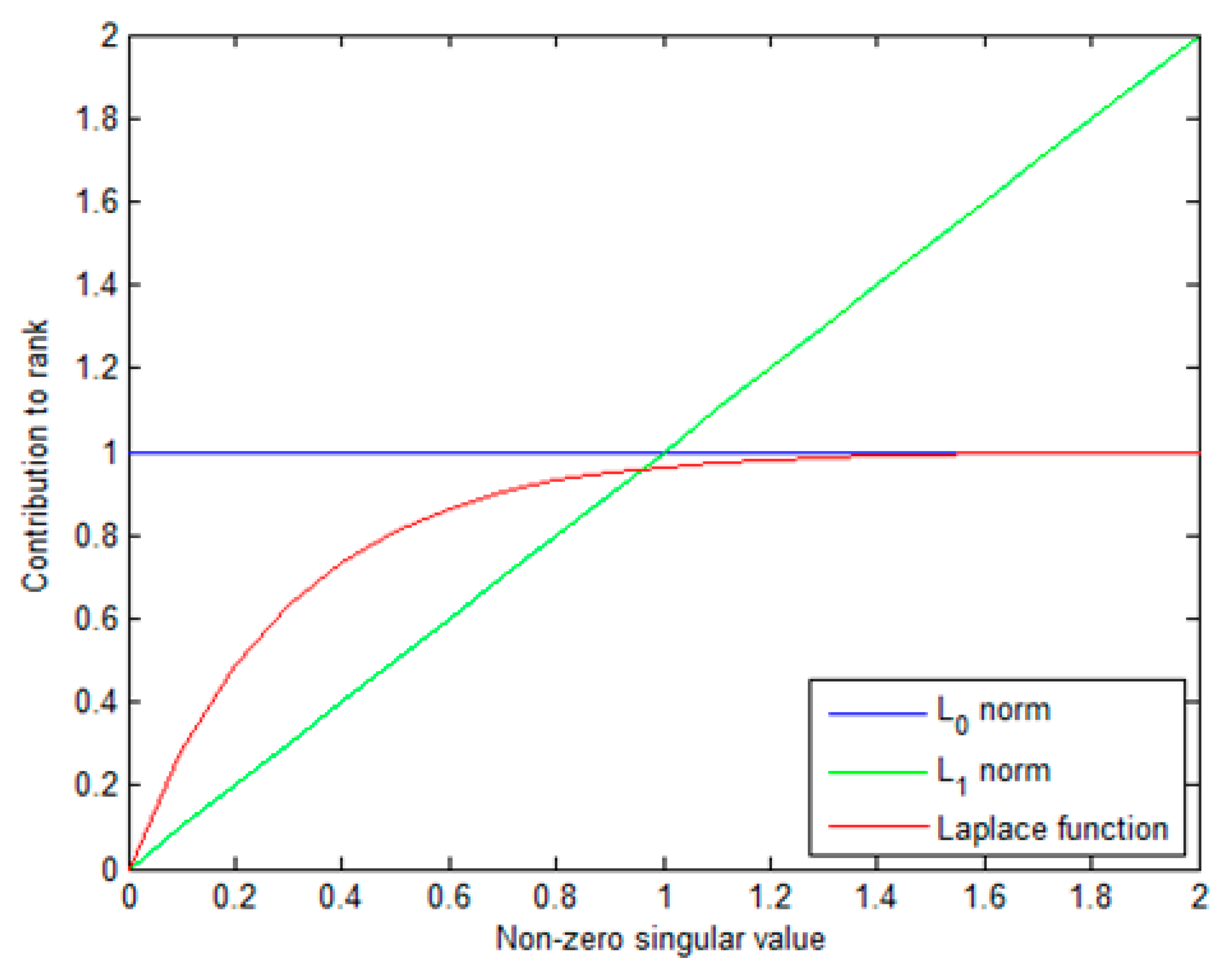
where $m=\min (m_1,m_2)$ and $\epsilon$ is a positive constant. $\varphi (x)=1-e^{-x/\epsilon }$ represents a Laplace function, which can approximate to the ${\ell }_0$-norm better compared with ${\ell }_1$-norm, as shown in Figure 3. Moreover, different from PSTNN, the Laplace function can automatically distribute the appropriate weight to each singular value. Therefore, the sum of the Laplace function is a better surrogate for tensor multi-rank.

The Laplace function based non-convex tensor rank surrogate has some useful properties [45]. Firstly, $\underset{\epsilon \to 0}{\lim }{\Vert \mathcal{X}\Vert }_{\epsilon }={\displaystyle {\sum }_{k=1}^{m_3}rank({\overline{\mathcal{X}}}^{(k)})}$, which means the rank approximately equal to the sum of all elements of multi rank, when $\epsilon$ is a small value. Secondly, ${\Vert \mathcal{U}\mathcal{X}\mathcal{V}\Vert }_{\epsilon }={\Vert \mathcal{X}\Vert }_{\epsilon }$, for any orthonormal tensor $\mathcal{U}\in {ℝ}^{m_1\times m_1\times m_3}$ and $\mathcal{V}\in {ℝ}^{m_2\times m_2\times m_3}$. Thirdly, ${\Vert \mathcal{X}\Vert }_{\epsilon }\ge 0$ for any $\mathcal{X}\in {ℝ}^{m_1\times m_2\times m_3}$, and ${\Vert \mathcal{X}\Vert }_{\epsilon }=0$ if and only if $\mathcal{X}=0$.

Based on the above considerations, the Laplace function based non-convex surrogate is an excellent candidate to represent the rank of a third-order tensor. Thus, we can minimize the non-convex surrogate to measure the low rank property of background patch-tensor $ℬ\in {ℝ}^{m_1\times m_1\times m_3}$. Aiming for the non-convex surrogate, optimization problem of the low rank tensor $ℬ$ is written in Equation (16)

$$\underset{ℬ}{\arg \min }{\Vert ℬ\Vert }_{\epsilon }+\frac{\gamma }{2}{\Vert ℬ-\mathcal{Z}\Vert }_F^2$$

(16)

From Equation (15), we can observe that the non-convex tensor rank surrogate is a linear combination of all frontal slices Laplace function in Fourier domain along the tube dimension. Therefore, in the Fourier domain, the optimization problem in Equation (16) can be achieved by solving $m_3$ matrix optimization problem [45], which is formulated as follows:

$$\underset{{\overline{ℬ}}^{(k)}}{\arg \min }{\displaystyle \sum _{j=1}^m\varphi ({\sigma }_j({\overline{ℬ}}^{(k)}))}+\frac{\gamma }{2}{\Vert {\overline{ℬ}}^{(k)}-{\overline{\mathcal{Z}}}^{(k)}\Vert }_F^2$$

(17)

where $k=1,\cdots ,m_3$, and ${\overline{\mathcal{Z}}}^{(k)},{\overline{ℬ}}^{(k)}\in {ℂ}^{m_1\times m_2}$. Given $\mathcal{Z}=\mathcal{U}\ast \mathcal{S}\ast {\mathcal{V}}^H$, Equation (17) is solved via the generalized weighted singular value thresholding operator [61], shown in Equations (18) and (19).

$${\overline{\mathcal{D}}}_{\frac{\nabla \varphi }{\beta }}^{(k)}(j,j)={({\overline{\mathcal{S}}}^{(k)}(j,j)-\frac{\nabla \varphi ({\sigma }_j^{k,l})}{\beta })}_{+}$$

(18)

$${\overline{ℬ}}^{(k)}={\overline{\mathcal{U}}}^{(k)}\ast {\overline{\mathcal{D}}}_{\frac{\nabla \varphi }{\beta }}^{(k)}\ast {\overline{\mathcal{V}}}^{(k)H}$$

(19)

where $\nabla \varphi ({\sigma }_j^{k,l})=\frac{1}{\epsilon }\exp (-\frac{{\sigma }_j^{k,l}}{\epsilon })$ is the gradient of $\varphi$ at ${\sigma }_j^{k,l}$, and ${\sigma }_j^{k,l}$ is the jth singular value of the kth frontal slice of $\overline{ℬ}$ at the lth iteration. Finally, $ℬ$ can be obtained by inverse FFT. Each iteration solution of the optimization problem in Equation (16) is briefly described in Algorithm 2.

Algorithm 2 Each iteration solution of optimization problem in Equation (16).

Input:${\overline{ℬ}}^l$, $\mathcal{Z}$, $\gamma$, $\epsilon$;

Output:${\overline{ℬ}}^{l+1}$,${ℬ}^{l+1}$;

1. Compute $\overline{\mathcal{Z}}=fft(\mathcal{Z},[],3)$;

2. Compute each frontal slice of ${\overline{ℬ}}^{l+1}$ by

for$k=1,\cdots ,\lceil (m_3+1)/2\rceil$do

1: $[{\overline{\mathcal{U}}}^{(k)},{\overline{\mathcal{S}}}^{(k)},{\overline{\mathcal{V}}}^{(k)}]=\mathrm{SVD}({\overline{\mathcal{Z}}}^{(k)})$;

2: ${\overline{\mathcal{D}}}_{\frac{\nabla \varphi }{\gamma }}^k$ can be obtained by Equation (18);

3: ${({\overline{ℬ}}^{l+1})}^{(k)}={\overline{\mathcal{U}}}^k\ast {\overline{\mathcal{D}}}_{\frac{\nabla \varphi }{\gamma }}^k\ast {\overline{\mathcal{V}}}^{(k)H}$;

end for

for $k=\lceil (m_3+1)/2\rceil ,\cdots ,1$ do

${({\overline{ℬ}}^{l+1})}^{(k)}=conj({({\overline{ℬ}}^{l+1})}^{(m_3-k+2)})$;

end for

3. Compute${ℬ}^{l+1}=ifft({\overline{ℬ}}^{l+1},[],3)$;

3.2. Local Prior Weight Map

It has been observed that local prior is different from nonlocal prior, and that local prior is a significant supplement to IPT detection framework [23]. In the RIPT model, the local structure map is used as local prior information to weight the target patch-tensor. The PSTNN model further analyzes the local structure of the infrared image and proposes an improved local structure weight map. Actually, the background should be suppressed and the target should be enhanced as much as possible in the local prior weight map. A saliency map based on local contrast has similar effect. Thus, we can construct the local prior weight map by utilizing local contrast features.

In infrared small target detection community, the concept of local contrast has been extensively applied [33,34]. Considering that the small target is brighter than its adjacent background in the local region, Xia et al. [9] proposed a local contrast element to describe the discontinuity between target and local adjacent background.

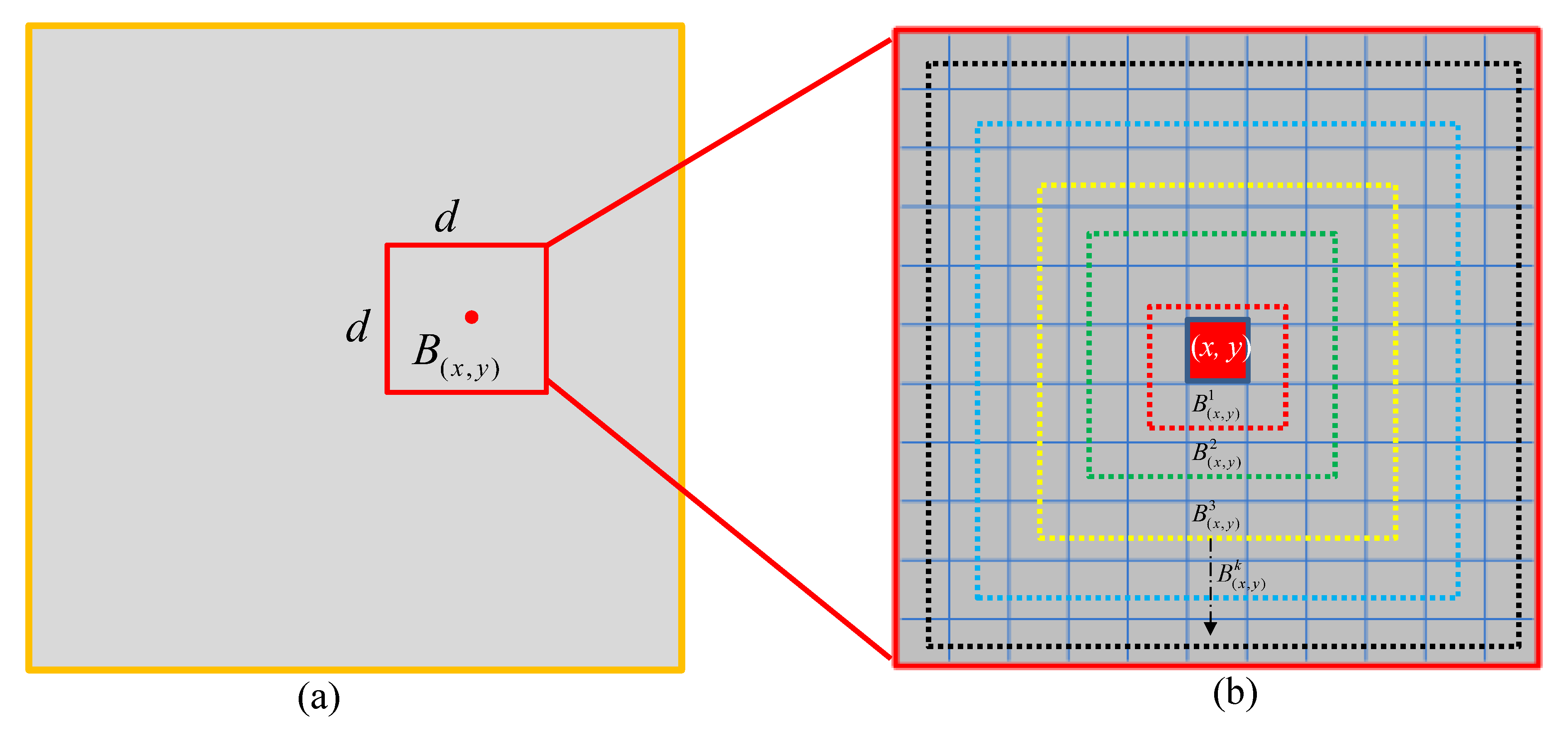
For the infrared image $f_D$, sub-block $B$ is defined as a local region in the whole image. In Figure 4a, a sub-block $B_{(x,y)}$ of size $d\times d$ is shown, $(x,y)$ denotes the center pixel location of the sub-block. $B_{(x,y)}^k$ represents a set of all neighborhood pixels, the Chebyshev distance of which to the center location $(x,y)$ is $k$, and is defined as follows:

$$B_{(x,y)}^k=\{(i,j)|\max (\left|i-x\right|,\left|j-y\right|)=k\}$$

(20)

The construction of $B_{(x,y)}^k$ is shown in Figure 4b; the $B_{(x,y)}^k$ corresponding to different $k$ values is represented by dotted lines with different colors. Defining $(i_{xy}^k,j_{xy}^k)$ as the pixel in $B_{(x,y)}^k$ that has the minimum difference with the center pixel, we have

$$(i_{xy}^k,j_{xy}^k)=\underset{(i,j)\in B_{(x,y)}^k}{\arg \min }\left|f(x,y)-f(i,j)\right|,\forall k\in \{1,\cdots ,\lfloor d/2\rfloor \}$$

(21)

where $f(i,j)$ and $f(x,y)$ are the grayscale of the corresponding pixels and $\lfloor \cdot \rfloor$ is the floor function. Then, a local contrast element $c_{xy}^k$ can be formulated as

$$c_{xy}^k=f(x,y)-f(i_{xy}^k,j_{xy}^k),\forall k\in \{1,\cdots ,\lfloor d/2\rfloor \}$$

(22)

Using the minimal operation in Equation (21), the local contrast element is sensitive to the direction information. That is because the small infrared target generally obeys the Gaussian distribution of spot-like; in other words, its information is similar in all directions, while the background edge commonly has a specific direction in the sub-block and the information varies greatly in different directions. As a result, local contrast element can effectively distinguish the small target and the salient clutter edges, such as cloud edge, building edge. By utilizing the local contrast element, a local energy feature which describes the discontinuity structure between a center pixel and its neighboring pixels can be defined as

$$LE(x,y)={\displaystyle \sum _{k=1}^{\lfloor d/2\rfloor }{c}_{xy}^k}$$

(23)

Considering for practical applications, the infrared small target shows a patch brighter than the surrounding background. Thus, pixels with contrast energy below 0 are considered as dark spots and should be excluded, and the saliency map $SM$ can be obtained by Equation (24):

$$SM(x,y)=\{\begin{array}{ll}LE(x,y)& LE(x,y)>0\\ 0& \mathrm{otherwise}\end{array}$$

(24)

Further, the local prior weight map $W_{lp}$ is defined as normalization of $SM$:

$$W_{lp}=\frac{SM-s{m}_{\min }}{s{m}_{\max }-s{m}_{\min }}$$

(25)

where $s{m}_{\max }$ and $s{m}_{\min }$ denote the maximum and minimum of $SM$. The different local prior weight maps are displayed in Figure 5. By using the local energy feature, it can be observed that the complex background clutters are fairly suppressed and the target is effectively enhanced in the proposed local prior weight map. Compared with the prior weight map of PSTNN, the proposed local energy feature can suppress the strong edge more significantly.

Finally, using the approach of the tensor construction in Figure 2, the prior weight map $W_{lp}$ can be converted into a tensor form, $W_{lp}$.

3.3. Structured Sparse Regularization

In the process of background–target separation, some rare structures tend to enter the sparse target component. One of the challenges of almost all approaches based on patch image models is rare structure effect [32]. Since many objects have a streamlined appearance in real scenes [62], we can consider that most of rare structures, such as the stubborn edges, remaining in the target image are linear structural sparse relative to the whole data of an input image [42]. Therefore, to minimize these rare structures being transferred to sparse target component, we introduce an extra tube-wise sparse tensor regularization term utilizing ${\ell }_{1,1,2}$-norm to IPT model [50]. The ${\ell }_{1,1,2}$-norm of third-order tensor is similar to ${\ell }_{2,1}$-norm of matrix which has the ability to identify the sample outlier, while most outliers can be associated with sparse structure [32,42]. Then, an input infrared patch-tensor $\mathcal{D}$ can be decomposed into three components, which are sparse target tensor $\mathcal{T}$, low-rank background tensor $\mathcal{B}$, and structured sparse edge tensor $\mathcal{S}$, respectively, as follows:

$$\mathcal{D}=ℬ+\mathcal{T}+\mathcal{S}$$

(26)

where the ${\ell }_{1,1,2}$-norm of $\mathcal{S}$ is denoted as ${\Vert \mathcal{S}\Vert }_{1,1,2}$, which can be defined as ${{\displaystyle {\sum }_{i,j}\Vert \mathcal{S}(i,j,:)\Vert }}_2$.

3.4. The Proposed NTRS Model

According to the above description, a target detection model utilizing the non-convex tensor rank surrogate, the local contrast energy, and the structured sparse regularization, which is named NTRS, is formulated as follows:

$$\begin{array}{c}\underset{\mathcal{B},\mathcal{T},\mathcal{S}}{\min }{\Vert \mathcal{B}\Vert }_{\epsilon }+\lambda {\Vert \mathcal{W}\odot \mathcal{T}\Vert }_0+\beta {\Vert \mathcal{S}\Vert }_{1,1,2}\\ s.t.\mathcal{D}=\mathcal{B}+\mathcal{T}+\mathcal{S}\end{array}$$

(27)

where $\odot$ denotes the Hadamard product; ${\mathcal{W}}_{rec}$ is the tensor, each element of which is the reciprocal of the corresponding element in ${\mathcal{W}}_{lp}$; and $\lambda$ and $\beta$ are positive trade-off coefficients.

Due to the non-convex and non-smooth of ${\ell }_0$-norm, it is difficult to directly solve problems involving that norm. For tractable computation, we characterize the sparsity of the target tensor by employing ${\ell }_1$-norm as other many detection models. A reweighted ${\ell }_1$-norm minimization is proposed to enhance sparsity in [63]. After that, the reweighted scheme, which can speed up the convergence rate and alleviate the imbalance that the larger numerical value suffers the greater penalty than the smaller one [8], is widely studied and applied [64,65,66]. Thus, the reweighted scheme is utilized in this paper, too. Moreover, the gray values of the real small targets are usually greater than those of non-target sparse spots. Thus, the sparse reweight can be given as follows:

$${\mathcal{W}}_{sw}^l=\frac{c}{\left|{\mathcal{T}}^l\right|+\eta }$$

(28)

where $c$ is a non-negative constant, and can be set to 1 for simplicity [23,32]. To prevent division by zero, $\eta$ represents a tiny positive constant and is set to ${10}^{-8}$ in this paper. $l$ stands for the lth iteration. The local prior weight and the sparse reweight can be combined to get the final weight tensor, as follows:

$$\mathcal{W}={\mathcal{W}}_{rec}\odot {\mathcal{W}}_{sw}$$

(29)

Finally, the proposed NTRS model (Equation (27)) is rewritten as:

$$\begin{array}{c}\underset{\mathcal{B},\mathcal{T},\mathcal{S}}{\min }{\Vert \mathcal{B}\Vert }_{\epsilon }+\lambda {\Vert \mathcal{W}\odot \mathcal{T}\Vert }_1+\beta {\Vert \mathcal{S}\Vert }_{1,1,2}\\ s.t.\hspace{1em}\mathcal{D}=\mathcal{B}+\mathcal{T}+\mathcal{S}\end{array}$$

(30)

3.5. Solution of NTRS Model

In this subsection, an optimization algorithm based on ADMM [67], which has high precision and fast convergence speed, is proposed to solve Equation (30). The augmented Lagrangian function of that can be defined as

$$\mathcal{L}(\mathcal{B},\mathcal{T},\mathcal{S},\mathcal{Y},\mu )={\Vert \mathcal{B}\Vert }_{\epsilon }+\lambda {\Vert \mathcal{W}\odot \mathcal{T}\Vert }_1+\beta {\Vert \mathcal{S}\Vert }_{1,1,2}+\langle \mathcal{Y},\mathcal{B}+\mathcal{T}+\mathcal{S}-\mathcal{D}\rangle +\frac{\mu }{2}{\Vert \mathcal{B}+\mathcal{T}+\mathcal{S}-\mathcal{D}\Vert }_F^2$$

(31)

where $\mathcal{Y}$ and $\mu >0$ are the Lagrange multiplier and the penalty factor, respectively. $\langle \cdot \rangle$ is the two third-order tensors inner product.

Subsequently, ADMM decomposes minimization of $ℒ$ into several subproblems, and $ℬ$, $\mathcal{T}$, $\mathcal{S}$ can be updated by an iterative approach. Specifically, at the $(l+1)$th iteration, ${ℬ}^{l+1}$, ${\mathcal{T}}^{l+1}$, and ${\mathcal{S}}^{l+1}$ are obtained via solving the three subproblems, as follows:

$${\mathcal{B}}^{l+1}=\arg \min {\Vert \mathcal{B}\Vert }_{\epsilon }+\frac{{\mu }^l}{2}{\Vert \mathcal{B}+{\mathcal{S}}^l+{\mathcal{T}}^l-\mathcal{D}+\frac{{\mathcal{Y}}^l}{{\mu }^l}\Vert }_F^2$$

(32)

$${\mathcal{T}}^{l+1}=\arg \min \lambda {\Vert \mathcal{T}\odot \mathcal{W}\Vert }_1+\frac{{\mu }^l}{2}{\Vert {\mathcal{B}}^{l+1}+{\mathcal{S}}^l+\mathcal{T}-\mathcal{D}+\frac{{\mathcal{Y}}^l}{{\mu }^l}\Vert }_F^2$$

(33)

$${\mathcal{S}}^{l+1}=\arg \min \beta {\Vert \mathcal{S}\Vert }_{1,1,2}+\frac{{\mu }^l}{2}{\Vert {\mathcal{B}}^{l+1}+\mathcal{S}+{\mathcal{T}}^{l+1}-\mathcal{D}+\frac{{\mathcal{Y}}^l}{{\mu }^l}\Vert }_F^2$$

(34)

where $\mathcal{Y}$ and $\mu$ can be updated by the Equations (35) and (36), respectively.

$${\mathcal{Y}}^{l+1}={\mathcal{Y}}^l+{\mu }^l({\mathcal{B}}^{l+1}+{\mathcal{S}}^{l+1}+{\mathcal{T}}^{l+1}-\mathcal{D})$$

(35)

$${\mu }^{l+1}=\rho {\mu }^l$$

(36)

where $\rho >1$ is a constant. Let $\gamma ={\mu }^l$, $\mathcal{Z}=\mathcal{D}-{\mathcal{T}}^l-{\mathcal{S}}^l-\frac{{\mathcal{Y}}^l}{{\mu }^l}$, the subproblem in Equation (32) can be solved by Algorithm 2 of Section 3.1. For the subproblem in Equation (33), ${\mathcal{T}}^{l+1}$ can be calculated via a soft-thresholding operator [68], as shown in Equations (37) and (38):

$$S_{\theta }(y)=sign(y)\ast \max (\left|y\right|-\theta ,0)$$

(37)

$${\mathcal{T}}^{l+1}=S_{\raisebox{1ex}{$\lambda {\mathcal{W}}^l$}\!\left/ \!\raisebox{-1ex}{${\mu }^l$}\right.}(\mathcal{D}-{\mathcal{S}}^l-{\mathcal{B}}^{l+1}-\frac{{\mathcal{Y}}^l}{{\mu }^l})$$

(38)

Let $Q=\mathcal{D}-{\mathcal{B}}^{l+1}-{\mathcal{T}}^{l+1}-\frac{{\mathcal{Y}}^l}{{\mu }^l}$, the solution of subproblem in Equation (34) is given by

$${\mathcal{S}}^{l+1}(:,:,m)={\left(1-\frac{\beta }{{\mu }^l{\Vert Q(:,:,m)\Vert }_2}\right)}_{+}Q(:,:,m)$$

(39)

where $m=1,\cdots ,m_3$.

The convergence speed of the proposed model is a dominant factor to computational time of the whole detection algorithm. Generally, the given threshold of reconstruction relative error is used as the stopping criterion for robust principle component analysis (RPCA) problem [69]. However, it has been observed that number of non-zero elements among the sparse target tensor barely change after a few iterations [8,23]. Therefore, besides the reconstruction relative error, we could count the number of non-zero elements of target tensor as the stopping condition, which can be defined as ${\Vert {\mathcal{T}}^l\Vert }_0={\Vert {\mathcal{T}}^{l+1}\Vert }_0$, to reduce the iteration number.

Finally, we summarize the whole optimization process of NTRS model as Algorithm 3.

Algorithm 3 ADMM for solving the proposed NTRS model.

Input: Original patch-image $\mathcal{D}$, ${\mathcal{W}}_{lp}$, $\lambda$, $\beta$;

Initialize:${ℬ}^0={\mathcal{T}}^0={\mathcal{S}}^0={\mathcal{Y}}^0=0$, ${\overline{ℬ}}^0$ = 0, ${\mathcal{W}}_{sw}=1$, ${\mathcal{W}}^0={\mathcal{W}}_{rec}\odot {\mathcal{W}}_{sw}$, ${\mu }^0=0.002$, $\rho =1.1$, $tol={10}^{-7}$, $c=1$, $l=0$;

While not converged do

1: Fix the others and update ${ℬ}^{l+1}$ by Algorithm 2;

2: Fix the others and update ${\mathcal{T}}^{l+1}$ by

${\mathcal{T}}^{l+1}=S_{\raisebox{1ex}{$\lambda {\mathcal{W}}^l$}\!\left/ \!\raisebox{-1ex}{${\mu }^l$}\right.}(\mathcal{D}-{\mathcal{S}}^l-{\mathcal{B}}^{l+1}-\frac{{\mathcal{Y}}^l}{{\mu }^l})$;

3: Update ${\mathcal{S}}^{l+1}$ via

${\mathcal{S}}^{l+1}(:,:,m)={\left(1-\frac{\beta }{{\mu }^l{\Vert Q(:,:,m)\Vert }_2}\right)}_{+}Q(:,:,m)$;

4: Update ${\mathcal{Y}}^{l+1}$ via

${\mathcal{Y}}^{l+1}={\mathcal{Y}}^l+{\mu }^l({\mathcal{B}}^{l+1}+{\mathcal{S}}^{l+1}+{\mathcal{T}}^{l+1}-\mathcal{D})$;

5: Update ${\mathcal{W}}^{l+1}$ by

${\mathcal{W}}_{sw}^{l+1}=\frac{c}{\left|{\mathcal{T}}^{l+1}\right|+\eta }$;

${\mathcal{W}}^{l+1}={\mathcal{W}}_{rec}\odot {\mathcal{W}}_{sw}^{l+1}$;

6: Update ${\mu }^{l+1}$ by

${\mu }^{l+1}=\rho {\mu }^l$;

7: Inspect the stop conditions

$\frac{{\Vert {\mathcal{B}}^{l+1}+{\mathcal{T}}^{l+1}+{\mathcal{S}}^{l+1}-\mathcal{D}\Vert }_F^2}{{\Vert \mathcal{D}\Vert }_F^2}<tol$ or ${\Vert {\mathcal{T}}^l\Vert }_0={\Vert {\mathcal{T}}^{l+1}\Vert }_0$;

8: Update $l$

$l=l+1$;

End while

Output:${ℬ}^l$, ${\mathcal{T}}^l$, ${\mathcal{S}}^l$

3.6. Target Detection

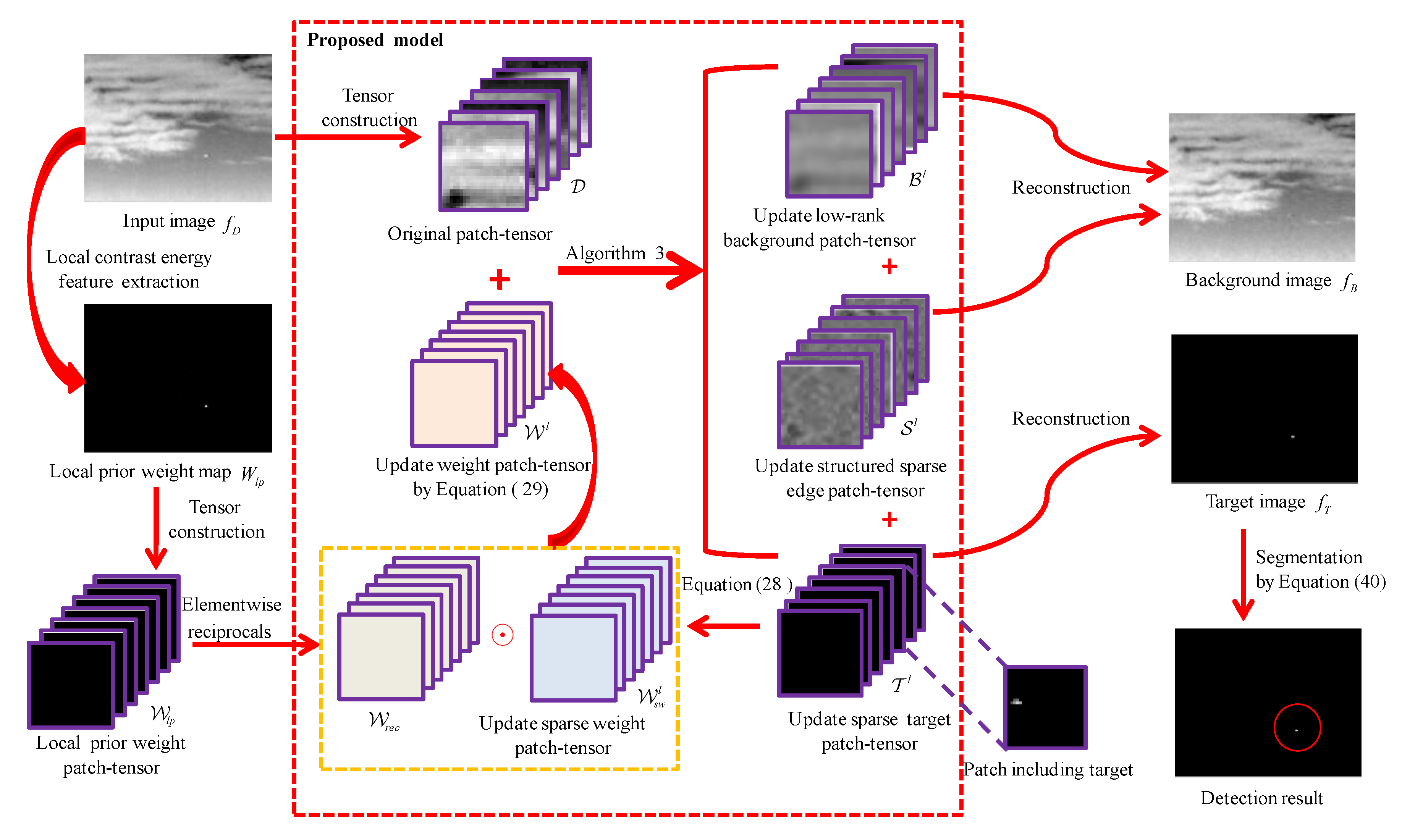
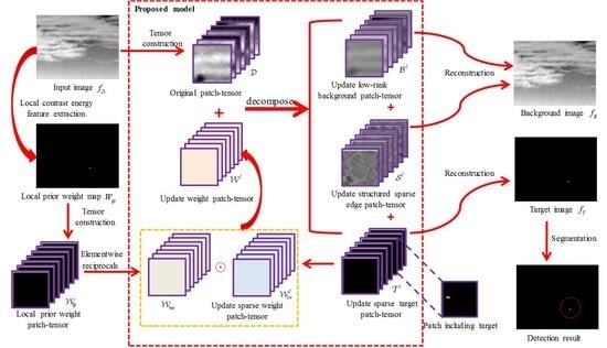
In Figure 6, we show the specific implementation procedure of the target detection method based on the proposed NTRS model. Meanwhile, the detailed steps are explained in the following.

(1)

Local prior map generation. For an input infrared image $f_D\in {ℝ}^{m\times n}$, its local prior weight map $W_{lp}\in {ℝ}^{m\times n}$ is calculated via Equation (25).

(2)

Patch-tensor construction. Original patch-tensor $\mathcal{D}\in {ℝ}^{m_1\times m_2\times m_3}$ can be constructed by stacking image patches which are obtained via sliding a window of size $m_1\times m_2$ over the input image, as shown in Figure 2. In the same way, the local prior weight patch-tensor ${\mathcal{W}}_{lp}\in {ℝ}^{m_1\times m_2\times m_3}$ can be constructed from local prior weight map.

(3)

Background–target–edge separation. By Algorithm 3, an original infrared patch-tensor $\mathcal{D}$ can be decomposed into three patch-tensor components: the low rank background $ℬ$, the sparse target $\mathcal{T}$, and the structured sparse edge $\mathcal{S}$.

(4)

Image reconstruction. The two-dimensional image can be reconstructed by the inverse operation of patch-tensor construction [42]. Considering that structured edges are also background, we first sum $ℬ$ and $\mathcal{S}$ as the final background patch-tensor $ℬ$. Then, the target image $f_T$ and the background image $f_B$ are reconstructed from target patch-tensor $\mathcal{T}$ and background patch-tensor $ℬ$, respectively. For the overlapped positions, one-dimensional median filter can be used to determine the values.

(5)

Target detection. Considering that the pixels of the true targets have higher grayscale in the reconstructed target image [70], small targets can be extracted via a simple adaptive threshold segmentation algorithm. The threshold $Th$ is as follows:

$$Th=f_{Tmean}+\rho \ast f_{Tstd}$$

(40)

where $f_{Tstd}$ and $f_{Tmean}$ are the standard deviation and mean of the reconstructed target image $f_T$, respectively. $\rho$ is an empirical coefficient to compromise false alarm rate and detection probability.

4. Experimental Results and Analysis

4.1. Experimental Preparation

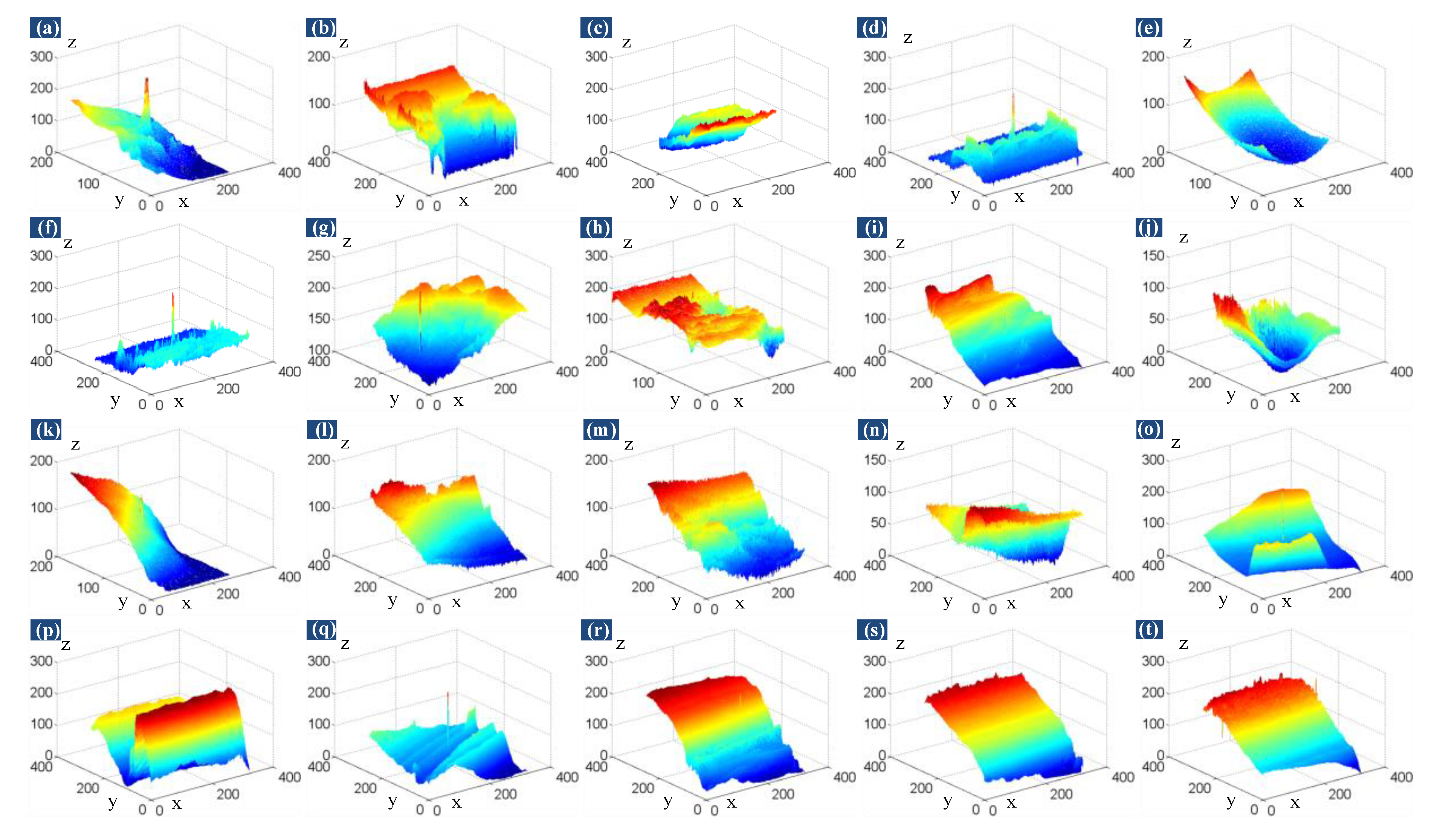
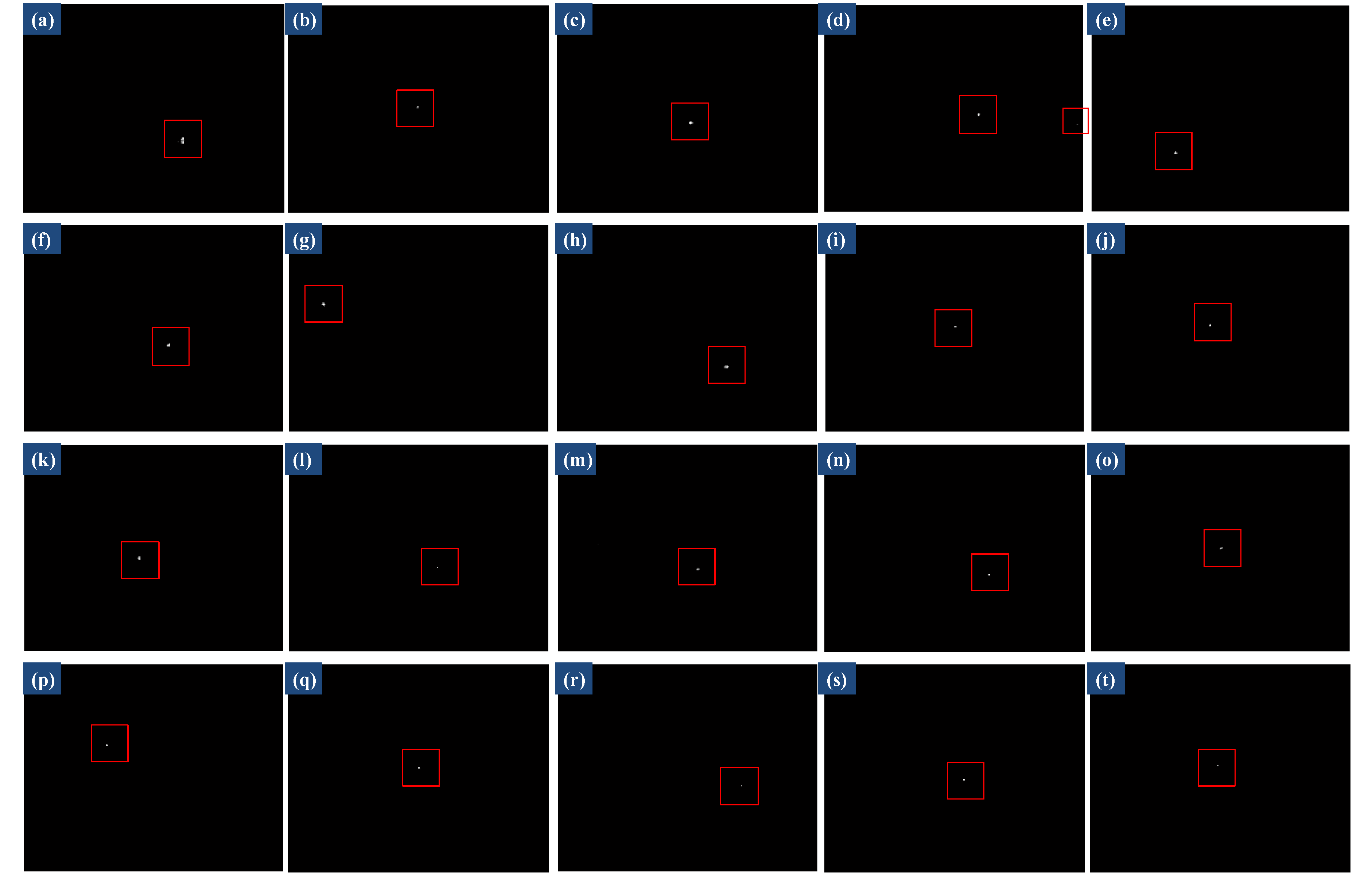
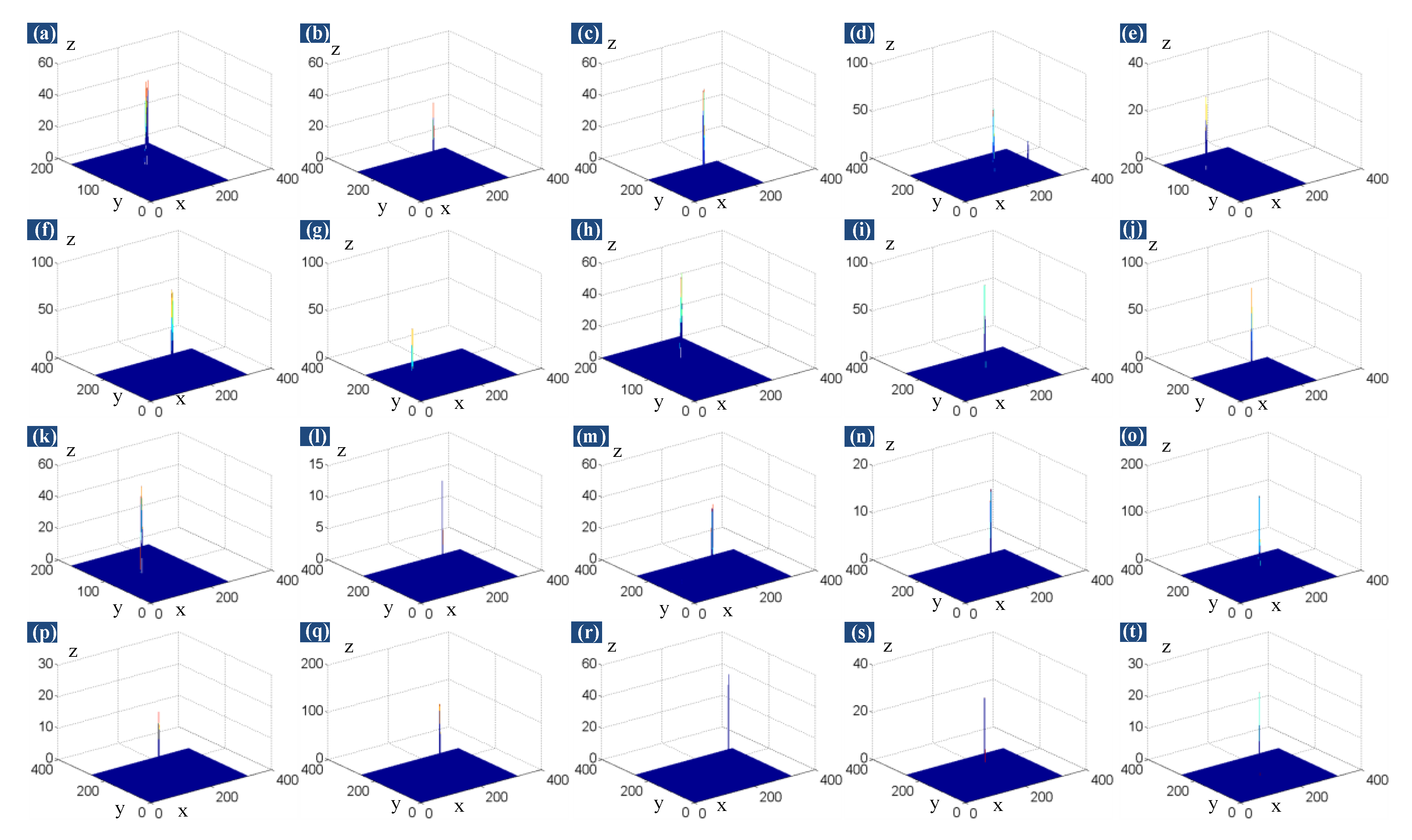
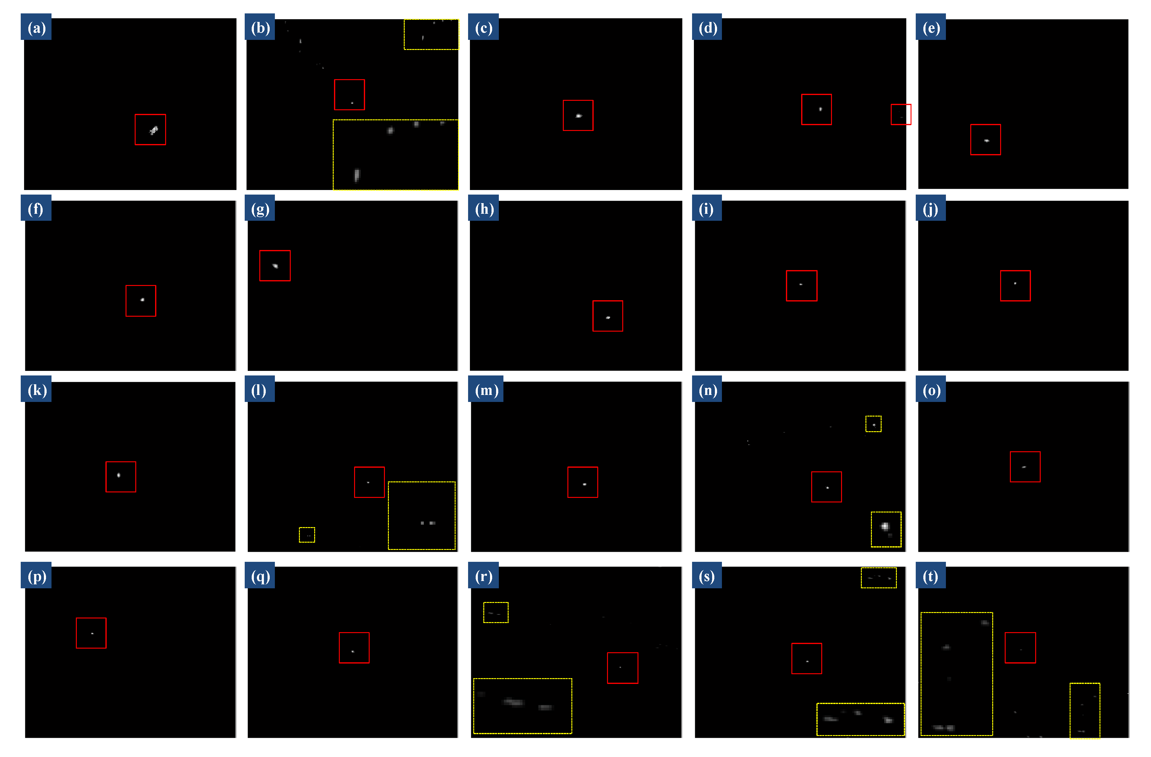
To demonstrate the effectiveness of our method in multiple aspects, such as robustness to noise and various background, the capability of small target enhancement and background suppression, detection performance, and computational time, extensive experiments were conducted. In our experiments, fourteen single frame infrared images of different scenes, varying from homogeneous background containing extreme faint small target to complicated background with prominent clutters and interferences, and six real sequences were utilized to verify our method. The fourteen single images (a–n) and the representative images (o–t) of the six real sequences, a total of twenty images with different scenes, are displayed in Figure 7. To facilitate visualization, these images were converted to the identical size and each real target is indicated by a red square box. Figure 8 shows the 3D mesh views corresponding to the images. The six real sequences were captured via an infrared thermal camera (Its infrared sensor is a long wave infrared focal plane arrays, MARS LW K508), which is mounted on aircraft to detect aerial targets and its imaging resolution is $320\times 256$. The dynamic range of the original image data is 14bit and we converted that to 8bit (0–255) by using linear mapping. All six sequences contain the complex background and clutter, such as different types of clouds and various ground highlight interferences. Meanwhile, all targets are small. Detailed descriptions are given in

Table 1. Detailed description of the six real sequences.

Sequence (Seq)	Length	Image Size	Target and Background Description
Sequence 1 (Scene o)	180	320 × 256	Target lies in flat area between two complex clouds, moving fast with changing shape, brightness
Sequence 2 (Scene p)	168	320 × 256	Target appears near the cloud edge, with very bright cloud and banded cloud, very dim tiny
Sequence 3 (Scene q)	191	320 × 256	Target is above the complex structure cloud, moving fast with changing size
Sequence 4 (Scene r)	210	320 × 256	Target is submerged in heavy cloud, with banded cloud, small size, low contrast
Sequence 5 (Scene s)	233	320 × 256	Background includes sky and ground, with heavy cloud, target with small size and low contrast
Sequence 6 (Scene t)	292	320 × 256	Target closes to ground, with a large number of ground highlight interferences, very dim

Notes: Scenes o–t, as shown in Figure 7o–t, are the representative frames of Sequence 1–6, respectively.

.

Six other classical and advanced methods, namely local contrast measure (LCM) [34], Top-hat filter [27], multi-scale patch contrast measure (MPCM) [10], RIPT model [23], IPI model [38], and PSTNN model [8] were used as the benchmarks for the overall comparison. The parameter settings of the seven approaches including ours are summarized in

Table 2. Detailed parameter settings for the seven methods.

Method	Parameters
Top-hat	Structure size: 5 × 5, shape: disk
LCM	Largest scale: $l_{\max }=3$, size of u: 3 × 3, 5 × 5, 7 × 7
MPCM	$L=3,$$N=5,7,9$
IPI	Sliding step: 10, patch size: 50 × 50, $\lambda =1/\sqrt{\min (m,n)}$, $\epsilon ={10}^{-7}$
RIPT	Sliding step: 10, patch size: 30 × 30, $\lambda =L/\sqrt{\min (m_1,m_2,m_3)}$, $L=1$, $h=1$, $\epsilon ={10}^{-7}$
PSTNN	Sliding step: 40, patch size: 40 × 40, $\lambda =0.6/\sqrt{\max (m_1,m_2)\ast m_3}$, $\epsilon ={10}^{-7}$
Ours	Sliding step: 30, patch size: 40 × 40, $\lambda =0.75/\sqrt{\max (m_1,m_2)\ast m_3}$, $\beta =10.5\ast \lambda$, $\mu =0.002$, $tol={10}^{-7}$

.

4.2. Evaluation Metrics

In this subsection, several commonly used performance evaluation metrics of infrared small target detection methods are introduced [3]. The signal-to-clutter ratio (SCR) is a basic indicator to measure the target saliency. It is also a measurement of the detection difficulty. Its formula is:

$$\mathrm{SCR}=\frac{\left|{\overline{\mu }}_t-{\overline{\mu }}_b\right|}{{\sigma }_b}$$

(41)

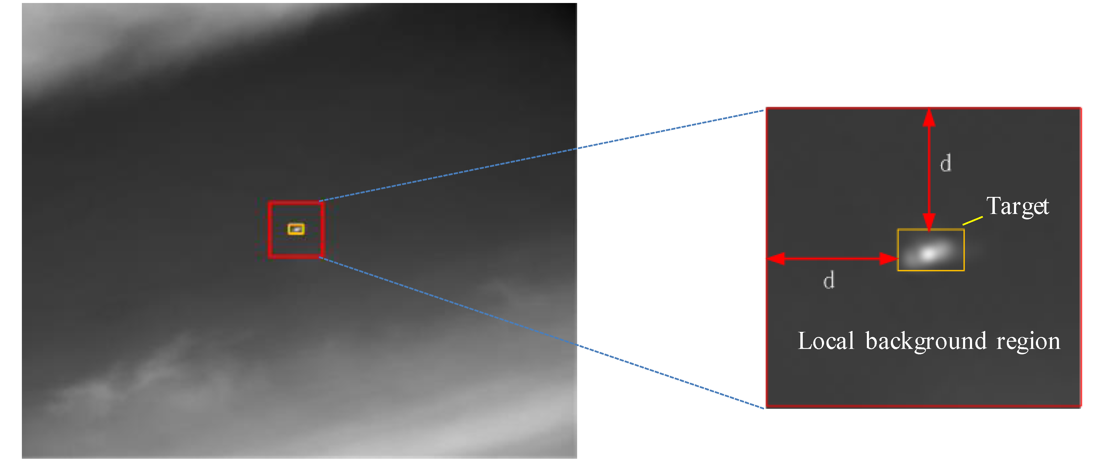
where SCR is calculated in local adjacent region of the target, as shown in Figure 9. ${\overline{\mu }}_t$ and ${\overline{\mu }}_b$ denote the gray mean values of the target region and the neighborhood background region surrounding the target, respectively. ${\sigma }_b$ is the standard deviation of the target adjacent background. We set $d=25$ in our experiments. Generally, when the SCR is higher, the detection will be easier. Based on SCR, the gain of SCR (GSCR), which is the most frequently adopted criterion, can be defined:

$$\mathrm{GSCR}=\frac{{\mathrm{SCR}}_{out}}{{\mathrm{SCR}}_{in}}$$

(42)

where ${\mathrm{SCR}}_{out}$ and ${\mathrm{SCR}}_{in}$ denote the SCR of the processed image (which is the reconstructed target image for the proposed method in this paper) and the original image, respectively. Higher GSCR means greater ability of target enhancement.

Background suppression factor (BSF) is another typical evaluation metric, which reflects the ability of background suppression of detection methods. Higher BSF means that the detection algorithm can suppress background clutter more effectively. BSF is defined as

$$\mathrm{BSF}=\frac{{\sigma }_{in}}{{\sigma }_{out}}$$

(43)

where ${\sigma }_{out}$ and ${\sigma }_{in}$ stand for the corresponding standard deviation values of the local background in the processed image and the original image, respectively.

In addition to the target enhancement and background suppression ability indicator, false positive rate (FPR) and true positive rate (TPR), which represent false alarm rate and detection probability, respectively, were utilized to evaluate comprehensive target detection ability of several methods. FPR and TPR are formulated as follows:

$$\mathrm{FPR}=\frac{\mathrm{number}\mathrm{of}\mathrm{nontarget}\mathrm{pixels}\mathrm{detected}}{\mathrm{total}\mathrm{number}\mathrm{of}\mathrm{pixels}\mathrm{in}\mathrm{all}\mathrm{images}}$$

(44)

$$\mathrm{TPR}=\frac{\mathrm{number}\mathrm{of}\mathrm{true}\mathrm{targets}\mathrm{detected}}{\mathrm{number}\mathrm{of}\mathrm{true}\mathrm{targets}}$$

(45)

Usually, the value of FPR is very small. Receive operating characteristic (ROC) curve can be drawn according to TPR and FPR, and then the area under curve (AUC) can be obtained. The ROC curve reveals the trade-off between the false-alarm rate and detection probability: the closer the curve is to the left upper corner, the more robust is the target detection ability. In the same way, the AUC value increases with improving performance of the detection approach.

4.3. Parameter Analysis

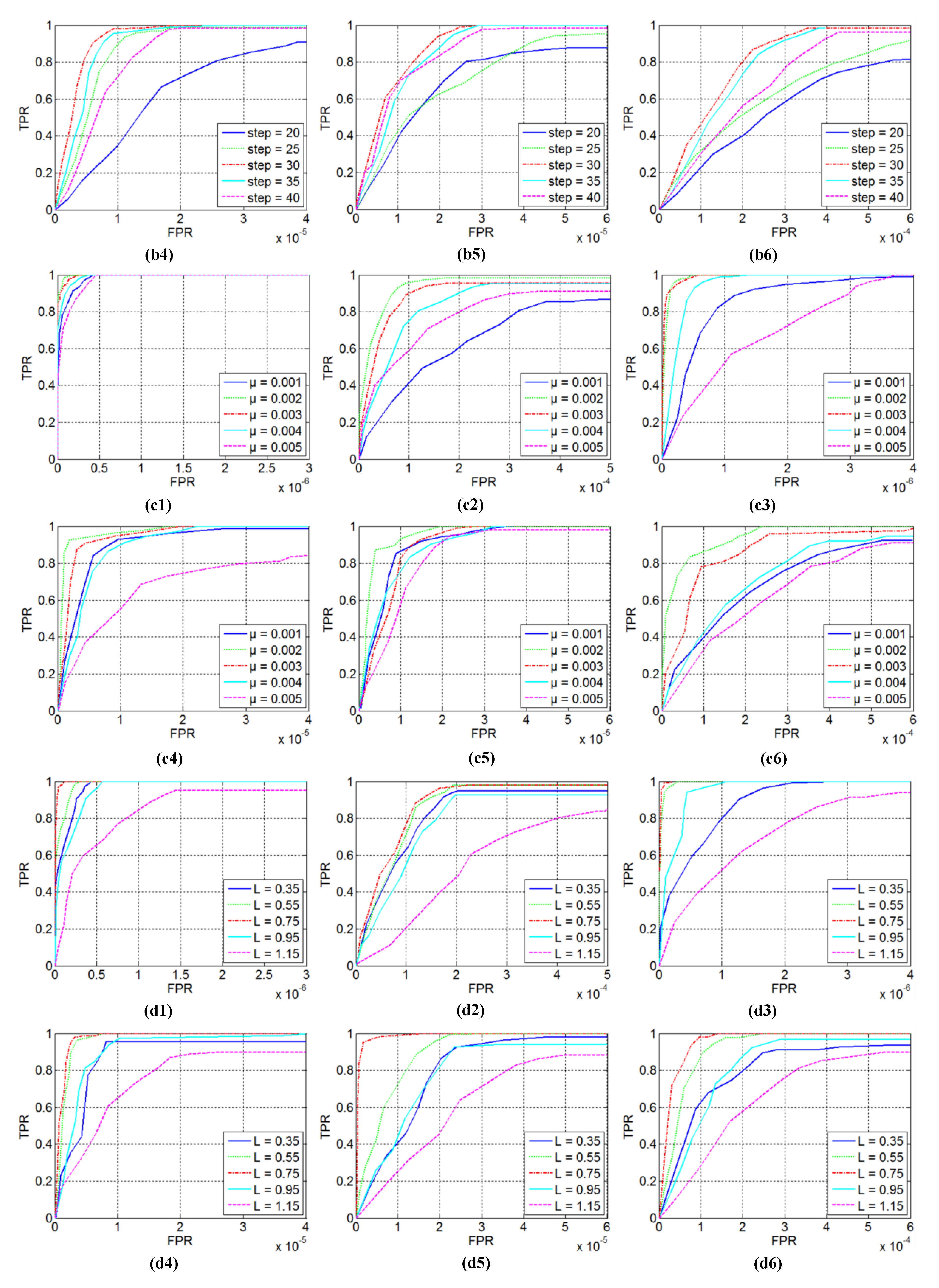
Several key parameters are included in the proposed NTRS model, for instance sliding step, patch size, compromising parameters $\lambda$ and $\beta$, and penalty factor $\mu$. These parameters would affect detection ability and robustness of the model under different backgrounds. Thus, to achieve excellent performance in most cases, especially for real scenes, it is necessary to select appropriate parameter setting. We selected the parameter values through experiments and analyzed them in detail. In the experiments, other parameters were fixed while one was tuned. In Figure 10, we show the ROC curves of different parameters on six tested infrared sequences (Sequences 1–6).

4.3.1. Patch Size

Patch size not only has the critical influence on detection performance, but also affects computational time of the algorithm [8]. On the one hand, it is obvious that a smaller patch size could result in a lower computational complexity of NTRS model; however, it would weaken the sparsity of the target. On the other hand, a larger patch size is usually adopted to ensure that the target is sufficiently sparse to deal with the changing size target, but it would reduce the correlation between patches and relax the sparsity of patch too much, resulting in some clutter with sparse characteristics. To investigate the influence of patch size on the proposed model, the patch size was varied from 20 to 60 by taking 10 as a length of stride. The ROC curves on six tested sequences are shown in Figure 10a1–a6. From these ROC curves, we can observe that the detection performance of the patch size within 30–50 is generally acceptable and that the model achieves the best performance on the all sequences when 40 is set for the patch size. It is also observed that the detection performance decreases when the patch size is 20 or 60; especially, when the patch size is 60, the detection results are the worst. These demonstrate our previous analysis that both overlarge and too small patch size would result in low detection performance. Hence, we set the patch size to 40 in the experiment.

4.3.2. Sliding Step

The sliding step determines the number of frontal slices that we can obtain for constructing patch-tensor. Similar to the patch size, it would influence the detection performance and computation time simultaneously. A larger sliding step means there would be fewer frontal slices, which would reduce the operation time of Algorithm 1. However, a larger sliding step may degrade the redundancy of the original patch-tensor and undermine the nonlocal correlation of the background [17], which weakens the background clutter separation ability of the proposed model. On the contrary, a smaller sliding step would increase computation time of the model and weaken the sparsity of the target due to more frontal slices containing the target. In addition, the sliding step should not be larger than the patch size to avoid missing the target. To inquire into influence of the sliding step, we changed it from 20 to 40 with five intervals. Corresponding ROC curves for the six sequences are displayed in Figure 10b1–b6. Analyzing the ROC curves, we can conclude that the proposed model is robust to the variation of sliding step between 25 and 40. At the same time, we observe that, when the sliding step is set to 30, the proposed model achieves the optimal detection performance on all sequences. Thus, 30 is the best choice for the sliding step.

4.3.3. Penalty Factor $\mu$

Penalty factor $\mu$ plays an important role in the optimization process of the model and controls the compromise between the sparse component and low-rank component. On the one hand, a smaller $\mu$ would preserve more details in the low-rank component and prevent more non-target interference from entering the sparse component. As a result, less background clutter remains in the target patch-tensor. However, details of the target may also be kept in the low-rank component, so that the small target suffers from over-shrinking or even is missed. On the other hand, the target details can be preserved by a larger; nevertheless, this may lead to more background clutter appearing in the target patch-tensor. For the best detection performance, it is necessary to select a suitable value of $\mu$ to keep a reasonable tradeoff between false-alarm rate and detection probability. Therefore, we varied the penalty factor $\mu$ from 0.001 to 0.005 with a step of 0.001. The ROC curves for the six tested sequences are shown in Figure 10c1–c6. It can be observed that the optimal detection performance is obtained in most instances when $\mu =0.002$. A larger or smaller value is not an optimal choice. Therefore, we used 0.002 as the best penalty factor value for our experiments.

4.3.4. Compromising Parameters $\lambda$ and $\beta$

In NTRS model, the parameters $\lambda$ and $\beta$ regulate the compromise among sparse target tensor, structured sparse edge tensor and low-rank background tensor. It is necessary to fine tune them. Although a large $\lambda$ value would lead to the purer target image, small targets might be over-shrunk. In contrast, a small $\lambda$ value can preserve more details of the target. However, background residuals would be kept in target image. Considering $\lambda$ and $\beta$ are used to constrain sparse (or structured sparse) components, they have similar characteristics. For simplicity, we first made $\beta =k\ast \lambda$ and empirically chose $k=10.5$. Next, to investigate the influence of $\lambda$ on detection performance, similar to PSTNN model, we let $\lambda =L/\sqrt{\max (m_1,m_2)\ast m_3}$ and varied $L$ from 0.35 to 1.15 with an interval of 0.15 instead of varying $\lambda$ directly. ROC curves for the six tested sequences are illustrated in Figure 11d1–d6. From the illustrations, it can be observed that the detection result is relatively poor when L is too larger ($L=1.15$) or too small ($L=0.35$). Especially, when $L=1.15$, we obtain the worst performance with some targets always being missed in each sequence. Meanwhile, the detection results show that the best performance is achieved for all sequences when $L=0.75$. Thus, we used $\lambda =0.75/\sqrt{\max (m_1,m_2)\ast m_3}$ in the following experiments.

4.4. Qualitative Evaluation

4.4.1. Robustness to Various Scenes

Wide adaptability to various scenes is a crucial ability for target detection algorithm. Here, the various scenes mean three points: the diversity of background, the variability of target and uncertainty of target position in background. Infrared backgrounds are diverse, from uniform background to complex background, from sky background with cloud to sea or ground background, and so on. Because of the changing distance from the target to the imaging sensor, the target size in the image is variable, from one pixel to dozens of pixels. Meanwhile, the brightness of the target in the image may also vary dramatically. Furthermore, the target may appear in different positions of the background. For example, to the sky background with cloud, small target may be above the cloud, in the cloud, or near the cloud edge. The twenty single frame images, which are shown in Figure 7, cover most of the above-mentioned cases and are very representative. Therefore, these images can be used to test the proposed method’s robustness.

In Figure 11, we show the target images reconstructed by the proposed method for the twenty different scenes in Figure 7. Corresponding 3D mesh views of the reconstructed target images are shown in Figure 12. Figure 11 shows that the various types of background clutters are completely wiped out and desired targets are well preserved. Figure 12 shows that each small target is transformed into the most prominent spot of the 3D mesh view. Comparing Figure 8 and Figure 12 (3D mesh views of original images), we can see more clearly that all the small targets have been enhanced markedly by the proposed approach. Meanwhile, various background clutters are effectively suppressed. We also show the target images processed by PSTNN model, which is the most advanced method for small infrared target detection in Figure 13. From the processed results, although PSTNN can detect all targets, some background clutters (marked by yellow square boxes) are still retained in the processed target images. Therefore, we conclude that our method can handle different targets and backgrounds, and is quite robust to various scenes.

4.4.2. Anti-Noise Performance

In practical application, an infrared image is inevitably contaminated by various noises [1]. Thus, in addition to robustness for various scenes, anti-noise ability is another important indicator for infrared small detection method. The anti-noise performance of our model was evaluated via an experiment.

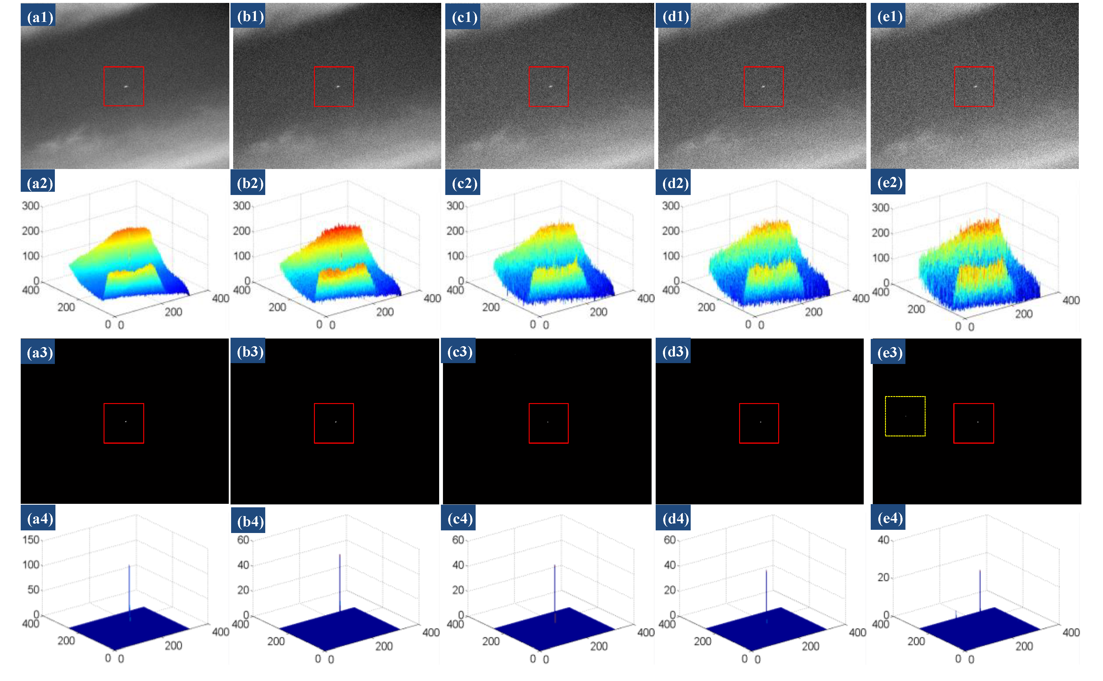
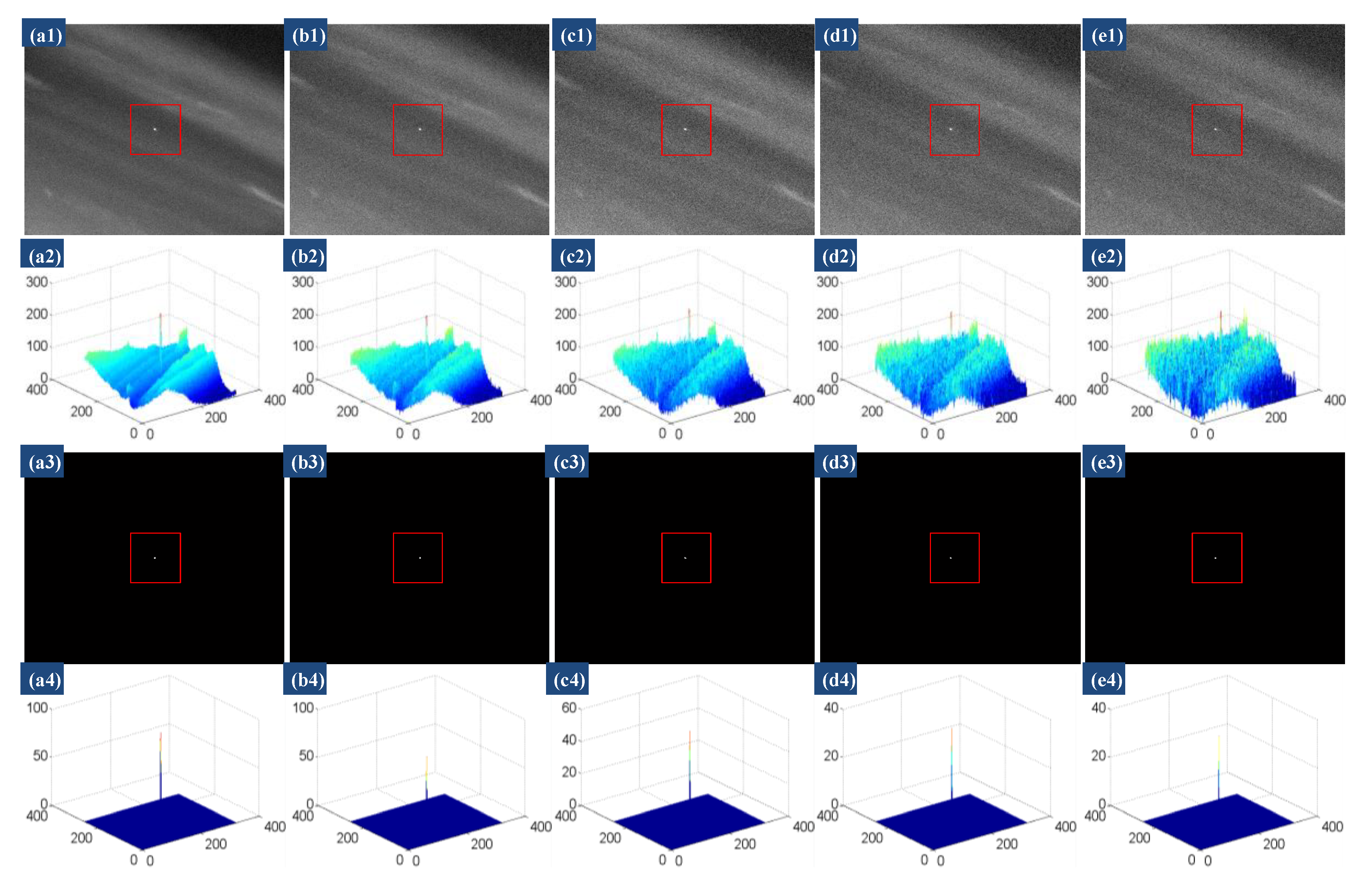
First, two infrared images (Scenes o and q) from Figure 7 were selected for our experiment and different Gaussian noises with mean 0 were added. We varied the standard deviation of the noise from 4 to 20 by an interval of 4 and obtained five image samples for each scene. Then, these image samples were processed to get the reconstructed target images by the proposed model. Experimental results of anti-noise are presented in Figure 14 and Figure 15 for the selected two scenes, respectively. In Figure 14 and Figure 15, the five images of the first row show the image samples added white Gaussian noise with standard deviation of 4, 8, 12, 16, and 20, respectively; the five images of the second row are the corresponding 3D mesh views of the image samples; the reconstructed target images by the proposed model; and their 3D mesh views are shown in third and fourth rows, respectively. From the experimental results, we can see that the proposed model significantly enhances the targets, and well suppresses the clutters and noise of the image samples simultaneously, if the standard deviation of noise is less than or equal to 16. As the standard deviation of noise increases to 20, it can be observed that our model still can detect the two targets, as shown in Figure 14e3 and Figure 15e3. An interference point (marked by the yellow square box) appears in Figure 14e3, but the little flaw is acceptable, because, in the 3D mesh view (Figure 14e4), we can observe that the grayscale of the true target is far much higher than that of the interference point. In other words, the above-mentioned experiment shows the robustness of our method with respect to the noise.

4.5. Quantitative Evaluation

In this subsection, the small target detection advantages of our method are further evaluated by quantitative indices including BSF, GSCR, ROC curve, computational time, etc. The six actual sequences of Table 1 were used as test set. Meanwhile, the six baseline methods were also tested and compared with our method.

In

Table 3. GSCR and BSF comparison of the seven methods for the representative frames of Sequence 1–6.

Method	32nd Frame of Sequence 1 GSCR BSF		18th Frame of Sequence 2 GSCR BSF		58th Frame of Sequence 3 GSCR BSF		103rd Frame of Sequence 4 GSCR BSF		29th Frame of Sequence 5 GSCR BSF		203rd Frame of Sequence 6 GSCR BSF
Top-hat	10.89	12.31	139.62	6.98	23.72	18.38	179.28	140.14	27.39	29.18	9.05	15.16
LCM	13.82	0.42	3.09	0.61	24.89	0.74	15.98	0.82	4.84	0.73	5.38	0.80
MPCM	31.41	1.67	1693.7	47.35	20.12	0.46	2996.3	328.60	88.12	17.03	131.79	36.92
IPI	3957.3	90734.1	1729.7	10865.3	1034.1	33076.2	INF	INF	—	—	2087.2	86371.2
RIPT	INF	INF	—	—	INF	INF	INF	INF	INF	INF	INF	INF
PSTNN	INF	INF	INF	INF	INF	INF	INF	INF	INF	INF	3482.6	55673.7
Ours	INF	INF	INF	INF	INF	INF	INF	INF	INF	INF	INF	INF

Notes: The representative frames of Sequence 1–6 have been shown in Figure 7o–t. The 32nd frame of Sequence 1 is Figure 7o; the 18th frame of Sequence 2 is Figure 7p; the 58th frame of Sequence 3 is Figure 7q; the 103rd frame of Sequence 4 is Figure 7r; the 29th frame of Sequence 5 is Figure 7s; and the 203rd frame of Sequence 5 is Figure 7t.

, BSF and GSCR values of the tested seven methods for the representative images of Sequences 1–6 are shown, where INF, namely infinity, indicates that the backgrounds of target neighborhood are completely swept away and shrink to zeros. It should be noted that we do not show GSCR and BSF values of IPI for the 29th frame of Sequence 5 and of RIPT for the 18th frame of Sequence 2, because the gray values of target pixels shrink to zeros in the processed images. In this case, the target cannot be detected, thus it is meaningless to calculate GSCR and BSF. Table 3 shows that our method has achieved the highest GSCR and BSF values on each sequence, showing the excellent ability in terms of target enhancement and background suppression. In general, we observe that the three methods (RIPT, PSTNN, and ours) combining local and nonlocal priors have achieved higher values than the three methods (top-hat, LCM, and MPCM) based on local prior only. IPI method based on non-local prior gets an intermediate value in most sequences. These indicate that combining local and non-local priors can dig out more useful image information to improve detection performance. In addition, RIPT and PSTNN have achieved the best results as the proposed method in most cases, but it can be observed that RIPT would shrink the target pixels to 0 for the 18th frame of Sequence 2 (actually, there are similar results in some other frames of this sequence), resulting in the target not being detected, and that PSTNN compared with the proposed method is slightly worse for Sequence 6, which contains extremely complex ground background. This illustrates the superiority of our method.

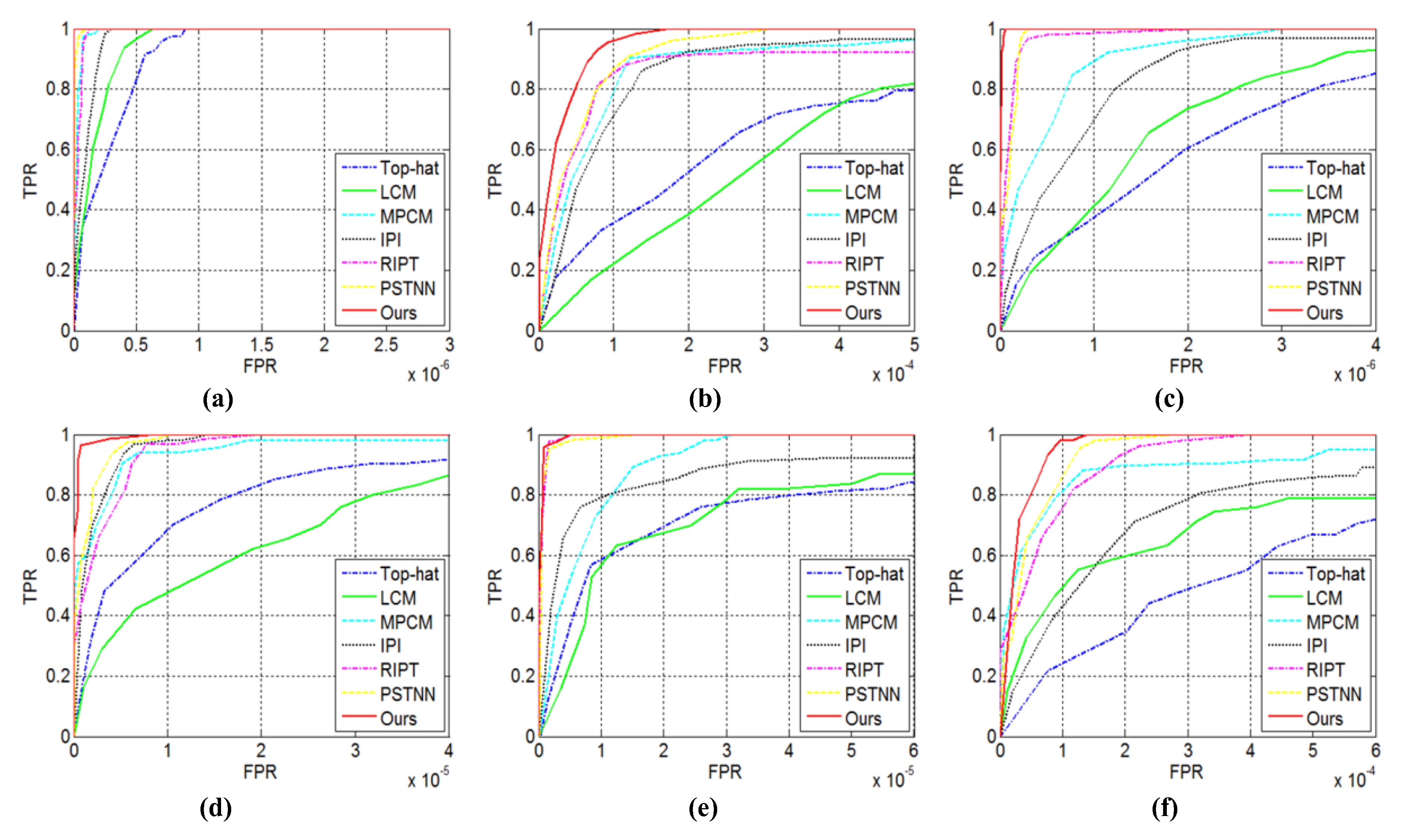
BSF and GSCR only reflect the background suppression and target enhancement abilities of detection method in a local region, not global image [23]. Therefore, to further verify the comprehensive detection performance of our algorithm, we obtained the ROC curves of those for the six sequences through experiments and compared them with the six other methods. In Figure 16, all the ROC curves are illustrated, and the corresponding AUC values are shown in

Table 4. AUC values of the seven methods on six sequences ($\times$ 10⁻⁶).

Method	Sequence 1	Sequence 2	Sequence 3	Sequence 4	Sequence 5	Sequence 6
Top-hat	999999.7425	794181.6994	852337.9990	916660.2614	840634.2914	719838.1942
LCM	999999.8425	814156.2798	931285.3525	864024.5811	866948.3188	787920.5486
MPCM	999999.9723	964616.2269	999999.5500	980992.2208	999993.0149	948777.5151
IPI	999999.9095	963380.2816	968361.9116	999998.1042	922509.7606	890273.9153
RIPT	999999.9678	922475.7108	999999.8932	999997.4886	999999.4593	999936.6724
PSTNN	999999.9931	999949.1340	999999.9091	999998.7491	999999.2596	999955.1185
Ours	1000000.0	999973.0608	999999.9917	999999.7070	999999.6314	999971.1846

Notes: Bold and underline represent the highest value and the second highest value in each sequence, respectively.

. The ROC curve that is the closer to the upper left corner and has the larger AUC value represents the better detection performance. In Figure 16 and Table 4, it can be observed that the detection performance of Top-hat is the worst in most sequences (except for Sequence 4), due to that the simple structural elements cannot handle the complex background and varying target. LCM based on local contrast performs slightly better than top-hat. MPCM is a derived version of LCM, thus it has great performance improvement; however, its performance is still worse than PSTNN and the proposed method for all sequences. IPI works well, but its performance is fluctuating. RIPT can achieve good results in most cases, but its performance is slightly worse on Sequence 2, because it would over-shrink the target in some cases. Overall, PSTNN and the proposed method have achieved the two best results, but it can be clearly seen that our method almost invariably has maximal TPR value in respect of the identical FPR and has the largest AUC value. All these demonstrate the proposed method has the most robust detection performance.

In addition to good detection ability, computational time is an important factor to be considered for infrared small target detection. Thus, the average single frame computational time of each method on six real sequences was also tested, and the test results are shown in

Table 5. Comparison of the single frame computation time (unit: s) for the seven methods.

Method	Sequence 1	Sequence 2	Sequence 3	Sequence 4	Sequence 5	Sequence 6
Top-hat	0.0806	0.0840	0.0814	0.0841	0.0864	0.0817
LCM	0.2536	0.2521	0.2562	0.2550	0.2528	0.2539
MPCM	0.2920	0.2989	0.2976	0.2928	0.2997	0.2901
IPI	24.8471	26.3660	23.5119	22.6283	8.1903	17.2996
RIPT	2.9696	1.2252	4.4051	1.8489	1.8196	1.7307
PSTNN	0.1474	0.6687	0.3471	0.6511	0.6148	0.5380
Ours	0.2838	0.3614	0.3111	0.3997	0.3680	0.3257

. We can observe that our method is slightly slower than the filtering methods (Top-hat, LCM and MPCM) utilizing local prior merely, but much faster than the similar optimizing methods (IPI, RIPT, and PSTTN) based on sparse and low-rank decomposition on all sequences, except for PSTNN in Sequence 1. Considering that the detection ability of our method greatly outperforms those filtering methods, it is obviously acceptable. IPI model is the slowest, resulting from high time-consuming accelerated proximal gradient (APG) approach [71], while the other optimizing methods are based on faster ADMM. Moreover, the processing time of RIPT and PSTNN fluctuate greatly for different scenes, while our method is relatively stable. This is also very important for practical application systems.

5. Conclusions

In this paper, a patch-tensor model with non-convex tensor rank surrogate, local contrast energy, and structured sparse regularization, namely, NTRS, is proposed for small infrared target detection. In the proposed model, the Laplace function based non-convex approximation for ${\ell }_1$-norm of the tensor multi-rank is utilized to measure the low-rank characteristic of the background patch-tensor, so as to separate target and background more robustly. Considering that the local prior map can be equivalent to the saliency map, the local contrast energy feature as prior information is introduced to weight sparse target patch-tensor. To further wipe out those stubborn rare structures, an additional tube-wise sparse tensor regularization term is introduced into our detection model. Finally, target detection task is formulated as a separation problem of low-rank, sparse, and structured sparse tensors, which is solved via an optimization algorithm based on ADMM and the fast t-SVD. In addition, the key parameters of the model can be selected appropriately through experiments. Extensive experimental results of various scenes and real sequences verify that our approach is robust and achieves excellent detection ability, and outperforms the other advanced approaches. Moreover, our approach is competitive in processing time with respect to other widely used methods. In the future, we can further explore detection techniques based on local contrast and merge them into IPT detection framework, such as multi-scale technique.

References

1. Huang, S.Q.; Liu, Y.H.; He, Y.M.; Zhang, T.F.; Peng, Z.M. Structure-Adaptive Clutter Suppression for Infrared Small Target Detection: Chain-Growth Filtering. Remote Sens. 2020, 12, 47. [Google Scholar] [CrossRef] [Green Version]
2. Wang, X.Y.; Peng, Z.M.; Kong, D.H.; Zhang, P.; He, Y.M. Infrared dim target detection based on total variation regularization and principal component pursuit. Image Vis. Comput. 2017, 63, 1–9. [Google Scholar] [CrossRef]
3. Wang, X.Y.; Peng, Z.M.; Kong, D.H.; He, Y.M. Infrared Dim and Small Target Detection Based on Stable Multisubspace Learning in Heterogeneous Scene. IEEE Trans. Geosci. Remote. 2017, 55, 5481–5493. [Google Scholar] [CrossRef]
4. Huang, S.Q.; Peng, Z.m.; Wang, Z.R.; Wang, X.Y.; Li, M.H. Infrared Small Target Detection by Density Peaks Searching and Maximum-Gray Region Growing. IEEE Geosci. Remote Sens. Lett. 2019, 16, 1919–1923. [Google Scholar] [CrossRef]
5. Zhang, T.F.; Wu, H.; Liu, Y.; Peng, L.B.; Yang, C.P.; Peng, Z.M. Infrared Small Target Detection Based on Non-Convex Optimization with Lp-Norm Constraint. Remote Sens. 2019, 11, 559. [Google Scholar] [CrossRef] [Green Version]
6. Peng, Z.M.; Zhang, Q.H.; Wang, J.R.; Zhang, Q.P. Dim target detection based on nonlinear multifeature fusion by Karhunen-Loeve transform. Opt. Eng. 2004, 43, 2954–2958. [Google Scholar] [CrossRef]
7. Li, X.; Wang, J.; Li, M.H.; Peng, Z.M.; Liu, X.R. Investigating Detectability of Infrared Radiation Based on Image Evaluation for Engine Flame. Entropy 2019, 21, 946. [Google Scholar] [CrossRef] [Green Version]
8. Zhang, L.D.; Peng, Z.M. Infrared Small Target Detection Based on Partial Sum of the Tensor Nuclear Norm. Remote Sens. 2019, 11, 382. [Google Scholar] [CrossRef] [Green Version]
9. Xia, C.Q.; Li, X.R.; Zhao, L.Y. Infrared small target detection via modified random walks. Remote Sens. 2018, 10, 2004. [Google Scholar] [CrossRef] [Green Version]
10. Wei, Y.T.; You, X.G.; Li, H. Multiscale patch-based contrast measure for small infrared target detection. Pattern Recogn. 2016, 58, 216–226. [Google Scholar] [CrossRef]
11. Qi, H.; Mo, B.; Liu, F.; He, Y.; Liu, S.D. Small infrared target detection utilizing local region similarity difference map. Infrared Phys. Technol. 2015, 71, 131–139. [Google Scholar] [CrossRef]
12. Reed, I.S.; Gagliardi, R.M.; Stotts, L.B. Optical moving target detection with 3-D matched filter. IEEE Trans. Aerosp. Electorn. Syst. 2002, 24, 327–336. [Google Scholar] [CrossRef]
13. Wang, G.; Inigo, R.M.; Mcvey, E.S. A pipeline algorithm for detection and tracking of pixel-sized target trajectories. In Proceedings of the Signal and Data Processing of Small Targets, Orlando, FL, USA, 1 October 1990; pp. 167–178. [Google Scholar]
14. Modestino, J.W. Spatiotemporal multiscan adaptive matched filtering. In Signal and Data Processing of Small Targets; International Society for Optics and Photonics: Bellingham, WA, USA, 1995. [Google Scholar]
15. Tonissen, S.M.; Evans, R.J. Performance of dynamic programming techniques for Track-Before-Detect. IEEE Trans. Aerosp. Electorn. Syst. 1996, 32, 1440–1451. [Google Scholar] [CrossRef]
16. Gao, C.Q.; Zhang, T.Q.; Li, Q. Small infrared target detection using sparse ring representation. IEEE Aerosp. Electron. Syst. Mag. 2012, 27, 21–30. [Google Scholar]
17. Gao, C.Q.; Wang, L.; Xiao, Y.X.; Zhao, Q.; Meng, D.Y. Infrared small-dim target detection based on Markov random field guided noise modeling. Pattern Recogn. 2018, 76, 463–475. [Google Scholar] [CrossRef]
18. Zhang, H.; Zhang, L.; Yuan, D.; Chen, H. Infrared small target detection based on local intensity and gradient properties. Infrared Phys. Technol. 2018, 89, 88–96. [Google Scholar] [CrossRef]
19. Wang, X.Y.; Peng, Z.M.; Zhang, P.; He, Y.M. Infrared Small Target Detection via Nonnegativity-Constrained Variational Mode Decomposition. IEEE Geosci. Remote Sens. Lett. 2017, 14, 1700–1704. [Google Scholar] [CrossRef]
20. Liu, D.P.; Cao, L.; Li, Z.Z.; Liu, T.M.; Che, P. Infrared Small Target Detection Based on Flux Density and Direction Diversity in Gradient Vector Field. IEEE J-Stars. 2018, 11, 2528–2554. [Google Scholar] [CrossRef]
21. Peng, L.B.; Zhang, T.F.; Liu, Y.H.; Li, M.H.; Peng, Z.M. Infrared Dim Target Detection Using Shearlet’s Kurtosis Maximization under Non-Uniform Background. Symmetry 2019, 11, 723. [Google Scholar] [CrossRef] [Green Version]
22. Peng, L.B.; Zhang, T.F.; Huang, S.Q.; Pu, T.; Liu, Y.H.; Lv, Y.X.; Zheng, Y.C.; Peng, Z.M. Infrared Small Target Detection Based on Multi-directional Multi-scale High Boost Response. Opt. Rev. 2019, 26, 568–582. [Google Scholar] [CrossRef]
23. Dai, Y.M.; Wu, Y.Q. Reweighted Infrared Patch-Tensor Model with Both Nonlocal and Local Priors for Single-Frame Small Target Detection. IEEE J-Stars. 2017, 10, 3752–3767. [Google Scholar] [CrossRef] [Green Version]
24. Li, W.; Zhao, M.; Deng, X.; Li, L.; Li, L.; Zhang, W. Infrared Small Target Detection Using Local and Nonlocal Spatial Information. IEEE J. Sel. Top. Appl. Earth Observ. Remote Sens. 2019, 12, 3677–3689. [Google Scholar] [CrossRef]
25. Deshpande, S.D.; Er, M.H.; Venkateswarlu, R.; Chan, P. Max-mean and max-median filters for detection of small targets. In Proceedings of the Signal and Data Processing of Small Targets, Denver, CO, USA, 18–23 July 1999; pp. 74–84. [Google Scholar]
26. Hadhoud, M.M.; Thomas, D.W. The two-dimensional adaptive LMS (TDLMS) algorithm. IEEE Trans. Circuits Syst. 1988, 35, 485–494. [Google Scholar] [CrossRef]
27. Tom, V.T.; Peli, T.; Leung, M.; Bondaryk, J.E. Morphology-based algorithm for point target detection in infrared backgrounds. In Proceedings of the Signal and Data Processing of Small Targets, Orlando, FL, USA, 22 October 1993; pp. 2–12. [Google Scholar]
28. Bae, T.W.; Zhang, F.; Kweon, I.S. Edge directional 2D LMS filter for infrared small target detection. Infrared Phys. Technol. 2012, 55, 137–145. [Google Scholar] [CrossRef]
29. Cao, Y.; Liu, R.M.; Yang, J. Small target detection using two-dimensional least mean square (TDLMS) filter based on neighborhood analysis. Int. J. Infrared Milli. 2008, 29, 188–200. [Google Scholar] [CrossRef]
30. Ye, Z.; Ruan, Y.; Wang, J.; Zou, Y. Detection algorithm of weak infrared point targets under complicated background of sea and sky. Infrared Millimeter Terahertz Waves. 2000, 19, 121–124. [Google Scholar]
31. Gu, Y.F.; Wang, C.; Liu, B.X.; Zhang, Y. A kernel-based nonparametric regression method for clutter removal in infrared small-target detection applications. IEEE Trans. Geosci. Remote Sens. Lett. 2010, 7, 469–473. [Google Scholar] [CrossRef]
32. Wang, H.; Yang, F.; Zhang, C.; Ren, M. Infrared Small Target Detection Based on Patch Image Model with Local and Global Analysis. Int. J. Image Graph. 2018, 18, 1850002. [Google Scholar] [CrossRef]
33. Kim, S.; Yang, Y.; Lee, J.; Park, Y. Small target detection utilizing robust methods of the human visual system for IRST. Infrared Milli. Terahertz Waves 2009, 30, 994–1011. [Google Scholar] [CrossRef]
34. Chen, C.P.; Li, H.; Wei, Y.T.; Xia, T.; Tang, Y.Y. A local contrast method for small infrared target detection. IEEE Trans. Geosci. Remote Sens. 2013, 52, 574–581. [Google Scholar] [CrossRef]
35. Shi, Y.F.; Wei, Y.T.; Yao, H.; Pan, D.H.; Xiao, G.R. High-Boost-Based Multiscale Local Contrast Measure for Infrared Small Target Detection. IEEE Geosci. Remote Sens. Lett. 2018, 15, 33–37. [Google Scholar] [CrossRef]
36. Du, P.; Hamdulla, A. Infrared Small Target Detection Using Homogeneity-Weighted Local Contrast Measure. IEEE Geosci. Remote Sens. Lett. 2019. [Google Scholar] [CrossRef]
37. Bai, X.Z.; Bi, Y.G. Derivative entropy-based contrast measure for infrared small-target detection. IEEE Trans. Geosci. Remote Sens. 2018, 56, 2452–2466. [Google Scholar] [CrossRef]
38. Gao, C.Q.; Meng, D.Y.; Yang, Y.; Wang, Y.T.; Zhou, X.F.; Hauptmann, A.G. Infrared Patch-Image Model for Small Target Detection in a Single Image. IEEE Trans. Image Process. 2013, 22, 4996–5009. [Google Scholar] [CrossRef]
39. Dai, Y.M.; Wu, Y.Q.; Song, Y. Infrared small target and background separation via column-wise weighted robust principal component analysis. Infrared Phys. Technol. 2016, 77, 421–430. [Google Scholar] [CrossRef]
40. Dai, Y.M.; Wu, Y.Q.; Song, Y.; Guo, J. Non-negative infrared patch-image model: Robust target-background separation via partial sum minimization of singular values. Infrared Phys. Technol. 2017, 81, 182–194. [Google Scholar] [CrossRef]
41. Guo, J.; Wu, Y.Q.; Dai, Y.M. Small target detection based on reweighted infrared patch-image model. IET Image Process. 2018, 12, 70–79. [Google Scholar] [CrossRef]
42. Zhang, L.D.; Peng, L.B.; Zhang, T.F.; Cao, S.Y.; Peng, Z.M. Infrared Small Target Detection via Non-Convex Rank Approximation Minimization Joint l2,1 Norm. Remote Sens. 2018, 10, 1821. [Google Scholar] [CrossRef] [Green Version]
43. Sun, Y.; Yang, J.G.; Long, Y.L.; Shang, Z.R.; An, W. Infrared Patch-Tensor Model with Weighted Tensor Nuclear Norm for Small Target Detection in a Single Frame. IEEE Access 2018, 6, 76140–76152. [Google Scholar] [CrossRef]
44. Goldfarb, D.; Qin, Z.W. Robust Low-Rank Tensor Recovery: Models and Algorithms. Siam J. Matrix Anal. Appl. 2014, 35, 225–253. [Google Scholar] [CrossRef] [Green Version]
45. Xu, W.H.; Zhao, X.L.; Ji, T.Y.; Miao, J.Q.; Ma, T.H. Laplace function based nonconvex surrogate for low-rank tensor completion. Signal Process. Image Commun. 2019, 73, 62–69. [Google Scholar] [CrossRef]
46. Romera-Paredes, B.; Pontil, M. A new convex relaxation for tensor completion. In Proceedings of the Advances in Neural Information Processing Systems, Harrahs and Harveys, Lake Tahoe, NV, USA, 5–10 December 2013; pp. 2967–2975. [Google Scholar]
47. Lu, C.; Feng, J.; Chen, Y.; Liu, W.; Lin, Z.; Yan, S. Tensor robust principal component analysis: Exact recovery of corrupted low-rank tensors via convex optimization. In Proceedings of the IEEE Conference on Computer Vision and Pattern Recognition, Las Vegas, NV, USA, 27–30 June 2016; pp. 5249–5257. [Google Scholar]
48. Semerci, O.; Hao, N.; Kilmer, M.E.; Miller, E.L. Tensor-based formulation and nuclear norm regularization for multienergy computed tomography. IEEE Trans. Image Process. 2014, 23, 1678–1693. [Google Scholar] [CrossRef] [PubMed] [Green Version]
49. Zhang, X.Y.; Ding, Q.H.; Luo, H.B.; Hui, B.; Chang, Z.; Zhang, J.C. Infrared small target detection based on an image-patch tensor model. Infrared Phys. Technol. 2019, 99, 55–63. [Google Scholar] [CrossRef]
50. Zhang, Z.M.; Ely, G.; Aeron, S.; Hao, N.; Kilmer, M. Novel methods for multilinear data completion and de-noising based on tensor-SVD. In Proceedings of the IEEE Conference on Computer Vision and Pattern Recognition, Columbus, OH, USA, 23–28 June 2014; pp. 3842–3849. [Google Scholar] [CrossRef] [Green Version]
51. Kilmer, M.E.; Martin, C.D. Factorization strategies for third-order tensors. Linear Algebra Appl. 2011, 435, 641–658. [Google Scholar] [CrossRef] [Green Version]
52. Martin, C.D.; Shafer, R.; LaRue, B. An order-p tensor factorization with applications in imaging. SIAM J. Sci. Comput. 2013, 35, A474–A490. [Google Scholar] [CrossRef]
53. Kilmer, M.E.; Braman, K.; Hao, N.; Hoover, R.C. Third-order tensors as operators on matrices: A theoretical and computational framework with applications in imaging. SIAM J. Matrix Anal. Appl. 2013, 34, 148–172. [Google Scholar] [CrossRef] [Green Version]
54. Lu, C.; Feng, J.; Chen, Y.; Liu, W.; Lin, Z.; Yan, S. Tensor Robust Principal Component Analysis with A New Tensor Nuclear Norm. IEEE Trans. Pattern Anal. Mach. Intell. 2019. [Google Scholar] [CrossRef] [Green Version]
55. Zhang, Z.M.; Aeron, S.C. Exact tensor completion using t-SVD. IEEE Trans. Signal Process. 2017, 65, 1511–1526. [Google Scholar] [CrossRef]
56. Carroll, J.D.; Chang, J.-J. Analysis of individual differences in multidimensional scaling via an N-way generalization of “Eckart-Young” decomposition. Psychometrika 1970, 35, 283–319. [Google Scholar] [CrossRef]
57. Tucker, L.R. Some mathematical notes on three-mode factor analysis. Psychometrika 1966, 31, 279–311. [Google Scholar] [CrossRef]
58. Kolda, T.G.; Bader, B.W. Tensor decompositions and applications. SIAM Rev. 2009, 51, 455–500. [Google Scholar] [CrossRef]
59. Oh, T.H.; Tai, Y.W.; Bazin, J.C.; Kim, H.; Kweon, I.S. Partial sum minimization of singular values in robust PCA: Algorithm and applications. IEEE Trans. Pattern Anal. Mach. Intell. 2016, 38, 744–758. [Google Scholar] [CrossRef] [PubMed] [Green Version]
60. Jiang, T.-X.; Huang, T.-Z.; Zhao, X.-L.; Deng, L.-J. A novel nonconvex approach to recover the low-tubal-rank tensor data: When t-SVD meets PSSV. arXiv 2018, arXiv:1712.05870v2 [cs.NA]. [Google Scholar]
61. Chen, Y.; Guo, Y.; Wang, Y.; Wang, D.; Peng, C.; He, G. Denoising of hyperspectral images using nonconvex low rank matrix approximation. IEEE Trans. Geosci. Remote Sens. 2017, 55, 5366–5380. [Google Scholar] [CrossRef]
62. Benedek, C.; Descombes, X.; Zerubia, J. Building Development Monitoring in Multitemporal Remotely Sensed Image Pairs with Stochastic Birth-Death Dynamics. IEEE Trans. Pattern Anal. 2012, 34, 33–50. [Google Scholar] [CrossRef] [Green Version]
63. Candes, E.J.; Wakin, M.B.; Boyd, S.P. Enhancing Sparsity by Reweighted l1 Minimization. J. Fourier Anal. Appl. 2008, 14, 877–905. [Google Scholar] [CrossRef]
64. Gu, S.H.; Zhang, L.; Zuo, W.M.; Feng, X.C. Weighted Nuclear Norm Minimization with Application to Image Denoising. In Proceedings of the IEEE Conference on Computer Vision and Pattern Recognition, Columbus, OH, USA, 23–28 June 2014; pp. 2862–2869. [Google Scholar] [CrossRef] [Green Version]
65. Peng, Y.; Suo, J.; Dai, Q.; Xu, W. Reweighted low-rank matrix recovery and its application in image restoration. IEEE Trans. Cybern. 2014, 44, 2418–2430. [Google Scholar] [CrossRef]
66. Lu, C.Y.; Tang, J.H.; Yan, S.C.; Lin, Z.C. Nonconvex Nonsmooth Low Rank Minimization via Iteratively Reweighted Nuclear Norm. IEEE Trans. Image Process. 2016, 25, 829–839. [Google Scholar] [CrossRef] [Green Version]
67. Boyd, S.; Parikh, N.; Chu, E.; Peleato, B.; Eckstein, J. Distributed optimization and statistical learning via the alternating direction method of multipliers. Found. Trends Mach. Learn. 2011, 3, 1–122. [Google Scholar] [CrossRef]
68. Lin, Z.; Chen, M.; Ma, Y. The augmented lagrange multiplier method for exact recovery of corrupted low-Rank matrices. arXiv 2010, arXiv:1009.5055v1. [Google Scholar]
69. Bouwmans, T.; Javed, S.; Zhang, H.Y.; Lin, Z.C.; Otazo, R. On the Applications of Robust PCA in Image and Video Processing. Proc. IEEE. 2018, 106, 1427–1457. [Google Scholar] [CrossRef] [Green Version]
70. Guan, X.W.; Peng, Z.M.; Huang, S.Q.; Chen, Y.P. Gaussian Scale-Space Enhanced Local Contrast Measure for Small Infrared Target Detection. IEEE Geosci. Remote Sens. Lett. 2020, 17, 327–331. [Google Scholar] [CrossRef]
71. Lin, Z.; Ganesh, A.; Wright, J.; Wu, L.; Chen, M.; Ma, Y. Fast convex optimization algorithms for exact recovery of a corrupted low-rank matrix. In Proceedings of the CAMSAP 2009, Aruba, Dutch Antilles, 13–16 December 2009; pp. 1–18. [Google Scholar]
Figure 1. T-SVD illustration of a third-order tensor X m 1 × m 2 × m 3 . U ,   S , V are third-order tensors of size m 1 × m 2 × m 3 , m 1 × m 2 × m 3 , and m 2 × m 2 × m 3 , respectively.   S is also a f-diagonal tensor.
Remotesensing 12 01520 g001
Figure 2. Tensor construction. The left is to obtain local patch-images and these patches are stacked as a third-order tensor on the right. The red arrow indicates sliding operation. m 3 is the number of patches.
Remotesensing 12 01520 g002
Figure 3. Comparison of the contribution of the 1 -norm, the Laplace function, and 0 -norm to the rank with respect to a varying singular value.
Remotesensing 12 01520 g003
Figure 4. Constructing of the local contrast element: (a) a sub-block in the whole image; and (b) the diffusion structure of the sub-block. B ( x , y ) k is a set of all neighborhood pixels with a distance of k from the center pixel ( x , y ) , and is indicated with dotted lines of different colors.
Remotesensing 12 01520 g004
Figure 5. (a) Raw infrared image; (b) local prior weight map of PSTNN, where there are some strong edge residuals left in the red circle; and (c) the proposed local prior weight map.
Remotesensing 12 01520 g005
Figure 6. The flowchart of the proposed infrared small target detection method. First, local prior weight map is generated by using local contrast energy feature. Second, original patch-tensor and local prior weight patch-tensor are constructed. Third, the low-rank background tensor , the structured sparse edge tensor S , and the sparse target tensor T can be separated by the proposed model. Then, the target image is reconstructed and small targets can be extracted by an adaptive threshold segmentation algorithm.
Remotesensing 12 01520 g006
Figure 7. The 20 original infrared images of different scenes used in the experiment. A red square indicates that there is a real target in the area.
Remotesensing 12 01520 g007
Figure 8. Corresponding 3D mesh views of the 20 different scenes in Figure 7. The images in (at) correspond to Figure 7a–t, respectively. The x-axis and y-axis represent the column coordinate and row coordinate of the pixels of the original image, respectively, while the z-axis represents the gray value of the pixels.
Remotesensing 12 01520 g008
Figure 9. An infrared small target and its local adjacent area. Yellow rectangle denotes the small target area and red rectangle denotes its local adjacent area. On the right is an enlarged view of the red rectangle.
Remotesensing 12 01520 g009
Figure 10. Detection performances of the proposed model under different parameters for the six tested sequences: (a1a6) ROC curves under different patch sizes on Sequence 1–6; (b1b6) ROC curves under different sliding steps on Sequence 1–6; (c1c6) ROC curves under different penalty factors on Sequence 1–6; and (d1d6) ROC curves under different compromising parameters on Sequences 1–6.
Remotesensing 12 01520 g010aRemotesensing 12 01520 g010b
Figure 11. Twenty reconstructed target images by the proposed model. Red Squares indicate the detected true targets. (at) The processed results corresponding to the original images in Figure 7a–t, respectively. All the true targets are accurately detected without any false alarm.
Remotesensing 12 01520 g011
Figure 12. 3D mesh views of the reconstructed target images in Figure 11. The images in (at) correspond to Figure 11a–t, respectively. In each subfigure, the x-axis and y-axis represent the column coordinate and row coordinate of the pixels of the original image, respectively, while the z-axis represents the gray value of the pixels.
Remotesensing 12 01520 g012
Figure 13. Twenty processed target images by PSTNN model. The images in (at) correspond to the original images in Figure 7a–t, respectively. Red Squares denote the detected targets. Yellow rectangles and squares denote the residual clutters that may cause false alarms and their enlarged views are also shown to facilitate observation.
Remotesensing 12 01520 g013
Figure 14. Experimental results of anti-noise for the scene in Figure 7o by the proposed model: (a1e1) the image samples added white Gaussian noise with standard deviations of 4, 8, 12, 16, and 20; (a2e2) 3D mesh views of the image samples; (a3e3) the reconstructed target images; and (a4e4) 3D mesh views of the reconstructed target images. Red Squares denote the true targets detected. Yellow square denotes the residual clutter in the reconstructed target image. In (a2e2,a4e4), the horizontal plane represents the coordinate location of the image pixels, and the height dimension represents the gray value of the pixels.
Remotesensing 12 01520 g014
Figure 15. Experimental results of anti-noise for the scene in Figure 7q by the proposed model: (a1e1) the image samples added white Gaussian noise with standard deviation of 4, 8, 12, 16, 20; (a2e2) 3D mesh views of the image samples; (a3e3) the reconstructed target images; and (a4e4) 3D mesh views of the reconstructed target images. Red Squares denote the true targets detected. In (a2e2,a4e4), the horizontal plane represents the coordinate location of the image pixels, and the height dimension represents the gray value of the pixels.
Remotesensing 12 01520 g015
Figure 16. ROC curves of detection results under different methods on the six tested sequences: (a) ROC curves on Sequence 1; (b) ROC curves on Sequence 2; (c) ROC curves on Sequence 3; (d) ROC curves on Sequence 4; (e) ROC curves on Sequence 5; and (f) ROC curves on Sequence 6. Blue dash-dot line, green solid line, cyan dashed line, black dotted line, magenta dash-dot line, yellow dashed line, and red solid line are used for Top-hat, LCM, MPCM, IPI, RIPT, PSTNN, and our method, respectively.
Remotesensing 12 01520 g016