Creation of One Excavator as an Obstacle in C-Space for Collision Avoidance during Remote Control of the Two Excavators Using Pose Sensors

Abstract

Many solutions about the teleoperation of unmanned robotic excavators have been studied continuously. However, if excavators that are remotely controlled were employed, the probability of an accident would be higher. For this reason, there have been many ways proposed to attempt to reduce accidents in these dangerous situations. In this paper, a novel methodology will be introduced with a focus on the multiple excavators themselves. The proposed method details how one excavator can be generated or expressed as an obstacle in the Configuration-Space (C-space) with respect to another excavator’s side for collision avoidance each other. This method is based on kinematics information which is measurable and given. Therefore, this method can be used or applied independently by using widely used pose sensors and wireless communication devices. The phase of mathematical derivation about obstacle sets is described in detail. The results are shown in accompanying figures and tables for demonstrating that the proposed method detected the proximity and found the collision-free zone accurately. The proposed system can be powerful when applied to a teleoperation system, where it would be particularly useful and helpful to the operator.

1. Introduction

The typical excavator uses a hydraulic actuator and variable attachments, so its applications are unlimited. For this reason, it can be widely used in many fields such as construction, mining, and agriculture, and in more dangerous places for rescue and recovery operations. Note that the excavator is often employed in areas where multi-excavator cooperation is required. Sometimes cooperation may be required, such as lifting an object or moving an object. However, these factors can create some dangerous situations such as an unpredictable collision with each excavator, which is one of the most common and fatal accidents. In order to prevent these types of accidents, operators, workers-on-foot, and managers should maintain visual awareness to avoid collisions and notify warning while driving and manipulating an excavator. Therefore, in recent years, the demand for system management for safety management is increasing. Furthermore, the safety factor has gradually become an essential point because a recent trend is developing unmanned robotic excavators.

There have been many ways to attempt to reduce collision accident in these dangerous situations. Unfortunately, under conditions when sensor systems were poor, some local problems had been found in existing solutions. The accuracy of these problems could be reduced if environments were bad, such as interference from installations of many devices or too much unpredictable particles. In contrast with the past, many great developments of prevention and warning systems exist today. Moreover, compared to the proposed method, there are some significant differences in these systems. Almost of them had primarily focused on the side of the workers-on-foot and single excavator.

The proposed method details how one typical excavator can be expressed as an obstacle numerically in the C-space with respect to another excavator’s side. It will focus on the side of not only workers, but also multiple excavators themselves. The obstacles are generated in the three defined types of C-space as images so that they could be used as a supplementary index for workers or multiple robotic excavators in avoiding a collision more precisely.

Most of all, this method is based on kinematics information, which is measurable and given. Therefore, in the case of role of an index, the proposed method can be used independently or in combination with existing warning and detection solutions by using widely used sensor devices. This is the reason why this paper developed the kinematics-based method to achieve the objective. Because compatibility and versatile application would be higher, many solutions and devices based on the kinematics have been developed and widely used.

Nowadays, it is common that GPS and inertial measurement unit (IMU) sensor devices are used for machine guidance and control. Therefore, GPS and IMU devices were used for gathering kinematics information and demonstration of the proposed method. The real-time solution depends on the specifications of the sensors and the communication system. The paper will also include parameters related to the time domain.

Furthermore, many solutions for the teleoperation of unmanned robotic excavators have been studied for some time. Trivially, it would be better if the proposed method is applied to a teleoperation system when multiple excavators are deployed.

The outline of this paper is as follows. In Section 2, the analysis of previous works will be described. Through Section 2, the validity of the principal contribution of this paper will be described in detail. The mathematical derivations of the proposed method will be explained in Section 3, and it will be verified through the simulations in Section 4. Section 5 will show the actual tests and results, and this paper will end with a discussion and conclusion in the last section.

2. Literature Review

Preventing collisions is a very important factor in the cooperation of construction machines as well as cooperative robot systems. In robotics, many methods about motion or path planning for collision free of the multiple robot manipulators have already been studied for some time. For example, these works in [1,2,3,4,5,6,7,8,9,10] explain path and motion planning methods for collision avoidance. There are two main points in these papers. The one is that obstacle generation in the C-space is a necessary condition for performing collision avoidance. The other one is that obstacles must be generated in C-space for motion or path planning.

Therefore, a method of efficiently generating obstacles has also been studied. Ge derived the equations for the boundaries of joint obstacles for planar robots [11]. Dooley also described the joint space obstacles for a 5R closed chain robot [12]. Branicky studied a method for the rapid computation of configuration space obstacles [13]. In on-line methodology, Newman developed a real-time configuration space transform [14]. Nowadays, an optimal configuration construction method has been developed by Pan [15].

Of course, many studies about proximity warning systems and prevention of collisions for path planning of cooperative heavy-duty machines have also been conducted. More papers on applications in the construction field will be reviewed in the next paragraph.

GPS has been used in mining to improve safety by avoiding collisions. Antonio and Ruff developed a safety system based on GPS [16,17,18,19]. Ruff also studied a radar-based proximity warning system for off-highway dump trucks [20]. Kamat presented research that investigated the implementation of the fast and interactive collision detection method [21]. Proximity sensing through the use of an RF module was developed by Marks [22,23]. This system is economical and has a wide range of applications. In case of the use of magnetic materials, Teizer has developed magnetic field proximity detection and alert technology for safe operation [24]. Golovina has developed a method about preventing struck-by between workers-on-foot and construction equipment by generating the heat maps [25]. Wang presented a novel approach to reduce false alarms by adopting the four-dimensional space [26]. A method without using sensor devices was devised. Sivakumar and Ali studied collision-free path planning of cooperative crane manipulators using kinematic information with a heuristic or genetic algorithm [27,28]. Sivakumar and Ali used configuration space for collision free. It is also remarkable that C-Space is one of the important elements for collision avoidance in construction sites. The use of C-Space in construction field can be found in the following papers [29,30].

Safety systems applied to excavators can be also found easily. RFID technology has been used to prevent collision accidents [31,32]. Teizer mainly used radio frequency (RF), light detection and ranging (LIDAR), and position data to implement an autonomous proactive real-time system [33]. A visualization awareness about risk situations project using augmented reality (AR) was proposed by Su [34]. Vahdatikhaki suggested a risk map generation considering the visibility and proximity-based hazards using pose information and Near-Real-Time Simulation [35]. Shen designed a hazard zone around construction equipment in which site personnel should not be during operations [36]. Gonon applied the potential field method in order to avoid collisions when controlling the excavator [37].

However, the reviewed method left somethings to be desired. Most of all, there is no methodology for avoiding collisions that focus on multiple excavators during cooperation. The scope is primarily occasions that would occur between excavators and workers or other vehicles, not each excavator. In addition, many solutions were based primarily on vision systems. Papers presented by Mastalli and Vahdatikhaki are examples [38,39]. However, some computation processes should be included for generating exact and necessary data into the joint space in order to implement planning.

The proposed method is dedicated to things that can be used for collision avoidance during the cooperation of multiple excavators. In other words, as described earlier, it can be used for the index of guidance systems in collision avoidance. It is also great potential to be a supplementary tool if it used with existing solutions.

3. Methdology

Each excavator must recognize the others as obstacles for collision avoidance during cooperation to ensure safety in a broad workspace. As this method is dedicated to just multiple excavators, this section will details how one excavator can be expressed as an obstacle numerically with respect to another excavator’s side. A varied C-space including joint space was selected for obstacle generation with consideration for robotic application. A numerical computation based on a geometric approach with kinematics will be used throughout the overall phase of derivation.

The proposed method will be explained based on the conditions and assumptions as follows.

• The target to be expressed as an obstacle is just a typical excavator. The rest such as unknown debris are excluded because it becomes a meaningless object in the computation.
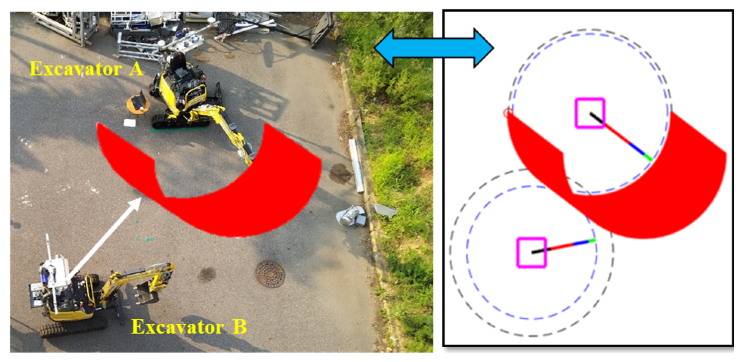
• Two excavators recognize each other as obstacles. However, from this point, the target excavator that will be the obstacle will be called “A” so that “B” will recognize Excavator A as an obstacle.
• Only kinematic information will be used. Therefore, the posture of the two excavators must be known, given, and measurable.
• The methodology is divided into two parts: when driving, and when manipulating the boom, stick, bucket, and swing.
• All links and the body are treated as segments for the computations.

Section 3.1 is about driving, and Section 3.2 is about link manipulation for guidance without collisions.

3.1. Obstacle Generation for Driving Guidance

Two excavators are on the ground arbitrarily in Figure 1. When one excavator is working far away from the other one, trivially, they do not have to consider the posture of other. If not, the operator should control the excavator for collision avoidance by considering the posture of the other excavator.

When driving, one excavator ”B” must know the exact position area of the other excavator “A”, which could be involved in a collision situation. Therefore, the ${\mathbb{R}}^2$ is selected for expressing the generated obstacle in the $\mathcal{C}$. The $\mathcal{C}$ means the C-space. The Universal Transverse Mercator (UTM) coordinate system is especially used to reflect construction environments and to watch the status of the excavators from a birds-eye view. The $\mathcal{C}$ is given as follows,

$${\mathbb{R}}^2=\{(x,y)|x\in [0,inf)\times y\in [0,inf)\}$$

(1)

where the × means Cartesian product.

The obstacle image in ${\mathbb{R}}^2$ is for driving guidance, which means the position set where the other excavator is going to cause a collision if the center of it is located without manipulation of the boom, stick, and bucket.

Eight parameters are needed for generating the obstacle. They are as follows.

• Position of the center of the cabin.
• The length from the center of the cabin to the end-point of the excavator when all the links are orthogonally projected onto ${\mathbb{R}}^2$.
• The artificial range covering around the link for the safety factor.
• The yaw angle of the links with respect to reference frame of UTM coordinate system, including cabin (body).

Figure 2 shows the link and joint parameters and coordinate system. In case of calculating the length from the center of the cabin to the end-point of the excavator, the roll and yaw angles of the body are excluded as they do not affect the orthogonally-projected length.

The first thing to be progressed is to begin the forward kinematics of Excavator A. The results are as follows,

$${}_E^B\mathit{T}=\left[\begin{array}{cccc}{c}_{{\varphi }_A}& 0& s_{{\varphi }_A}& x_A\\ 0& 1& 0& 0\\ -s_{{\varphi }_A}& 0& c_{{\varphi }_A}& z_A\\ 0& 0& 0& 1\end{array}\right]$$

(2)

where the ${\varphi }_A$=${\theta }_{pitch,A}$ + ${\theta }_{boom,A}$ + ${\theta }_{stick,A}$ + ${\theta }_{bucket,A}$ and $c_{{\varphi }_A}$=cos(${\varphi }_A$), $s_{{\varphi }_A}$=sin(${\varphi }_A$),

$x_A$=$l_{1{,}_A}$cos(${\theta }_{pitch,A}$) + $l_{2{,}_A}$cos(${\theta }_{pitch,A}$ + ${\theta }_{boom,A}$) + $l_{3{,}_A}$cos(${\theta }_{pitch,A}$ + ${\theta }_{boom,A}$ + ${\theta }_{stick,A}$) + $l_{4{,}_A}$cos(${\theta }_{pitch,A}$ + ${\theta }_{boom,A}$ + ${\theta }_{stick,A}$ + ${\theta }_{bucket,A}$)

$z_A$=$l_{1{,}_A}$sin(${\theta }_{pitch,A}$) + $l_{2{,}_A}$sin(${\theta }_{pitch,A}$ + ${\theta }_{boom,A}$) + $l_{3{,}_A}$sin(${\theta }_{pitch,A}$ + ${\theta }_{boom,A}$ + ${\theta }_{stick,A}$) + $l_{4{,}_A}$sin(${\theta }_{pitch,A}$ + ${\theta }_{boom,A}$ + ${\theta }_{stick,A}$ + ${\theta }_{bucket,A}$)

The length from the center of the cabin to the end-point of excavator A, which is orthogonally projected onto ${\mathbb{R}}^2$, can be derived by the following,

$$d_A=|x_A|$$

(3)

where $d_A$ is related with Excavator A and $l_{1{,}_A}$, $l_{2{,}_A}$, $l_{3{,}_A}$, and $l_{4{,}_A}$ can be shown in Figure 2.

Second, another parameter about the yaw angle of the links including the cabin must be defined so that all the ranges can be constructed. Equation (4) regards the defined parameter as follows (this is also described in Figure 1),

$${\mathit{\theta }}_{\mathbf{A},\mathbf{i}}=\{2\pi (\frac{i-1}{m})|i=1,2,\dots m-1,m,m+1\}$$

(4)

For example, if m is 10, then ${\theta }_{A,1}=0$, ${\theta }_{A,6}=\pi rad$ and ${\theta }_{A,11}=2\pi rad$. Equation (3) needs to be defined again as does Equation (4) for the obstacle generation. This is done in the following equation (it is also described in Figure 1).

$${\mathbf{d}}_{\mathbf{A},\mathbf{j}}=\{d_A(\frac{j-1}{n})|j=1,2,\dots n-1,n,n+1\}$$

(5)

For example, if n is 10, then $d_{A,1}=0$, $d_{A,6}=\frac{d_A}{2}$, and $d_{A,11}=d_A$. The letter “A” in Equations (2–5) refer to Excavator A.

The next step is available on the assumption that all parameters to be used for generating Excavator A as an obstacle into ${\mathbb{R}}^2$ are given, which are from Equations (2)–(5). Excavator A is stationary. The mathematical set of the position of n-points on the link at a specific yaw angle can be expressed as ${\mathbb{R}}^2$, Equation (6).

$$({\mathit{x}}_{\mathit{A},\mathit{j}},{\mathit{y}}_{\mathit{A},\mathit{j}})=x_{A,0}+d_{A,j}cos({\theta }_{A,k}),y_{A,0}+d_{A,j}sin({\theta }_{A,k})|j=1,2,\dots n-1,n,n+1$$

(6)

where k ∈ m is a specific value of the yaw angle, and ($x_{A,0}$, $y_{A,0}$) $\in {\mathbb{R}}^2$ is the position of the center of the cabin, shown in Figure 1.

To generate the Excavator A as an obstacle with respect to Excavator B for better collision avoidance, an additional parameter “$\eta$” was considered. The scalar “$\eta$” is related to a length parameter that could come from the width of the bucket or cabin. Thus, in order to convert “$\eta$” to vector for involving it into Cartesian space, ${\mathit{\eta }}_{\mathit{A},\mathit{j}}$ is redefined as translated points which are the result of shifting the points, $({\mathit{x}}_{\mathit{A},\mathit{n}},{\mathit{y}}_{\mathit{A},\mathit{n}})$. Figure 3 is made for a clear understanding. “$\eta$” is only related to width.

By applying the rotation matrix, ${\mathit{\eta }}_{\mathit{A},\mathit{j}}$ can be derived as follows,

$${\mathit{\eta }}_{\mathit{A},\mathit{j}}:=({\mathit{x}}_{\mathit{s},\mathit{j}},{\mathit{y}}_{\mathit{s},\mathit{j}})={\mathit{R}}_{\mathit{z}}({\theta }_{A,k}){[{\mathit{x}}_{\mathit{A},\mathit{j}},{\mathit{y}}_{\mathit{A},\mathit{j}}\pm {\eta }_A,0]}^T$$

(7)

$$\begin{array}{c}({\mathit{x}}_{\mathit{s},\mathit{j}},{\mathit{y}}_{\mathit{s},\mathit{j}})=\{x_{A,j}cos({\theta }_{A,k})-(y_{A,j}\pm {\eta }_A)sin({\theta }_{A,k})\hfill \\ \hfill ,x_{A,j}sin({\theta }_{A,k})+(y_{A,j}\pm {\eta }_A)cos({\theta }_{A,k})|j=1,2,\dots n-1,n,n+1\}\end{array}$$

(8)

where $\mathit{R}$ is the rotation matrix, and + denotes when the translated point is on the left side of the link. The sign - denotes when the translated point is the right side.

Therefore, the end-point of another Excavator B should not be close to the point (${\mathit{x}}_{\mathit{s},\mathit{j}},{\mathit{y}}_{\mathit{s},\mathit{j}}$) to avoid collision with A.

Equations (1)–(6) can be also applied to Excavator B, which is recognizing Excavator A as an obstacle. The contact point between end-point of excavator B and the point (${\mathit{x}}_{\mathit{s},\mathit{j}}$, $y_{s,j}$) of Excavator A can be derived by Equation (9).

$$(x_{A,0}+{\mathit{x}}_{\mathit{s},\mathit{j}}=x_{B,0}+{\mathit{d}}_{\mathit{B},\mathit{j}}cos{\theta }_{A,k^{{}^{\prime }}},y_{A,0}+{\mathit{y}}_{\mathit{s},\mathit{j}}=y_{B,0}+{\mathit{d}}_{\mathit{B},\mathit{j}}sin{\theta }_{B,k^{{}^{\prime }}})$$

(9)

To get a clearer idea of the concepts, Figure 4 portrays this visually.

The point ($x_{B,0}$, $y_{B,0}$) computed from Equation (9) is a position where a collision would occur between B and A at a specific posture, where the center of the cabin of Excavator B is located. By considering all the available postures of B which could be taken, the $\mathit{𝒞}{\mathit{𝒪}}_{\mathit{x},\mathit{y}}\in {\mathbb{R}}^2$ is defined as Equation (10). $\mathcal{C}\mathcal{O}$ means the generated obstacle in C-space.

$$\begin{array}{c}\mathit{𝒞}{\mathit{𝒪}}_{\mathit{x},\mathit{y}}=\{(x_{A,0}+{\mathit{x}}_{\mathit{s},\mathit{j}}-{\mathit{d}}_{\mathit{B},\mathit{j}}cos{\theta }_{B,i})\times (y_{A,0}+{\mathit{y}}_{\mathit{s},\mathit{j}}-{\mathit{d}}_{\mathit{B},\mathit{j}}sin{\theta }_{B,i})|\hfill \\ \hfill i=1,2,\dots m-1,m,m+1\mathrm{and}j=1,2,\dots n-1,n,n+1\}\end{array}$$

(10)

Therefore, the collision free zone in C-space becomes Equation (11).

$${\mathcal{C}}_{free}=\mathcal{C}-\mathit{𝒞}{\mathit{𝒪}}_{\mathit{x},\mathit{y}}={\mathbb{R}}^2-\mathit{𝒞}{\mathit{𝒪}}_{\mathit{x},\mathit{y}}$$

(11)

3.2. Obstacle Generation for Guidance in the Manipulation of the Excavator’s Arm

In this section, another method to generate the obstacle for collision avoidance during the operation of the boom, stick, bucket, and swing during not driving will be explained.

In general, the operator directly controls the four hydraulic actuators of the excavator by manipulating the two joysticks with a two-hand grip. Therefore, it will be better for the operator to manage the excavator safely if the $\mathcal{C}\mathcal{O}$ was closer to the joint space. In contrast with Section 3.1, another $\mathcal{C}\mathcal{O}$ described in Section 3.2 means that the range of each joint angle that the excavator must avoid includes the boom, stick, bucket, and swing joints.

First, the phase of deriving the range of swing angle to avoid is as follows.

• Go back to Equation (10) for the specific yaw angle of Excavator A.
• ${\mathit{d}}_{\mathit{B},\mathit{n}}cos{\mathit{\theta }}_{\mathit{B},\mathit{i}}=\{x_{A,0}-x_{B,0}+{\mathit{x}}_{\mathit{s},\mathit{j}}|j=1,2,\dots n-1,n,n+1\}$ and
  ${\mathit{d}}_{\mathit{B},\mathit{n}}sin{\mathit{\theta }}_{\mathit{B},\mathit{i}}=\{y_{A,0}-y_{B,0}+{\mathit{y}}_{\mathit{s},\mathit{j}}|j=1,2,\dots n-1,n,n+1\}$
• $\frac{{\mathit{d}}_{\mathit{B},\mathit{n}}sin{\mathit{\theta }}_{\mathit{B},\mathit{i}}}{{\mathit{d}}_{\mathit{B},\mathit{n}}cos{\mathit{\theta }}_{\mathit{B},\mathit{i}}}$ = $tan{\mathit{\theta }}_{\mathit{B},\mathit{i}}$ = $\{\frac{y_{A,0}-y_{B,0}+{\mathit{y}}_{\mathit{s},\mathit{j}}}{x_{A,0}-x_{B,0}+{\mathit{x}}_{\mathit{s},\mathit{j}}}|j=1,2,\dots ,n-1,n,n+1\}$

The $\mathcal{C}\mathcal{O}$ related with the swing of Excavator B is defined by $\mathit{𝒞}{\mathit{𝒪}}_{\mathit{i}=\mathit{j}}({\mathit{\theta }}_{\mathit{B}})$. Therefore, the set of swing angles of Excavator B causing a collision is Equation (12).

$$\mathit{𝒞}{\mathit{𝒪}}_{\mathit{i}=\mathit{j}}({\mathit{\theta }}_{\mathit{B}})=atan\{\frac{y_{A,0}-y_{B,0}+{\mathit{y}}_{\mathit{s},\mathit{j}}}{x_{A,0}-x_{B,0}+{\mathit{x}}_{\mathit{s},\mathit{j}}}|i=j=1,2,\dots n-1,n,n+1\}$$

(12)

Next, the set of orthogonally-projected lengths onto ${\mathbb{R}}^2$ of Excavator B causing the collision with Excavator A can be derived by substituting Equation (12) into ${\mathit{d}}_{\mathit{B},\mathit{n}}cos{\mathit{\theta }}_{\mathit{B},\mathit{i}}$ or ${\mathit{d}}_{\mathit{B},\mathit{n}}sin{\mathit{\theta }}_{\mathit{B},\mathit{i}}$. The result is expressed as $\mathit{𝒞}{\mathit{𝒪}}_{\mathit{j}}({\mathit{d}}_{\mathit{B}})$ as follows.

$$\begin{array}{c}\mathit{𝒞}{\mathit{𝒪}}_{\mathit{j}}({\mathit{d}}_{\mathit{B}})=\{\frac{x_{A,0}-x_{B,0}+{\mathit{x}}_{\mathit{s},\mathit{j}}}{cos(\mathcal{C}{\mathcal{O}}_{i=j}({\theta }_B)})|i=j=1,2,\dots n-1,n,n+1\}or\hfill \\ \hfill \mathit{𝒞}{\mathit{𝒪}}_{\mathit{j}}({\mathit{d}}_{\mathit{B}})=\{\frac{y_{A,0}-y_{B,0}+{\mathit{y}}_{\mathit{s},\mathit{j}}}{sin(\mathcal{C}{\mathcal{O}}_{i=j}({\theta }_B))}|i=j=1,2,\dots n-1,n,n+1\}\end{array}$$

(13)

At this point, the obstacle image drawn by Equations (12) and (13) can be an index that the operator can use for reference. For instance, if the operator controls the joint of Excavator B for satisfying ${\mathit{d}}_{\mathit{B},\mathit{j}}<\mathit{𝒞}{\mathit{𝒪}}_{\mathit{j}}({\mathit{d}}_{\mathit{B}})$, it is available for collision avoidance. In this case, when just two sets, $\mathit{𝒞}{\mathit{𝒪}}_{\mathit{i}=\mathit{j}}({\mathit{\theta }}_{\mathit{B}})$ and $\mathit{𝒞}{\mathit{𝒪}}_{\mathit{j}}({\mathit{d}}_{\mathit{B}})$, are used, the $\mathcal{C}$ for generating the obstacle can be defined by Equation (14).

$${\mathbb{S}}^2=[0,2\pi )\times [0,d_B)=\{(\theta ,d)|\theta \in [0,2\pi ),d\in [0,d_B)\}$$

(14)

Therefore, the first $\mathcal{C}\mathcal{O}$ related to the manipulation of the excavator’s arm is Equation (15).

$$\mathit{𝒞}{\mathit{𝒪}}_{\mathit{\theta },\mathit{d}}=\{\mathcal{C}{\mathcal{O}}_{i=j}({\theta }_B),\mathcal{C}{\mathcal{O}}_j(d_B)|i=j=1,2,\dots n-1,n,n+1\}$$

(15)

where $\mathit{𝒞}{\mathit{𝒪}}_{\mathit{\theta },\mathit{d}}$∈${\mathbb{S}}^2$

In order to generate the obstacle with respect to the boom, stick, and bucket joint space for recognizing it in detail, $\mathit{𝒞}{\mathit{𝒪}}_{\mathit{j}}({\mathit{d}}_{\mathit{B}})$ must be represented in the ${\mathbb{S}}^3$. The ${\mathbb{S}}^3$ is defined as Equation (16).

$${\mathbb{S}}^3=[-\pi ,\pi )\times [-\pi ,\pi )\times [-\pi ,\pi )=\{({\theta }_1,{\theta }_2,{\theta }_3)|{\theta }_1,{\theta }_2,{\theta }_3\in [-\pi ,\pi )\}$$

(16)

To generate the obstacle image in the ${\mathbb{S}}^3$, the inverse kinematics about $\mathit{𝒞}{\mathit{𝒪}}_{\mathit{j}}({\mathit{d}}_{\mathit{B}})$ must be derived. This is started from the specific coordinate value of the end-point of the excavator.

By applying Equation (3), $d_B$ becomes $x_B$. Generally, the operator is focusing on manipulating the boom, stick, and bucket links for excavation, not driving. Therefore, the slope of the body and the body link should be excluded in the inverse kinematics. As these parameters affect the $d_B$, the modified total length orthogonally projected onto ${\mathbb{S}}^2$ is defined as Equation (17).

$$\begin{array}{c}{d}_{B^{{}^{\prime }}}=x_{B^{{}^{\prime }}}=x_B-l_{1,B}cos({\theta }_{pitch,B})=l_{2,B}cos({\theta }_{pitch,B}+{\theta }_{boom,B})+\hfill \\ l_{3,B}cos({\theta }_{pitch,B}+{\theta }_{boom,B}+{\theta }_{stick,B})+\\ \hfill l_{4,B}cos({\theta }_{pitch,B}+{\theta }_{boom,B}+{\theta }_{stick,B}+{\theta }_{bucket,B})\end{array}$$

(17)

Next, for applying the general given solution about the inverse kinematics of simple planar three-link manipulator, $d_{B^{{}^{\prime }}}$ has to be modified one more time [40]. Equation (18) is about the modified parameter.

$$d_{B^{{}^{″}}}=|x_{B^{{}^{″}}}|$$

(18)

where $x_{B^{{}^{″}}}$=$l_{2,B}cos({\theta }_{pitch,B}+{\theta }_{boom,B})+l_{3,B}cos({\theta }_{pitch,B}+{\theta }_{boom,B}+{\theta }_{stick,B})$

On the assumption that the specific point ($x_{B^{{}^{″}}}$, $z_{B^{{}^{″}}}$) is given, the results of the inverse kinematics about Excavator B are in the following equations,

$${\theta }_{Boom,B}=\beta \pm \psi -{\theta }_{pitch,B}$$

(19)

where $\beta =Atan2(\frac{z_B{}^{″}}{x_B{}^{″}})$, $0<\psi =arccos(\frac{{x_{B^{{}^{″}}}}^2+{z_{B^{{}^{″}}}}^2+{l_{2,B}}^2-{l_{3,B}}^2}{2l_{2,B}\sqrt{{x_{B^{{}^{″}}}}^2+{z_{B^{{}^{″}}}}^2}})<\frac{\pi }{2}$. The minus sign is on when ${\theta }_{pitch,B}>0$.

$${\theta }_{stick,B}=Atan2(\frac{s_2}{c_2})$$

(20)

where $c_2=\frac{{x_{B^{{}^{″}}}}^2+{z_{B^{{}^{″}}}}^2-{l_{2,B}}^2-{l_{3,B}}^2}{2l_{2,B}{l}_{3,B}}$ and $s_2=\pm \sqrt{1-{c_2}^2}$.

$${\theta }_{bucket,B}=-{\theta }_{boom,B}-{\theta }_{stick,B}$$

(21)

The orientation, ${\varphi }_B$, is set to zero. The $\beta$ and $\psi$ are marked in the Figure 4.

Last, Equations (19)–(21) must be applied to $\mathit{𝒞}{\mathit{𝒪}}_{\mathit{j}}({\mathit{d}}_{\mathit{B}})$. However, it is not easy to derive the inverse kinematics, as $\mathit{𝒞}{\mathit{𝒪}}_{\mathit{j}}({\mathit{d}}_{\mathit{B}})$ is not the given coordinate value but set of the orthogonally-projected length. Therefore, if all possible coordinate points could be transformed into $\mathit{𝒞}{\mathit{𝒪}}_{\mathit{j}}({\mathit{d}}_{\mathit{B}})$ by orthogonal projection, the all inverse kinematics about given $\mathit{𝒞}{\mathit{𝒪}}_{\mathit{j}}({\mathit{d}}_{\mathit{B}})$ will be derived. The value of $\beta$ is constrained by defining it as in Equation (23).

$${\mathit{\beta }}_{\mathit{B},\mathit{i}}=\{\frac{\pi }{2}(\frac{i-1}{m})|i=1,2,\dots m-1,m,m+1\}$$

(22)

Therefore, the set point to be substituted into Equations (19) and (20) can be defined as Equation (23).

$$\begin{array}{c}({\mathit{x}}_{{\mathit{B}}^{{}^{″}},\mathit{ij}},{\mathit{z}}_{{\mathit{B}}^{{}^{″}},\mathit{ij}})=\{(x_{B,0}+\mathcal{C}{\mathcal{O}}_j(d_{B^{{}^{″}}})cos{\beta }_{B,i})\times (z_{B,0}+\mathcal{C}{\mathcal{O}}_j(d_{B^{{}^{″}}})sin{\beta }_{B,i})|\hfill \\ \hfill i=1,2,\dots m-1,m,m+1andj=1,2,\dots n-1,n,n+1\}\end{array}$$

(23)

For a clearer understanding, $({\mathit{x}}_{{\mathit{B}}^{{}^{″}},\mathit{ij}},{\mathit{z}}_{{\mathit{B}}^{{}^{″}},\mathit{ij}})$ is also illustrated in the Figure 5.

The sets with which Excavator B must avoid the joint angle that cause the collision with Excavator A are expressed in the following equations,

$$\mathit{𝒞}{\mathit{𝒪}}_{\mathit{ij}}({\theta }_{boom,B})=\{{\mathit{\beta }}_{\mathit{B},\mathit{i}}\pm {\mathit{\psi }}_{\mathit{B},\mathit{ij}}-{\theta }_{pitch,B}\}$$

(24)

where ${\mathit{c}}_{\mathbf{2},\mathit{ij}}=arccos(\frac{{{\mathit{x}}_{{\mathit{B}}^{{}^{″}},\mathit{ij}}}^{\mathbf{2}}+{{\mathit{z}}_{{\mathit{B}}^{{}^{″}},\mathit{ij}}}^{\mathbf{2}}+{{\mathit{l}}_{\mathbf{2},\mathit{B}}}^{\mathbf{2}}-{{\mathit{l}}_{\mathbf{3},\mathit{B}}}^{\mathbf{2}}}{\mathbf{2}{\mathit{l}}_{\mathbf{2},\mathit{B}}\sqrt{{{\mathit{x}}_{{\mathit{B}}^{{}^{″}},\mathit{ij}}}^{\mathbf{2}}+{{\mathit{z}}_{{\mathit{B}}^{{}^{″}},\mathit{ij}}}^{\mathbf{2}}}})$

$$\mathit{𝒞}{\mathit{𝒪}}_{\mathit{ij}}({\mathit{\theta }}_{\mathit{stick},\mathit{B}})=Atan2(\frac{{\mathit{s}}_{\mathbf{2},\mathit{ij}}}{{\mathit{c}}_{\mathbf{2},\mathit{ij}}})$$

(25)

where ${\mathit{c}}_{\mathbf{2},\mathit{ij}}=\frac{{{\mathit{x}}_{{\mathit{B}}^{{}^{″}},\mathit{ij}}}^{\mathbf{2}}+{{\mathit{z}}_{{\mathit{B}}^{{}^{″}},\mathit{ij}}}^{\mathbf{2}}-{{\mathit{l}}_{\mathbf{2},\mathit{B}}}^{\mathbf{2}}-{{\mathit{l}}_{\mathbf{3},\mathit{B}}}^{\mathbf{2}}}{\mathbf{2}{\mathit{l}}_{\mathbf{2},\mathit{B}}{\mathit{l}}_{\mathbf{3},\mathit{B}}}$ and ${\mathit{s}}_{\mathbf{2},\mathit{ij}}=\pm \sqrt{\mathbf{1}-{{\mathit{c}}_{\mathbf{2},\mathit{ij}}}^{\mathbf{2}}}$

$$\mathit{𝒞}{\mathit{𝒪}}_{\mathit{ij}}({\mathit{\theta }}_{\mathit{bucket},\mathit{B}})=-\mathit{𝒞}{\mathit{𝒪}}_{\mathit{ij}}({\mathit{\theta }}_{\mathit{boom},\mathit{B}})-\mathit{𝒞}{\mathit{𝒪}}_{\mathit{ij}}({\mathit{\theta }}_{\mathit{stick},\mathit{B}})$$

(26)

The sets consisting of $\mathit{𝒞}{\mathit{𝒪}}_{\mathit{ij}}({\mathit{\theta }}_{\mathit{bucket},\mathit{B}})$, $\mathit{𝒞}{\mathit{𝒪}}_{\mathit{ij}}({\mathit{\theta }}_{\mathit{boom},\mathit{B}})$, and $\mathit{𝒞}{\mathit{𝒪}}_{\mathit{ij}}({\mathit{\theta }}_{\mathit{stick},\mathit{B}})$ can be generated on the ${\mathbb{S}}^3$. The obstacle image generated onto the $\mathcal{C}$ about the joint space is defined as Equation (27):

$$\mathit{𝒞}{\mathit{𝒪}}_{{\mathit{\theta }}^{\mathbf{3}}}=\{\mathcal{C}{\mathcal{O}}_{ij}({\theta }_{boom,B}),\mathcal{C}{\mathcal{O}}_{ij}({\theta }_{stick,B}),\mathcal{C}{\mathcal{O}}_{ij}({\theta }_{bucket,B})|ij=i\times j\}$$

(27)

where $\mathit{𝒞}{\mathit{𝒪}}_{{\mathit{\theta }}^{\mathbf{3}}}$∈${\mathbb{S}}^3$

If the swing, $\mathit{𝒞}{\mathit{𝒪}}_{\mathit{i}=\mathit{j}}({\mathit{\theta }}_{\mathit{B}})$, is included, the $\mathit{𝒞}{\mathit{𝒪}}_{{\mathit{\theta }}^{\mathbf{3}}}$∈${\mathbb{S}}^3$ can be changed like Equation (28).

$$\mathit{𝒞}{\mathit{𝒪}}_{{\mathit{\theta }}^{\mathbf{4}}}=\{\mathcal{C}{\mathcal{O}}_{i=j}({\theta }_B),\mathcal{C}{\mathcal{O}}_{{\theta }^3}|ij=i\times j\}$$

(28)

The i in $\mathit{𝒞}{\mathit{𝒪}}_{\mathit{i}=\mathit{j}}({\mathit{\theta }}_{\mathit{B}})$ must be lower or equal than in $\mathit{𝒞}{\mathit{𝒪}}_{{\mathit{\theta }}^{\mathbf{3}}}$.

4. Simulations

The simulations were processed by using the graphic user interface (GUI) of MATLAB. User interface includes that the one is graphic expression, and the other is matrices for displaying numeric expressions. The simulation results are divided into two parts, those involving driving and manipulation of the excavator’s arm. The code can be found in [41].

An occasion of a collision between multiple excavators will be included in the simulation section for verification of the mathematical model. Because, in fact, physical collisions are not easy to experiment with.

4.1. Simulation Results of Obstacle Generation for Driving Guidance to Avoid Collision

Simulation parameters for obstacle creation for driving guidance are described in

Table 1. Posture Parameters of Simulation: A.

Parameters	Values	Parameters	Values	Parameters	Values
${\theta }_{pitch,A}$	$0^{°}$	$l_{1,A}$	1(m)	$x_{0,A}$	25(m)
${\theta }_{boom,A}$	${30}^{°}$	$l_{2,A}$	1.72(m)	$y_{0,A}$	25(m)
${\theta }_{stick,A}$	$-{60}^{°}$	$l_{3,A}$	0.951(m)	${\theta }_{A,k}$	${60}^{°}$
${\theta }_{bucket,A}$	${30}^{°}$	$l_{4,A}$	0.7(m)

and

Table 2. Posture Parameters of Simulation: B.

Parameters	Values	Parameters	Values	Parameters	Values
${\theta }_{pitch,B}$	$0^{°}$	$l_{1,B}$	1(m)	$x_{0,B}$	35(m)
${\theta }_{boom,B}$	${30}^{°}$	$l_{2,B}$	1.72(m)	$y_{0,B}$	8(m)
${\theta }_{stick,B}$	$-{60}^{°}$	$l_{3,B}$	0.951(m)	${\theta }_{B,k}$	${90}^{°}$
${\theta }_{bucket,B}$	${30}^{°}$	$l_{4,B}$	0.7(m)

. The parameter $\eta$ was set to be 0.1 (m).

The generated obstacle in ${\mathbb{R}}^2$ is shown in Figure 6. The body, boom, bucket, and stick links are displayed in different colors, and the outer and inner dashed circles indicate the maximum workspace and current workspace, respectively.

The labels $d_A$, $d_B$, and $\mathit{𝒞}{\mathit{𝒪}}_{\mathit{x},\mathit{y}}$ are marked in Figure 6. The warning zone label indicates the $\mathit{𝒞}{\mathit{𝒪}}_{\mathit{x},\mathit{y}}$ that the point ($x_{B,0}$, $y_{B,0}$) of Excavator B must not occupy. The right image of Figure 6 illustrates when Excavator “B” is located in the warning zone. If the “B” did a swing motion counterclockwise without adjusting the length, a collision would have occurred obviously. The shape of warning zone which is formed around Excavator A is made up of many points. Figure 7 and Figure 8 are 100 by 100 matrices about $\mathit{𝒞}{\mathit{𝒪}}_{\mathit{x},\mathit{y}}$ from m and n values chosen to be 100. Two red blocks are marked in both of them. These entries indicate the coordinate value of the body location of “B”, which is ($x_{B,0}$, $y_{B,0}$) marked in the left image of Figure 6.

4.2. B. Simulation Results of Obstacle Generation for Guidance of Arm Manipulation to Avoid Collision

The setting parameters for the simulation about obstacle generation when manipulating the excavator’s arm are described in

Table 3. Posture Parameters of Simulation: Excavator B nearby warning zone.

Parameters	Values	Parameters	Values	Parameters	Values
${\theta }_{pitch,B}$	$0^{°}$	$l_{1,B}$	1(m)	$x_{0,B}$	29(m)
${\theta }_{boom,B}$	${30}^{°}$	$l_{2,B}$	1.72(m)	$y_{0,B}$	27(m)
${\theta }_{stick,B}$	$-{60}^{°}$	$l_{3,B}$	0.951(m)	${\theta }_{B,k}$	${90}^{°}$
${\theta }_{bucket,B}$	${30}^{°}$	$l_{4,B}$	0.7(m)

. The posture parameters of the excavator are the same as in Table 1, however $x_{B,0}$ and $y_{B,0}$ are different.

Figure 9 is the resulting diagram with the generated obstacle image in the ${\mathbb{S}}^2$. There are three cases. First, if the yaw angle of Excavator B is larger than 180${}^{°}$, and $d_B$ is 3.91, a collision will occur. Second, by contrast, the $d_B$ is 3.22. Therefore, in this second case, the excavator can rotate anywhere without collision. Third, the collision has occurred. ${\mathbf{d}}_{\mathbf{B}}$ is 4.01 and yaw angle is 162${}^{°}$. The star point is in the obstacle image. The obstacle image in Figure 9 comes from the conditional sets as follows, $\{(\mathit{x},\mathit{y})|x<\{\mathit{𝒞}{\mathit{𝒪}}_{\mathit{i}=\mathit{j}}({\mathit{\theta }}_{\mathit{B}})\}\cap y>\{\mathit{𝒞}{\mathit{𝒪}}_{\mathit{j}}({\mathit{d}}_{\mathit{B}})\}\}$, where $(\mathit{x},\mathit{y})$⊂${\mathbb{S}}^2$.

Figure 10 contains two 29 by 1 matrices about $\mathit{𝒞}{\mathit{𝒪}}_{\mathit{i}=\mathit{j}}({\mathit{\theta }}_{\mathit{B}})$ and $\mathit{𝒞}{\mathit{𝒪}}_{\mathit{j}}({\mathit{d}}_{\mathit{B}})$ from m and n chosen to be 29.

Figure 11 is the resulting graph of a generated obstacle image into $(x,y,z)\in {\mathbb{S}}^3$, which is made up of many points. The ${\theta }_{boom,B}$, ${\theta }_{stick,B}$, and ${\theta }_{bucket,B}$ must not be to avoid the collision. Especially, the asterisk in the obstacle image is made meaningfully for verification. This comes from the third occasion, collision. All joints are being in the area where must not be.

Figure 12, Figure 13 and Figure 14 are 29 by 29 matrices about $\mathit{𝒞}{\mathit{𝒪}}_{\mathit{ij}}({\mathit{\theta }}_{\mathit{boom},\mathit{B}})$, $\mathit{𝒞}{\mathit{𝒪}}_{\mathit{ij}}({\mathit{\theta }}_{\mathit{stick},\mathit{B}})$, and $\mathit{𝒞}{\mathit{𝒪}}_{\mathit{ij}}({\mathit{\theta }}_{\mathit{bucket},\mathit{B}})$ respectively, from m and n chosen to be 29. The more detail explanations about $\mathit{𝒞}{\mathit{𝒪}}_{{\mathit{\theta }}^{\mathbf{3}}}$ will be described in the experiments and results section.

5. Experiments and Results

5.1. Experimental Setup: Sensors, Communication System, Excavators

For demonstration, a dedicated remote cockpit station was developed for controlling the multiple excavators remotely. This system enables the single operator to control multiple excavators simultaneously. By using this system, it is possible to evaluate the proposed method in the aspect of practical usefulness. An operator can refer to generated obstacles through the user interface on this station while controlling multiple excavators.

This station can send the command signal through wireless communication modules and also monitor the target site through a wireless IP camera. If an operator sends the command signal, the manipulator attached to the excavator will run for making a motion of excavation. Most of all, all data measured by the IMU and global navigation satellite systems (GNSS) are always transmitted to the cockpit station at every set-up cycle. In this case, the entire period of the process was set to 100 ms including latency, synchronization, and communication protocols. Moreover, the graphical user interface (GUI) uses the collected data to create obstacles.

Actually, an excavator is not a speedy vehicle. A well-known average travel speed of a typical excavator is 2∼3 km/h, or 0.6∼0.8 m/s, and the angular velocities of each angle were also measured for reflecting to user interface. The result of average of angular velocity is 0.35rad/s. Therefore, it is enough to be an on-line by letting the transmission cycle be 100 ms between sensor systems. The temporal and spatial resolution for representation in the user interface can be derived in closed form by taking into account travel and joint angular velocity. As already mentioned, as the entire period for the process was set to be 100 ms, the 10 points will be generated every unit sec. If the travel speed and angular velocities were defined as $V_{xy}$m/s and $q_j$rad/s, respectively, the resolution of points to be created in the C-space would be $\frac{10}{V_{xy}}$points/m or $\frac{10}{q_j}$points/rad. In other words, if the speed is faster, the number of points per unit which will be created in the C-space would be lower. In case of the average speed of the excavator, the resolution can be about 17 points/m and 28 points/rad.

The position data measured by GPS is converted to UTM coordinate system. The accuracy of the converted coordinate has a ± 0.02m error on average. As the safety factor $\eta$ has already been taken into account, it is enough to allow this level. Actually, this level of error has been allowed in the machine guidance on the construction sites. Moreover, the angle data is also modified appropriately for being used in the user interface according to the proposed method. Figure 15 illustrates the overall schematic of system configurations. The written output data rate, 40 ms (25Hz), is the consumption time between the wireless module, Zigbee. The summation of time consumption of rest such as in CAN communication and GUI are 60 ms. Thus, the entire data rate for computation is 100 ms. More details about hardware and time flow can be found on the [42]. This cited paper well describes additional information about the entire system including system configurations about excavator, sensors, and cockpit station.

Figure 16 shows the experimental set-up. The GNSS and IMU sensor devices were used for measuring the position and angle of the excavators. The base antenna’s role was to compensate for errors. Each IMU device was attached to the link of boom, stick, bucket, and cabin. Therefore, the computation system can receive the updated value about the warning zone and obstacle image on a cycle. The details about the configurations of sensor system can be also found in [42,43]. The specifications of the sensor system for measuring the pose of the machine are very similar to those used in the experiments in this paper.

Two excavators were placed on the asphalt surface. The reason why Figure 16 was selected is that such close proximity can illustrate the remarkable strength of the proposed method. In order to log the data, a Controller Area Network (CAN) communication system was installed. Last, the parameter $\eta$ was set to be 0.1 (m) in all cases. Additional entire time line process constructed in this paper is elaborated in the Appendix A section.

5.2. Experiment Results of Obstacle Generation for Driving Guidance to Avoid the Collision

Table 4. Measured Posture Parameters: A.

Parameters	Values	Parameters	Values	Parameters	Values
${\theta }_{pitch,A}$	$-{0.9}^{°}$	$l_{1,A}$	1(m)	$x_{0,A}$	308611.05(m)
${\theta }_{boom,A}$	${26.8}^{°}$	$l_{2,A}$	1.72(m)	$y_{0,A}$	4129957.348(m)
${\theta }_{stick,A}$	$-{38.6}^{°}$	$l_{3,A}$	0.951(m)	${\theta }_{A,k}$	$-{36.7}^{°}$
${\theta }_{bucket,A}$	${42.2}^{°}$	$l_{4,A}$	0.7(m)

and Figure 17 provide the first experimental parameters for the driving guidance and the resulting obstacle image made by MATLAB GUI by receiving the measured data. The right image of Figure 17 is about the status after Excavator B is closer to A. The left obstacle image of Figure 17 was made virtually by copying from the right. It is made to allow for a clear understanding. The measured data to be used in the user interface is also written in Table 4. The dashed circle represents a top view of the workspace. Actually, the cabin is not in the $\mathit{𝒞}{\mathit{𝒪}}_{\mathit{x},\mathit{y}}$ labeled warning zone. Therefore, Excavator B is free of a collision. Mathematically, $(x_{B,0},y_{B,0})\notin \mathit{𝒞}{\mathit{𝒪}}_{\mathit{x},\mathit{y}}$.

Figure 18 and Figure 19 were the results of 100 by 100 matrices of the computed $\mathit{𝒞}{\mathit{𝒪}}_{\mathit{x},\mathit{y}}$. The m and n were chosen to be 100. The experiment about manipulating the arm without collision when Excavator B is closer to A will be described in the next section.

5.3. Experiment Results of Obstacle Generation for Guidance of Arm Manipulation to Avoid the Collision

The experimental set-up of Excavator A was the same as in the previous section. Excavator A remained stationary, and Excavator B was near A, which is currently expressed as $(x_{B,0},y_{B,0})\in \mathit{𝒞}{\mathit{𝒪}}_{\mathit{x},\mathit{y}}$. However, Figure 20 shows a non-collision, as the length of the arm of Excavator B was controlled to avoid a collision.

Table 5. Measured Posture Parameters: Same as Table 4.

Parameters	Values	Parameters	Values	Parameters	Values
${\theta }_{pitch,A}$	$-{0.9}^{°}$	$l_{1,A}$	1(m)	$x_{0,A}$	308611.05(m)
${\theta }_{boom,A}$	${26.8}^{°}$	$l_{2,A}$	1.72(m)	$y_{0,A}$	4129957.348(m)
${\theta }_{stick,A}$	$-{38.6}^{°}$	$l_{3,A}$	0.951(m)	${\theta }_{A,k}$	$-{36.7}^{°}$
${\theta }_{bucket,A}$	${42.2}^{°}$	$l_{4,A}$	0.7(m)

is about the parameters same as Table 4, which is given one more for clear understanding.

Table 6. Measured Posture Parameters: When B is closer to A.

Parameters	Values	Parameters	Values	Parameters	Values
${\theta }_{pitch,B}$	$-{1.2}^{°}$	$l_{1,B}$	1(m)	$x_{0,B}$	308610.834(m)
${\theta }_{boom,B}$	${44.8}^{°}$	$l_{2,B}$	1.72(m)	$y_{0,B}$	4129952.567(m)
${\theta }_{stick,B}$	$-{80.1}^{°}$	$l_{3,B}$	0.951(m)	${\theta }_{B,k}$	${79.14}^{°}$
${\theta }_{bucket,B}$	$-{22}^{°}$	$l_{4,B}$	0.7(m)

is about the measured posture parameters when Excavator B is closer to Excavator A. From this point, it will be explained how the operator can avoid a collision in controlling the excavator’s arm. The exact results indicating the collision avoidance are shown in the graph of Figure 21. The obstacle image was generated in the ${\mathbb{S}}^2$. The current $d_B$ is 2.94, so a collision cannot occur at any yaw angle. The obstacle image in Figure 21 comes from the following sets, $\{(\mathit{x},\mathit{y})|x<\{\mathit{𝒞}{\mathit{𝒪}}_{\mathit{i}=\mathit{j}}({\mathit{\theta }}_{\mathit{B}})\}\cap y>\{\mathit{𝒞}{\mathit{𝒪}}_{\mathit{j}}({\mathit{d}}_{\mathit{B}})\}\}$, where $(\mathit{x},\mathit{y})$⊂${\mathbb{S}}^2$.

Figure 22 shows two 50 by 1 matrices about $\mathit{𝒞}{\mathit{𝒪}}_{\mathit{i}=\mathit{j}}({\mathit{\theta }}_{\mathit{B}})$ and $\mathit{𝒞}{\mathit{𝒪}}_{\mathit{j}}({\mathit{d}}_{\mathit{B}})$ from m and n chosen to be 50.

Figure 23 is the resulting graph about the generated obstacle image, $\mathit{𝒞}{\mathit{𝒪}}_{{\mathit{\theta }}^{\mathbf{3}}}$, into $(x,y,z)\subset {\mathbb{S}}^3$. The ${\theta }_{boom,B}$, ${\theta }_{stick,B}$ and ${\theta }_{bucket,B}$ would be out of the $\mathit{𝒞}{\mathit{𝒪}}_{{\mathit{\theta }}^{\mathbf{3}}}$. The asterisk in the graph represents the current value of the joints of Excavator B. It looks like that there is little margin between the asterisk and $\mathit{𝒞}{\mathit{𝒪}}_{{\mathit{\theta }}^{\mathbf{3}}}$, which indicates that a collision is somewhat close. When it comes to x-z (boom-bucket) graph, it appears that if the angle value of the boom or bucket is larger, the collision would occurred. However, when it comes to the rest, x-y and y-z (boom-stick and stick-bucket) graph, there is too much margin in collision so that this status is collision free in some degree. The necessary condition for collision with each other is that all joints must be subset to $\mathit{𝒞}{\mathit{𝒪}}_{{\mathit{\theta }}^{\mathbf{3}}}$. If the angle of stick is larger, then the collision condition would be satisfied. Briefly, it can be said that this obstacle image reflects the current situation very well.

Figure 24, Figure 25 and Figure 26 are 33 by 33 matrices about $\mathit{𝒞}{\mathit{𝒪}}_{\mathit{ij}}({\mathit{\theta }}_{\mathit{boom},\mathit{B}})$, $\mathit{𝒞}{\mathit{𝒪}}_{\mathit{ij}}({\mathit{\theta }}_{\mathit{stick},\mathit{B}})$, and $\mathit{𝒞}{\mathit{𝒪}}_{\mathit{ij}}({\mathit{\theta }}_{\mathit{bucket},\mathit{B}})$, respectively, from m and n chosen to be 33.

6. Discussion

Many solutions related to warning system for collision avoidance have been developed by using various types of sensors. The Light Detection and Ranging (LIDAR) scanner, laser sensor, magnetic, RFID, GPS, IMU, etc. have been applied to a construction site. For this paper, a mathematical derivation methodology was described and the hardware system for the experiment was implemented using GNSS and IMU sensors. By using these sensors and the developed hardware system, the derived modeling was verified through the experiments.

The usefulness of the proposed method depends on the performances and specifications of the hardware system in the aspect of practical use. Thus, no matter how good the hardware system performance is, false alarms can occur unpredictably. Malfunctioning can come from communication loss, sensor error, unpredictable disturbance, etc. In other words, if you only used this method, you will not be able to avoid false alarms at least once. For this reason, the proposed method should be supplementary with another monitoring system to make it more safely.

In the literature review section, many solutions were briefly reviewed. Many strengths can be found in the cited papers. All the solutions of these papers secured safety with higher accuracy in a given environments. Therefore, the proposed method seems to be a supplementary tool in avoiding a collision if it is used with the reviewed solution. Even though the works in [44] and [25] had focused on interactions between construction equipment and worker-on-foot, these are clearly very helpful in collision avoidance in the aspect of visibility if were applied to multiple excavators. Furthermore, the optimal pose estimation method developed by Vahdatikhaki using real-time location systems has a very wide coverage range [35]. As the proposed method is based on measurable and provided kinematics, applying the optimal pose estimation developed by Vahdatikhaki can be a good alternative in a practical approach.

Additionally, beyond the scope of this paper, a generated obstacle can be used directly in the scope of collision-free path planning regarding the cooperation of the multiple excavators. It is common that the path planning of the robot begins with the generated obstacles.

Last, this paper introduced a method dedicated to two excavators. However, this method can be extended to more excavators by modifying the mathematical derivation to its general form. Currently, some constraints and a few parameters were used in deriving the mathematical modeling. In order to derive the general modeling when more excavators are deployed, more parameters and additional situations constrained should be adopted. This issue is worth challenging in the future because many excavators are actually deployed in a construction site.

7. Conclusions

This paper proposed a numerical method of how to construct one excavator as an obstacle in C-space for collision avoidance during two excavator cooperation. It is applicable to any excavators if the posture is known and can be measurable.

The phase of mathematical derivation about obstacle sets was described in detail. Then, these equations were verified by simulation using the GUI tool of MATLAB.

In the simulation section, the given setup parameters were input and the results were shown in accompanying figures and tables. The generated obstacle images and matrices of the computed data were presented for both driving and manipulation. Moreover, by adding the additional case about the collision, the developed mathematical model was also verified.

In the experiment section, the actual use of two excavators was described. This experiment setup was an extreme case in which the end-point of one excavator was placed very closely to the link of another excavator. The data was measured and logged to be input into the GUI simulation tool at every given period. By comparing the camera images, and the results graphics and data of user interface, the performance of the proposed method was evaluated as sufficient to be an index or guidance system that would allow operators to avoid collisions with other excavators. Even though the experimental setup was an extreme case, the proposed method detected the proximity and found the collision-free zone accurately. Furthermore, as the computation system knew the exact value, such as the warning and detection area and pose that the excavator must avoid, the evaluation was progressed smoothly.

This method is expected to be particularly strong in the cooperation of multiple excavators with any other teleoperation system. An excavator can be used meaningfully for rescue and recovery jobs at dangerous sites if remote control is available. Therefore, the cooperation of multiple excavators controlled remotely has a wide range of applications. When operators are on board an excavator, collisions can be prevented by visual scanning and alertness. However, when operators are faced with the remote control of excavators, it is not easy for them to manage this safely. The proposed system can be powerfully applied to a teleoperation system, which are especially useful and helpful for operators.

As already mentioned, if there are robotic unmanned excavators for autonomous systems, the proposed system can be a useful part of that automation. In order to implement the autonomous system of robotic excavator, two steps should be observed: The first is planning, and the second is control. Both of them are based on exact numerical parameters. This proposed method can cover both path planning and control about the collision free cooperation of multiple excavators at the same time. Because an obstacle expressed in configuration space with respect to the configuration of robot is the most significant parameter in trajectory generation and control, two excavators must recognize each other as obstacles to automatically perform the defined work without collision. At the beginning, each excavator must find a safe path to avoid collision with another excavator. After that, the robotic excavator has to track the generated path according to the control algorithm. As a result, the obstacle generation in path generation and control domain is the most significant element in implementing an autonomous system. This is also worth challenging issues in the future since the development of the automation system of the multiple unmanned robotic excavators for rescue jobs would be helpful.

References

1. Lumelsky, V.; Cheung, E. Real-time collision avoidance in teleoperated whole-sensitive robot arm manipulator. IEEE Trans. Syst. Man Cybern. 1993, 23, 194–203. [Google Scholar] [CrossRef] [Green Version]
2. Chang, C.; Chung, M.J.; Lee, B.H. Collision avoidance of two general robot manipulators by minimum delay time. IEEE Trans. Syst. Man Cybern. 1994, 24, 517–522. [Google Scholar] [CrossRef] [Green Version]
3. Li, T.-Y.; Latombe, J.-C. On-line manipulation planning for two robot arms in a dynamic environment. Int. J. Robot. Res. 1997, 16, 144–167. [Google Scholar] [CrossRef]
4. Lee, S.; Moradi, H. A real-time dual-arm collision avoidance algorithm for assembly. J. Robot. Syst. 2001, 18, 477–486. [Google Scholar] [CrossRef]
5. Yamamoto, Y.; Fukuda, S. Trajectory planning of multiple mobile manipulators with collision avoidance capability. In Proceedings of the 2002 IEEE International Conference on Robotics and Automation, Washington, DC, USA, 11–15 May 2002; pp. 3565–3570. [Google Scholar]
6. Fei, Y.; FuQiang, D.; Xifang, Z. Collision-free motion planning of dual-arm reconfigurable robots. Robot. Comput. Manuf. 2004, 20, 351–357. [Google Scholar] [CrossRef]
7. Tsai, Y.-C.; Huang, H.-P. Huang, Motion planning of a dual-arm mobile robot in the491configuration-time space. In Proceedings of the 2009 IEEE/RSJ International Conference on Intelligent Robots and Systems; Institute of Electrical and Electronics Engineers (IEEE), St Louis, MI, USA, 10–15 October 2009; pp. 2458–2463. [Google Scholar]
8. Lee, D.-H.; Kim, D.-H.; Lee, J.Y.; Han, C.-S. Collision-free coordination of two dual-arm robots with assembly precedence constraint. In Proceedings of the 2014 14th International Conference on Control, Automation and Systems (ICCAS 2014); Institute of Electrical and Electronics Engineers (IEEE), Seoul, Korea, 22–25 October 2014; pp. 515–520. [Google Scholar]
9. Davis, D.P. Collision Free Path planning of an Object Using Multiple Robot Manipulators. Marster’s Thesis, RHODE ISLAND University, Kingston, RI, USA, 2014. [Google Scholar]
10. Harada, K.; Tsuji, T.; Laumond, J.-P.; Harada, K.; Tsuji, T. A manipulation motion planner for dual-arm industrial manipulators. In Proceedings of the 2014 IEEE International Conference on Robotics and Automation (ICRA), Hong Kong, China, 31 May–5 June 2014; pp. 928–934. [Google Scholar]
11. Ge, Q.; McCarthy, J. Equations for boundaries of joint obstacles for planar robots. In Proceedings of the 1989 International Conference on Robotics and Automation, Scottsdale, AZ, USA, 14–19 May 1989; pp. 164–169. [Google Scholar]
12. Dooley, J.; McCarthy, J. Parameterized descriptions of the joint space obstacles for a 5r closed chain robot. In Proceedings of the IEEE International Conference on Robotics and Automation, Cincinnati, OH, USA, 13–18 May 1990; pp. 1536–1541. [Google Scholar]
13. Branicky, M.S.; Newman, W.S. Parameterized descriptions of the joint space obstacles for a 5r closed chain robot. In Proceedings of the IEEE International Conference on Robotics and Automation, Cincinnati, OH, USA, 13–18 May 1990; pp. 304–310. [Google Scholar]
14. Newman, W.; Branicky, M.S. Branicky, Real-time configuration space transforms for obstacle avoidance. Int. J. Robot. Res. 1990, 10, 650–667. [Google Scholar] [CrossRef]
15. Pan, J.; Manocha, D. Efficient configuration space construction and optimization516for motion planning. Engineering 2015, 1, 046–057. [Google Scholar] [CrossRef] [Green Version]
16. Vega, A.N. Development of a Real-Time Proximity Warning and 3-d Mapping System Based on Wireless Networks, Virtual Reality Graphics, and Gps to Improve Safety in Open-Pit Mines. Ph.D. Thesis, Colorado School of Mines, Golden, CO, USA, 2001. [Google Scholar]
17. Nieto, A.; Dagdelen, K. Development and testing of a vehicle collision avoidance system based on gps and wireless networks for open-pit mines. In Proceedings of the Application of Computers and Operations Research in the Minerals Industries, Cape Town, South Africa, 14–16 May 2003. [Google Scholar]
18. Ruff, T.M.; Holden, T.P. Preventing collisions involving surface mining equipment: a gps-based approach. J. Saf. Res. 2003, 34, 175–181. [Google Scholar] [CrossRef]
19. Ruff, T.M. Recommendations for evaluating and implementing proximity warning systems on surface mining equipment. In Safety and Health at Work for All People Through Research and Prevention DHHS (NIOSH); Publication No. 2007-146; NIOSH: Washington, DC, USA, 2007. [Google Scholar]
20. Ruff, T.M. Evaluation of a radar-based proximity warning system for off-highway dump trucks. Accid. Anal. Prev. 2006, 38, 92–98. [Google Scholar] [CrossRef]
21. Kamat, V.R.; Martinez, J.C. Interactive collision detection in three-dimensional visualizations of simulated construction operations. Eng. Comput. 2007, 23, 79–91. [Google Scholar] [CrossRef]
22. Marks, E.; Teizer, J. Proximity sensing and warning technology for heavy construction equipment operation. Construction Research Congress 2012: Construction Challenges in a Flat World. 2012. Available online: https://ascelibrary.org/doi/abs/10.1061/9780784412329.099 (accessed on 26 March 2020).
23. Marks, E.; Teizer, J. Method for testing proximity detection and alert technology for safe construction equipment operation. Constr. Manag. Econ. 2013, 31, 636–646. [Google Scholar] [CrossRef]
24. Teizer, J. Magnetic field proximity detection and alert technology for safe heavy construction equipment operation. In Proceedings of the 32nd International Symposium on Automation and Robotics in Construction and Mining (ISARC 2015), Oulu, Finland, 15–18 June 2015. [Google Scholar]
25. Golovina, O.; Teizer, J.; Pradhananga, N. Heat map generation for predictive safety planning: Preventing struck-by and near miss interactions between workers-on-foot and construction equipment. Autom. Constr. 2016, 71, 99–115. [Google Scholar] [CrossRef]
26. Wang, J.; Razavi, S. Two 4d models effective in reducing false alarms for struck-by equipment hazard prevention. J. Comput. Civ. Eng. 2016, 30. [Google Scholar] [CrossRef]
27. Sivakumar, P.; Varghese, K.; Babu, N.R. Automated path planning of cooperative crane lifts using heuristic search. J. Comput. Civ. Eng. 2003, 17, 197–207. [Google Scholar] [CrossRef]
28. Ali, M.S.A.D.; Babu, N.R.; Varghese, K. Collision free path planning of cooperative crane manipulators using genetic algorithm. J. Comput. Civ. Eng. 2005, 19, 182–193. [Google Scholar] [CrossRef]
29. Kang, S.; Miranda, E. Planning and visualization for automated robotic crane erection processes in construction. Autom. Constr. 2006, 15, 398–414. [Google Scholar] [CrossRef]
30. Li, Z.; Li, X.; Liu, S.; Jin, L. A study on trajectory planning of hydraulic robotic excavator based on movement stability. In Proceedings of the 2016 13th International Conference on Ubiquitous Robots and Ambient Intelligence (URAI), Xian, China, 19–22 August 2015; pp. 582–586. [Google Scholar]
31. Chae, S.; Yoshida, T. Application of rfid technology to prevention of collision accident with heavy equipment. Autom. Constr. 2010, 19, 368–374. [Google Scholar] [CrossRef]
32. Jo, B.-W.; Lee, Y.; Kim, J.-H.; Kim, D.-K.; Choi, P.-H. Proximity warning and excavator control system for prevention of collision accidents. Sustainability 2017, 9, 1488. [Google Scholar] [CrossRef] [Green Version]
33. Teizer, J.; Allread, B.S.; Fullerton, C.E.; Hinze, J. Autonomous pro-active real time construction worker and equipment operator proximity safety alert system. Autom. Constr. 2010, 19, 630–640. [Google Scholar] [CrossRef]
34. Su, X.; Talmaki, S.; Cai, H.; Kamat, V.R. Uncertainty-aware visualization and proximity monitoring in urban excavation: A geospatial augmented reality approach. Vis. Eng. 2013, 1, 2. [Google Scholar] [CrossRef] [Green Version]
35. Vahdatikhaki, F.; Hammad, A. Visibility and proximity based risk map of earthwork site using real-time simulation. In Proceedings of the 32nd International Symposium on Automation and Robotics in Construction and Mining (ISARC 2015), Oulu, Finland, 15–18 June 2015; Volume 32, p. 1. [Google Scholar]
36. Shen, X.; Marks, E.; Pradhananga, N.; Cheng, T. Uncertainty-aware visualization and proximity monitoring in urban excavation: a geospatial augmented reality approach. J. Constr. Eng. Manag. 2016, 142, 05016001. [Google Scholar] [CrossRef]
37. Gonon, D.; Jud, D.; Fankhauser, P.; Hutter, M.; Siegwart, R. Safe self-collision avoidance for versatile robots based on bounded potential. Springer Proc. Adv. Robot. 2017, 5, 19–33. [Google Scholar]
38. Mastalli, C.; Fernández-López, G. A proposed architecture for autonomous operations in backhoe machines. Adv. Intell. Syst. Comput. 2015, 302, 1549–1559. [Google Scholar]
39. Vahdatikhaki, F.; Langari, S.M.; Taher, A.; El Ammari, K.; Hammad, A. Enhancing coordination and safety of earthwork equipment operations using multi-agent system. Autom. Constr. 2017, 81, 267–285. [Google Scholar] [CrossRef]
40. Craig, J. Introduction to Robotics: Mechanics and Control; PEARSON: London, UK, 2014. [Google Scholar]
41. Sun, D. Simulation Code: Creation of One Excavator as an Obstacle in C-Space for Collision Avoidance during Two Excavator Cooperation, Hanyang University. 2019. Available online: http://repository.hanyang.ac.kr/handle/20.500.11754/601110426 (accessed on 13 September 2019).
42. Lee, J.; Kim, B.; Sun, D.; Han, C.-S.; Ahn, Y.H. Development of unmanned excavator vehicle system for performing dangerous construction work. Sensors 2019, 19, 4853. [Google Scholar] [CrossRef] [Green Version]
43. Kim, S.-H.; Lee, Y.-S.; Sun, D.-I.; Lee, S.-K.; Yu, B.-H.; Jang, S.-H.; Kim, W.; Han, C.-S. Development of bulldozer sensor system for estimating the position of blade cutting edge. Autom. Constr. 2019, 106, 102890. [Google Scholar] [CrossRef]
44. Vahdatikhaki, F.; Hammad, A.; Siddiqui, H. Optimization-based excavator pose estimation using real-time location systems. Autom. Constr. 2015, 56, 79–92. [Google Scholar] [CrossRef]
Figure 1. Top view: Two excavators are arranged. θ ( A , m ) , d ( B , n ) , and ( x A , 0 , y A , 0 ) are indicated.
Remotesensing 12 01122 g001
Figure 2. The excavator on a slope with kinematic parameters and frame.
Remotesensing 12 01122 g002
Figure 3. Safety factor “ η ” for extending the range in collision avoidance.
Remotesensing 12 01122 g003
Figure 4. The end-point of Excavator B is contacting a specific point of Excavator A. 0 < k , k < m , and 0 < g < n are chosen as specific numbers representing this posture.
Remotesensing 12 01122 g004
Figure 5. The parameters β , ψ , ( x B , ij , z B , ij ) , and 𝒞 𝒪 j ( d B ) are marked. k and k were chosen as specific numbers representing this posture in a collision status with Excavator A.
Remotesensing 12 01122 g005
Figure 6. Results of the Simulation: The 𝒞 𝒪 x , y , warning zone is generated, which indicates where Excavator B should avoid during movement of the body.
Remotesensing 12 01122 g006
Figure 7. The 100 by 100 matrix about the x-axis value, which results from the computation of 𝒞 𝒪 x , y .
Remotesensing 12 01122 g007
Figure 8. The 100 by 100 matrix about the y-axis value, which results from the computation of 𝒞 𝒪 x , y .
Remotesensing 12 01122 g008
Figure 9. The obstacle image generated in the S 2 with three cases postures.
Remotesensing 12 01122 g009
Figure 10. The two 29 by 1 matrices about 𝒞 𝒪 i = j ( θ B ) and 𝒞 𝒪 j ( d B ) .
Remotesensing 12 01122 g010
Figure 11. The resulting graph of the generated obstacle image. The three bottom images are views of 2-dimensional space: x-y, x-z, and y-z.
Remotesensing 12 01122 g011
Figure 12. The 29 by 29 matrix about 𝒞 𝒪 ij ( θ boom , B ) .
Remotesensing 12 01122 g012
Figure 13. The 29 by 29 matrix about 𝒞 𝒪 ij ( θ stick , B ) .
Remotesensing 12 01122 g013
Figure 14. The 29 by 29 matrix about 𝒞 𝒪 ij ( θ bucket , B ) .
Remotesensing 12 01122 g014
Figure 15. Schematic overview of how the pose data and commands signal are giving and taken through the devices.
Remotesensing 12 01122 g015
Figure 16. Experimental set-up: Two excavators, GNSS, IMU devices, and communication system.
Remotesensing 12 01122 g016
Figure 17. The experimental results about obstacle generation for driving guidance; The left is made intentionally by manual for clear understanding.
Remotesensing 12 01122 g017
Figure 18. The 100 by 100 matrix about the x-axis value, which comes from the computation of 𝒞 𝒪 x , y .
Remotesensing 12 01122 g018
Figure 19. The 100 by 100 matrix about the y-axis value, which comes from the computation of 𝒞 𝒪 x , y .
Remotesensing 12 01122 g019
Figure 20. The experimental set-up: Excavator B is closer to Excavator A (in contrast with Figure 15).
Remotesensing 12 01122 g020
Figure 21. The experimental results of obstacle generation for guidance of the arm manipulation.
Remotesensing 12 01122 g021
Figure 22. The two 50 by 1 matrices about 𝒞 𝒪 i = j ( θ B ) and 𝒞 𝒪 j ( d B ) .
Remotesensing 12 01122 g022
Figure 23. The resulting graph of the generated obstacle image in 3-dimensional space. The three bottom images are views of 2-dimensional space: x-y, x-z, and y-z.
Remotesensing 12 01122 g023
Figure 24. The 33 by 33 matrix about 𝒞 𝒪 ij ( θ boom , B ) .
Remotesensing 12 01122 g024
Figure 25. The 33 by 33 matrix about 𝒞 𝒪 ij ( θ stick , B ) .
Remotesensing 12 01122 g025
Figure 26. The 33 by 33 matrix about 𝒞 𝒪 ij ( θ bucket , B ) .
Remotesensing 12 01122 g026