Unsupervised and Supervised Feature Extraction Methods for Hyperspectral Images Based on Mixtures of Factor Analyzers

Abstract

This paper proposes three feature extraction (FE) methods based on density estimation for hyperspectral images (HSIs). The methods are a mixture of factor analyzers (MFA), deep MFA (DMFA), and supervised MFA (SMFA). The MFA extends the Gaussian mixture model to allow a low-dimensionality representation of the Gaussians. DMFA is a deep version of MFA and consists of a two-layer MFA, i.e, samples from the posterior distribution at the first layer are input to an MFA model at the second layer. SMFA consists of single-layer MFA and exploits labeled information to extract features of HSI effectively. Based on these three FE methods, the paper also proposes a framework that automatically extracts the most important features for classification from an HSI. The overall accuracy of a classifier is used to automatically choose the optimal number of features and hence performs dimensionality reduction (DR) before HSI classification. The performance of MFA, DMFA, and SMFA FE methods are evaluated and compared to five different types of unsupervised and supervised FE methods by using four real HSIs datasets.

1. Introduction

Hyperspectral images (HSIs) provide abundant spectral information about a scene [1]. In general, an HSI contains hundreds of spectral bands with high spectral resolution [2,3,4]. Having sufficient spectral information makes it possible to discriminate different materials within a scene by using a classifier [5,6,7,8]. However, the high dimensionality of HSIs makes the processing computationally and memory costly. To achieve an acceptable classification accuracy for an image of high dimensionality many conventional HSI processing require many training samples [9,10,11]. This is known as the Hughes phenomenon or the curse of dimensionality [12]. Thus when we have a limited number of training samples, we have a trade-off between classification accuracy and the number of spectral bands [13,14,15,16,17,18,19,20,21]. Dimensionality reduction (DR) is a very effective way to solve this problem [22,23,24,25,26,27,28,29,30,31,32]. Dimensionality reduced data should be a good representation of the original data. In addition, both the computing time and the number of training samples required will become less when the data dimensionality is lower. Therefore, DR is a very important pre-processing step for HSI classification [33,34,35,36,37,38,39]. In general, DR can be divided into feature selection (FS) and feature extraction (FE). In this paper, we focus on FE. There exist several classical and novel statistical FE methods in the literature that have been used in HSI processing. FE methods are either unsupervised or supervised. Principal component analysis (PCA) [40] is a classical unsupervised FE method. PCA projects the original data onto a lower dimensional linear subspace of the original data space and can also be expressed as the maximum likelihood solution of a probabilistic latent variable model [41]. This reformulation of PCA is called probabilistic principal component analysis (PPCA) [42] and is an example of a linear-Gaussian framework, in which all of the marginal and conditional distributions are assumed to be Gaussian. Factor analysis (FA) [41,43] is also a linear Gaussian latent variable model closely related to PPCA. For FA, the conditional distribution of the observed variables given the latent variable have diagonal rather than an isotropic covariance matrix. In addition to these classical unsupervised FE methods, there are several novel unsupervised FE methods in the literature, such as orthogonal total variation component analysis (OTVCA) [44], edge-preserving filtering [45], Gaussian pyramid based multi-scale feature extraction (MSFE) [46], sparse and smooth low-rank analysis (SSLRA) [47], etc. For supervised FE methods, the new features should contain most discriminative information based on the labeled samples. There exist several supervised FE methods, such as linear discriminant analysis (LDA) [48], nonparametric weighted feature extraction (NWFE) [49], manifold-learning based HSI feature extraction [50], low-rank representation with the ability to preserve the local pairwise constraints information (LRLPC) [51], etc. Supervised methods are usually better than unsupervised methods for HSI classification [52,53,54], since they have access to labeled data. However, the effectiveness depends on how well the labeled dataset represents the whole original dataset.

For both PPCA and FA, all the marginal and conditional distributions of the HSI are assumed to be Gaussian. However, in practice, most HSIs cannot be assumed to obey a Gaussian distribution. To overcome this problem, we propose mixtures of factor analyzers (MFA), deep MFA (DMFA), and supervised MFA (SMFA) FE methods for HSI. We also propose an image segmentation method based on the Gaussian mixture model for MFA, DMFA, and SMFA to solve the problem of a non-normal distribution. MFA assumes a low-dimensionality representation of the Gaussians in the Gaussian mixture model. DMFA consists of a two-layer MFA, which inputs the samples from the posterior distribution at the first layer to an MFA model at the second layer. SMFA is a supervised FE method that uses labeled samples to extract features of HSI. Based on these three FE methods, a framework for HSI classification is also proposed in this paper. While the dimensionality of the desired features needs to be selected by the user in conventional DR methods, the proposed framework automatically determines the dimensionality of features according to classification accuracy without prior supervision by the user. The contribution of the paper are summarized as follows:

• Two unsupervised FE methods, MFA and DMFA, are proposed for HSI. MFA and DMFA are particularly suitable for DR of HSI with a non-normal distribution and unlabeled samples.
• A supervised FE method, SMFA, is proposed for HSI. SMFA can be effectively used for DR of HSI with a non-normal distribution and labeled samples.
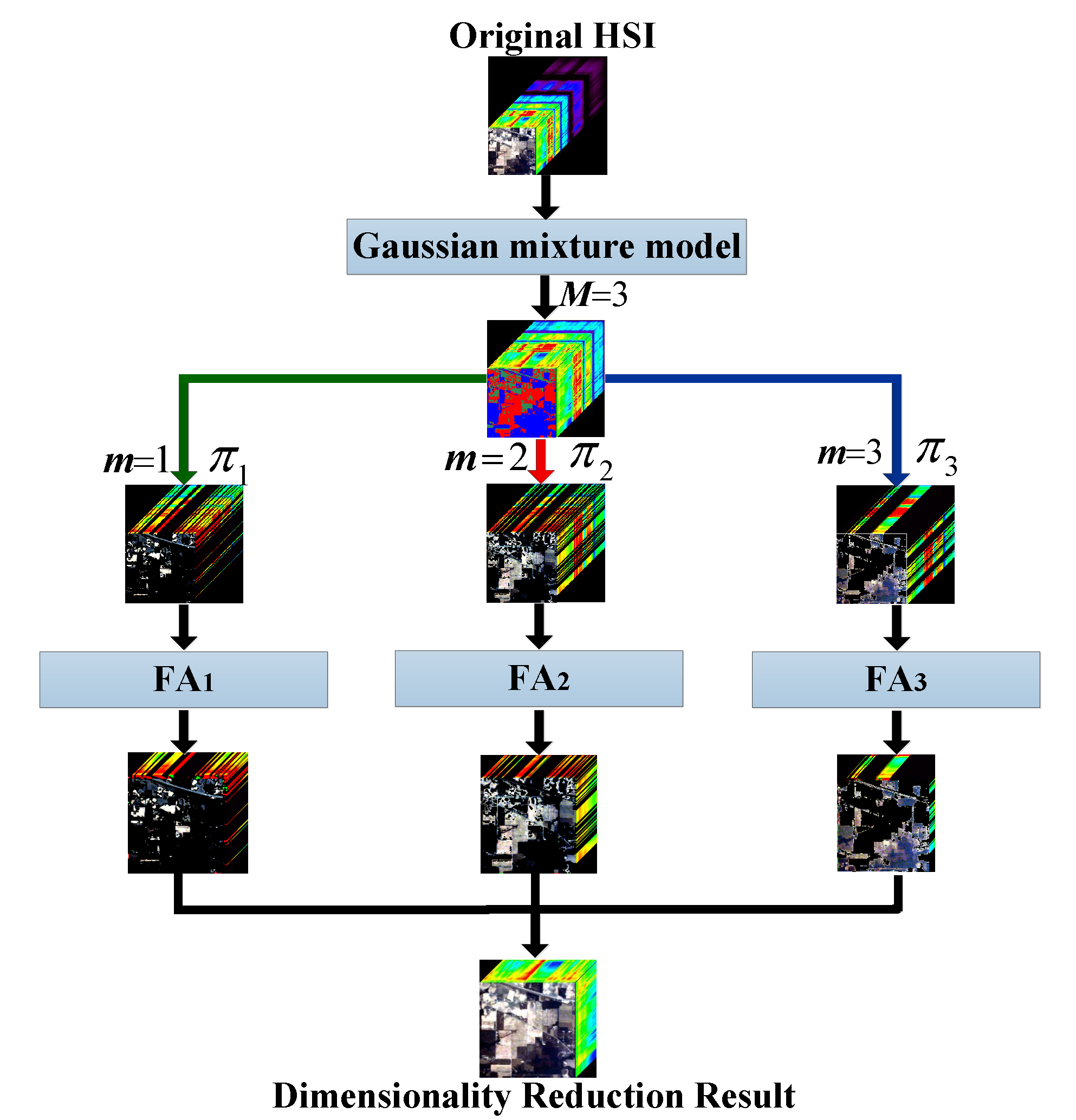
• An image segmentation method based on the Gaussian mixture model is proposed for MFA, DMFA, and SMFA to solve the problem of a non-normal distribution.
• Frameworks for extracting the most useful features for HSI classification based on the MFA, DMFA, and SMFA DR methods are proposed.

The paper is organized as follows. Section 2 briefly describes the three FE methods and a framework which automatically extracts optimal features for HSI classification. Section 3 presents experimental results and analysis of the results. Finally, Section 4 concludes the paper.

2. Proposed FE Methods and Framework

2.1. MFA

Let $\mathbf{x}$ denote a D-dimensional spectral vector, $\mathbf{z}$ denote a d-dimensional latent vector, and $m\in \{1,...,M\}$ denote the component indicator variable of the M factor analyzers in MFA. The MFA model can be defined as

$$p\left(m\right)={\pi }_m,\sum _{m=1}^M{\pi }_m=1,$$

(1)

$$p\left(\mathbf{z}\right|m)=p(\mathbf{z})=\mathcal{N}(\mathbf{z};\mathbf{0},\mathbf{I}),$$

(2)

$$p\left(\mathbf{x}\right|\mathbf{z},m)=\mathcal{N}(\mathbf{x};{\mathbf{W}}_m\mathbf{z}+{\mathsf{\mu }}_m,\mathsf{\Psi }),$$

(3)

where $\mathcal{N}(\mathbf{z};\mathbf{0},\mathbf{I})$ means that $\mathbf{z}$ is Gaussian vector with zero mean and $d\times d$ identity matrix $\mathbf{I}$ as the covariance matrix. The parameters of the m-th factor analyzer include a mixing proportion ${\pi }_m$, mean ${\mathsf{\mu }}_m$, a $D\times d$ factor loading matrix ${\mathbf{W}}_m$, and a $D\times D$ diagonal matrix $\mathsf{\Psi }$ which represents the independent noise variances for each band.

The parameters $\mathbf{z}$, ${\mathsf{\mu }}_m$, ${\mathbf{W}}_m$, and $\mathsf{\Psi }$ of MFA are estimated (trained) by using an expectation maximization (EM) algorithm [55]. An example demonstrating how MFA works is shown in Figure 1a,b. The schematic of the MFA is shown in Figure 2.

The performance of MFA for classification can be improved by increasing the dimensionality d of the latent factors per component of the mixture of factor analyzers or the number M of mixture components. However, for high dimensionality data, this approach quickly leads to overfitting. Below we discuss a cross-validation scheme to select d while avoiding overfitting.

2.2. DMFA

Figure 1c shows a case where the posteriors have non-normal distribution, to solve this problem the DMFA model was proposed. Instead of a simple standard normal prior, the DMFA model uses a more powerful MFA prior:

$$p\left(\mathbf{z}\right|m)=\mathrm{MFA}\left({\theta }_m^{\left(2\right)}\right),$$

(4)

where ${\theta }_m^{\left(2\right)}$ is the model parameter in the second layer and it emphasizes that the new MFA’s parameters are at the second layer and specific to component m of the first layer MFA, while holding the first layer parameters fixed. Thus, the DMFA is equivalent to fitting component-specific second layer MFAs with vectors drawn from $p(\mathbf{z},m,|\mathbf{x};{\theta }_m^{\left(1\right)})$ as data, where ${\theta }_m^{\left(1\right)}$ is the model parameter in the first layer.

Using $p\left(k_m\right|m)={\pi }_{k_m}^{\left(2\right)}$ to denote the second layer mixing proportion of mixture component $k_m$, and $K_m$ denote the total number of factor analyzers in the second layer for specific m of the first layer, so

$$\forall m:\sum _{k_m=1}^{K_m}{\pi }_{k_m}^{\left(2\right)}=1,$$

(5)

$$p_{DMFA}(\mathbf{z},m)=p\left(m\right)p\left(\mathbf{z}\right|m)=p\left(m\right)p\left(k_m\right|m)p\left(\mathbf{z}\right|k_m).$$

(6)

For convenience, denote all possible second layer mixture components with $s=1,...,S$, where $S={\sum }_{m=1}^M{K}_m$. The mixing proportions are ${\pi }_s^{\left(2\right)}=p\left(m\left(s\right)\right)p\left(k_m\left(s\right)\right|m\left(s\right))$, where $m\left(s\right)$ and $k_m\left(s\right)$ are the first and second layer mixture components m and $k_m$ to which s corresponds.

Therefore, the DMFA model is

$$p\left(s\right)={\pi }_s^{\left(2\right)},$$

(7)

$$p\left({\mathbf{z}}^{\left(2\right)}\right|s)=\mathcal{N}({\mathbf{z}}^{\left(2\right)};0,\mathbf{I}),$$

(8)

$$p\left({\mathbf{z}}^{\left(1\right)}\right|{\mathbf{z}}^{\left(2\right)},s)=\mathcal{N}({\mathbf{z}}^{\left(1\right)};{\mathbf{W}}_s^{\left(2\right)}{\mathbf{z}}^{\left(2\right)}+{\mathsf{\mu }}_s^{\left(2\right)},{\mathsf{\Psi }}^{\left(2\right)}),$$

(9)

$$m\leftarrow m\left(s\right),\left(\mathrm{deterministic}\right),$$

(10)

$$p\left(\mathbf{x}\right|{\mathbf{z}}^{\left(1\right)},m)=\mathcal{N}(\mathbf{x};{\mathbf{W}}_m^{\left(1\right)}{\mathbf{z}}^{\left(1\right)}+{\mathsf{\mu }}_m^{\left(1\right)},{\mathsf{\Psi }}^{\left(1\right)}),$$

(11)

where (10) is fully deterministic as each s belongs to one and only one m. ${\mathbf{z}}^{\left(1\right)}\in {\mathrm{R}}^{d^{\left(1\right)}}$, ${\mathbf{z}}^{\left(2\right)}\in {\mathrm{R}}^{d^{\left(2\right)}}$, ${\mathbf{W}}_m^{\left(1\right)}\in {\mathrm{R}}^{D\times d^{\left(1\right)}}$, ${\mathbf{W}}_s^{\left(2\right)}\in {\mathrm{R}}^{d^{\left(1\right)}\times d^{\left(2\right)}}$, ${\mathsf{\mu }}_m^{\left(1\right)}\in {\mathrm{R}}^{d^{\left(1\right)}}$, ${\mathsf{\mu }}_s^{\left(2\right)}\in {\mathrm{R}}^{d^{\left(2\right)}}$, ${\mathsf{\Psi }}^{\left(1\right)}$ and ${\mathsf{\Psi }}^{\left(2\right)}$ are $D\times D$ and $d^{\left(1\right)}\times d^{\left(1\right)}$ diagonal matrices of the first and second layers, respectively.

For the DMFA algorithm, the same scheme can be extended to training third-layer MFAs, but in this paper, we only consider the two-layer DMFA model.

The DMFA model can be trained by using a greedy layers-wise algorithm. The first layer of DMFA is trained as described above in Section 2.1, when training the second layer of DMFA, freezing the first layer parameters and treating the sampled first layer factor values for each mixture component ${\left\{{\mathbf{z}}_n^{\left(1\right)}\right\}}_m$ as training data for the second layer of DMFA. The DMFA model is summarized in Algorithm 1, and an illustration of the DMFA are shown in Figure 1c and Figure 3, respectively.

Algorithm 1 DMFA algorithm

Step 1: Input HSI $\mathbf{X}=\{{\mathbf{x}}_1,{\mathbf{x}}_2,...,{\mathbf{x}}_N\}$, the maximum number of EM iteration (default=1000).    Step 2: Train the first layer of DMFA on $\mathbf{X}$ with M mixture components and $d^{\left(1\right)}$ dimensional latent factors using the EM algorithm.   Step 3: Use the first layer latent factor dataset $Y_m={\left\{{\mathbf{z}}_n^{\left(1\right)}\right\}}_m$ for each of the M mixture components as training data for the second layer of DMFA.   Step 4: Train the second layer of DMFA on $Y_m$ with $d^{\left(2\right)}$ dimensional latent factors and $K_m$ mixture components using the EM algorithm.   Step 5: Output DR results $\mathbf{Z}=\{{\mathbf{z}}_1^{\left(2\right)},{\mathbf{z}}_2^{\left(2\right)},...,{\mathbf{z}}_N^{\left(2\right)}\}$.

2.3. SMFA

SMFA is a supervised FE method, let y denote an output value (label) for each D-dimensional labeled spectral vector $\mathbf{x}$. The SMFA model can be defined as

$$p\left(\mathbf{x}\right|\mathbf{z},m)=\mathcal{N}(\mathbf{x};{\mathbf{W}}_m\mathbf{z}+{\mathsf{\mu }}_m,\mathsf{\Psi }),$$

(12)

$$p\left(y\right|\mathbf{z},m)=\mathcal{N}(y;{\mathbf{W}}_{ym}\mathbf{z}+{\mathsf{\mu }}_{ym},{\mathsf{\Psi }}_y),$$

(13)

where the parameters of the m-th factor analyzer include mean ${\mathsf{\mu }}_m$, a $D\times d$ factor loading matrix ${\mathbf{W}}_m$, and a $D\times D$ diagonal matrix $\mathsf{\Psi }$ which represents the independent noise variances for each band. ${\mathbf{W}}_{ym}$, ${\mathsf{\mu }}_{ym}$, and ${\mathsf{\Psi }}_y$ are similar defined.

The parameters $\mathbf{z}$, ${\mathsf{\mu }}_m$, ${\mathbf{W}}_m$, $\mathsf{\Psi }$, ${\mathbf{W}}_{ym}$, ${\mathsf{\mu }}_{ym}$, and ${\mathsf{\Psi }}_y$ of SMFA are also estimated by using the EM algorithm [55]. The schematic of the SMFA is shown in Figure 4.

2.4. Framework

Traditionally, in DR, the dimensionality of desired features has to be initialized by the user. In this paper, we propose a framework that automatically selects the optimal dimensionality of desired features for HSI. We use the classification accuracy of a classifier on validation samples to automatically determine the dimensionality of the features. Different classifiers such as maximum likelihood (ML), support vector machine (SVM), and random forest (RF), can be used in this framework. The framework based on MFA, SMFA, and DMFA for HSI classification are summarized in Algorithms 2 and 3, respectively.

Algorithm 2 Framework based on MFA and SMFA

Step 1: Input HSI $\mathbf{X}$, training samples;    Step 2: Automatically select the optimal number of features d and mixture components M:          for $M=2:Mc$                for $d=3:\frac{D}{2}$                      Run MFA (or SMFA);                      Five-fold cross-validation of SVM (ML, or RF) on training samples;                      Save the cross-validation (CV) score ${\mathrm{CV}}_{M,d}$;                end          end          Return $\widehat{M}$ and $\widehat{d}$ corresponding to the best CV; Step 3: Run MFA (or SMFA) with $\widehat{M}$ and $\widehat{d}$;   Step 4: Run SVM (ML or RF) classification;   Step 5: Output Classification results.

Algorithm 3 Framework based on DMFA

Step 1: Input HSI $\mathbf{X}$, training samples;    Step 2: Automatically select the optimal number of features in the first layer $d^{\left(1\right)}$, in the second layer $d^{\left(2\right)}$, mixture components in the first layer M, and in the second layer $K_m$:          for $M=2:Mc$                for $d_1=3:\frac{D}{2}$                      for $K_m=2:M$                            for $d_2=3:d_1$                                  Run DMFA;                                  Five-fold cross-validation of SVM (ML, or RF) on training samples;                                  Save the cross-validation accuracy (CVA) ${\mathrm{CVA}}_{M,d_1,K_m,d_2}$;                            end                      end                end          end          Return $\widehat{M}$, $\widehat{d_1}$, $\widehat{K_m}$, and $\widehat{d_2}$ according to the best CVA; Step 3: Run DMFA with $M=\widehat{M}$, $d^{\left(1\right)}=\widehat{d_1}$, $K_m=\widehat{K_m}$, and $d^{\left(2\right)}=\widehat{d_2}$;   Step 4: Run SVM (ML or RF) classification;   Step 5: Output Classification results.

3. Experiments and Results

The experiments were done using ML, RF, and SVM classifiers, but since ML and RF gave inferior or slightly inferior results compared to SVM results, only the results of the SVM classifier are reported.

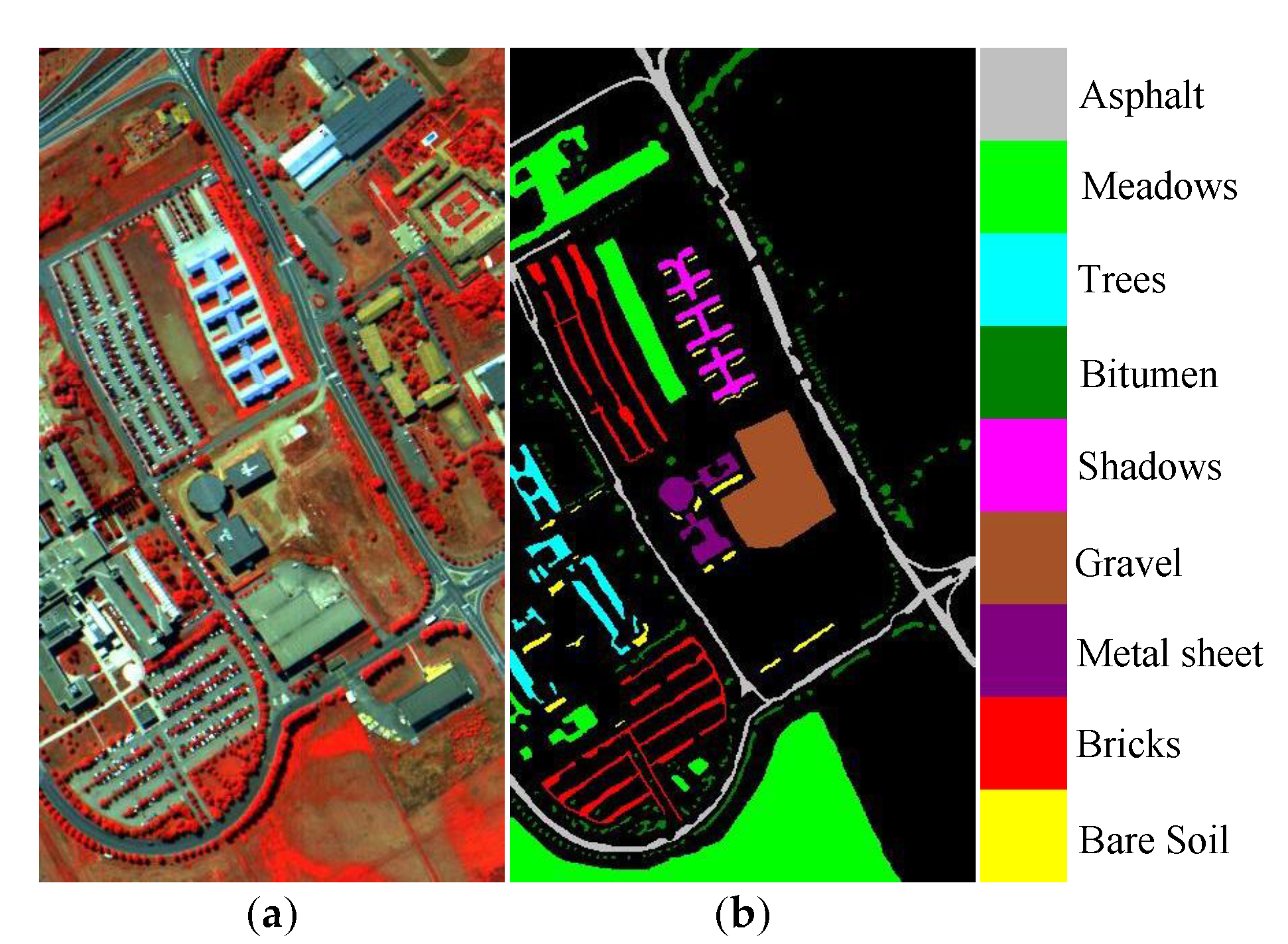
3.1. Experimental Datasets

The Indian Pines dataset was collected by the Airborne Visible/Infrared Imaging Spectrometer (AVIRIS) sensor at Indian Pines. The image contains $145\times 145$ pixels with a spatial resolution of 20 m and 220 spectral bands from 400 nm to 2500 nm. In the experiments, noisy bands and atmospheric vapor absorption bands are excluded leaving 200 spectral bands. Figure 5 shows the false-color composite of the Indian Pines image and the corresponding ground reference map, respectively. The nine largest classes are considered for classification [24,56]. For the Indian Pines, the University of Pavia, and the Salinas datasets, 10% of the labeled samples for each class are randomly selected as training samples, and the remaining 90% are used as the test set, respectively.

Table 1. Indian Pines HSI: Number of training and test samples.

$\mathbf{Class}\mathbf{Number}$	$\mathbf{Class}\mathbf{Name}$	$\mathbf{Training}\mathbf{Samples}$	$\mathbf{Test}\mathbf{Samples}$
1	Corn-no till	143	1291
2	Corn-min till	83	751
3	Grass/Pasture	50	447
4	Grass/Trees	75	672
5	Hay-windrowed	49	440
6	Soybean-no till	97	871
7	Soybean-min till	247	2221
8	Soybean-clean till	61	553
9	Woods	129	1165
	Total	934	8411

,

Table 2. University of Pavia dataset: Number of training and test samples.

$\mathbf{Class}\mathbf{Number}$	$\mathbf{Class}\mathbf{Name}$	$\mathbf{Training}\mathbf{Samples}$	$\mathbf{Test}\mathbf{Samples}$
1	Asphalt	663	5968
2	Meadows	1865	16,784
3	Gravel	210	1889
4	Trees	306	2758
5	Painted metal sheets	135	1210
6	Bare Soil	503	4526
7	Bitumen	133	1197
8	Self-Blocking Bricks	368	3314
9	Shadows	95	852
	Total	4278	38,498

and

Table 3. Salinas dataset: Number of training and test samples.

$\mathbf{Class}\mathbf{Number}$	$\mathbf{Class}\mathbf{Name}$	$\mathbf{Training}\mathbf{Samples}$	$\mathbf{Test}\mathbf{Samples}$
1	Brocoli_green_weeds_1	201	1808
2	Brocoli_green_weeds_2	373	3353
3	Fallow	198	1778
4	Fallow_rough_plow	139	1255
5	Fallow_smooth	268	2410
6	Stubble	396	3563
7	Celery	358	3221
8	Grapes_untrained	1127	10,144
9	Soil_vinyard_develop	620	5583
10	Corn_senesced_green_weeds	328	2950
11	Lettuce_romaine_4wk	107	961
12	Lettuce_romaine_5wk	193	1734
13	Lettuce_romaine_6wk	92	824
14	Lettuce_romaine_7wk	107	963
15	Vinyard_untrained	727	6541
16	Vinyard_vertical_trellis	181	1626
	Total	5415	48,714

provide information on the number of training and test samples for each class of interest, respectively.

The Houston dataset was provided by the IEEE Geoscience and Remote Sensing Society (GRSS) for the Data Fusion Contest in 2013. This image is of the University of Houston campus and the neighboring urban area. The dataset has $349\times 1905$ pixels with a spatial resolution of 2.5 m and 114 spectral bands coverage ranging from 380 nm to 1050 nm. This HSI contains fifteen classes of interest. Figure 6 shows the false-color composite of the Houston image and the corresponding ground reference map, respectively. The training and test samples were given according to the IEEE GRSS Data Fusion Contest in 2013. The spatial positions and the number of training and test samples for each class of interest is fixed by the IEEE GRSS Data Fusion Contest.

Table 4. Houston dataset: Number of training and test samples.

$\mathbf{Class}\mathbf{Number}$	$\mathbf{Class}\mathbf{Name}$	$\mathbf{Training}\mathbf{Samples}$	$\mathbf{Test}\mathbf{Samples}$
1	Healthy grass	198	1053
2	Stressed grass	190	1064
3	Synthetic grass	192	505
4	Trees	188	1056
5	Soil	186	1056
6	Water	182	143
7	Residential	196	1072
8	Commercial	191	1053
9	Road	193	1059
10	Highway	191	1036
11	Railway	181	1054
12	Parking Lot 1	192	1041
13	Parking Lot 2	184	285
14	Tennis Court	181	247
15	Running Track	187	473
	Total	2832	12,197

provides information on the number of training and test samples for each class of interest. It is important to note that the standard sets of training and test samples were used for the dataset to make the results entirely comparable with most of the methods available in the literature.

The University of Pavia dataset was captured by the Reflective Optics System Imaging Spectrometer sensor over the city of Pavia, Italy. This image has $610\times 340$ pixels with a spatial resolution of 1.3 m and 115 spectral bands coverage ranging from 0.43 $\mathsf{\mu }$m to 0.86 $\mathsf{\mu }$m. In the experiments, this data contains nine classes of interest and has 103 spectral bands after removing 12 noisy bands. Figure 7 shows the false-color composite of the University of Pavia image and the corresponding ground reference map.

The Salinas dataset was acquired by the AVIRIS sensor over Salinas Valley, California. This image has $512\times 217$ pixels with a spatial resolution of 3.7 m and 204 spectral bands after removing 20 water absorption bands. This image contains sixteen classes of interest. Figure 8 shows the false-color composite of the Salinas image and the corresponding ground reference map.

3.2. Experimental Setup

An SVM classifier is used to evaluate the performance of the proposed methods. The SVM classifier is a supervised classification method that uses a kernel method to map the data with a non-linear transformation to a higher dimensional space and in that space tries to find a linear separating hyperplane from different classes. In the experiments, for SVM, the LibSVM Toolbox for MATLAB was applied with a radial basis function (RBF) kernel [57,58]. The five-fold cross-validation is used to find the best parameters, i.e., the kernel parameter and regularization parameter, in SVM. The evaluation metrics used are overall accuracy (OA), average accuracy (AA), and Kappa coefficient (KC), as well as standard deviation (STD). To further evaluate the performance of the proposed algorithms, the following statistical and DR methods: PCA, PPCA, FA, LDA, NWFE, MFA, DMFA, and SMFA are used for comparison. Each experiment is run ten times, and the average of these ten experiments is reported.

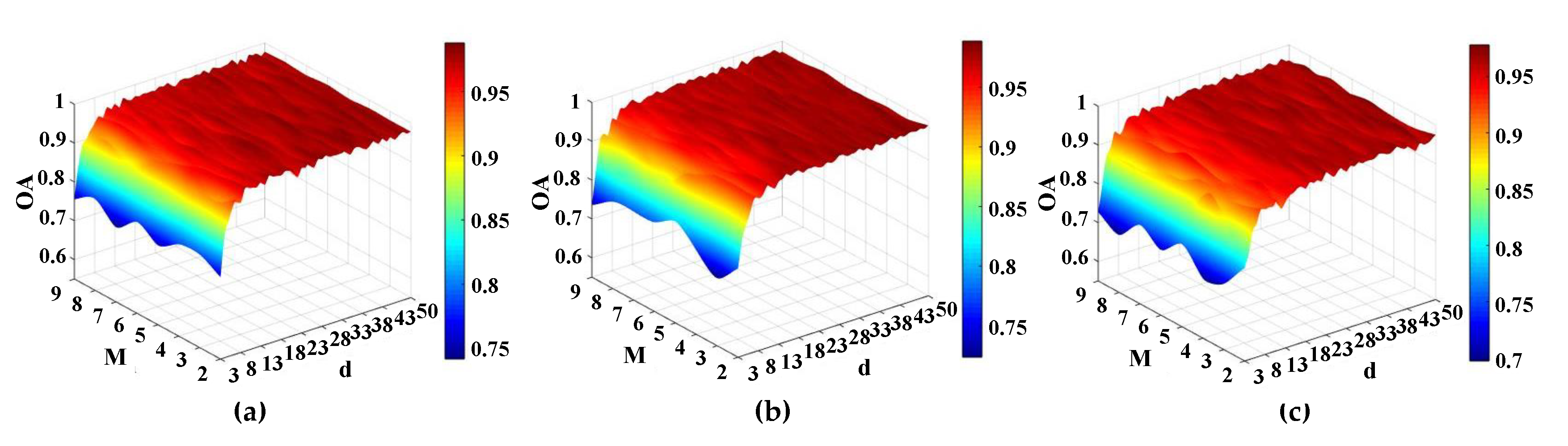
3.3. Tuning Parameter Estimation and Assessment

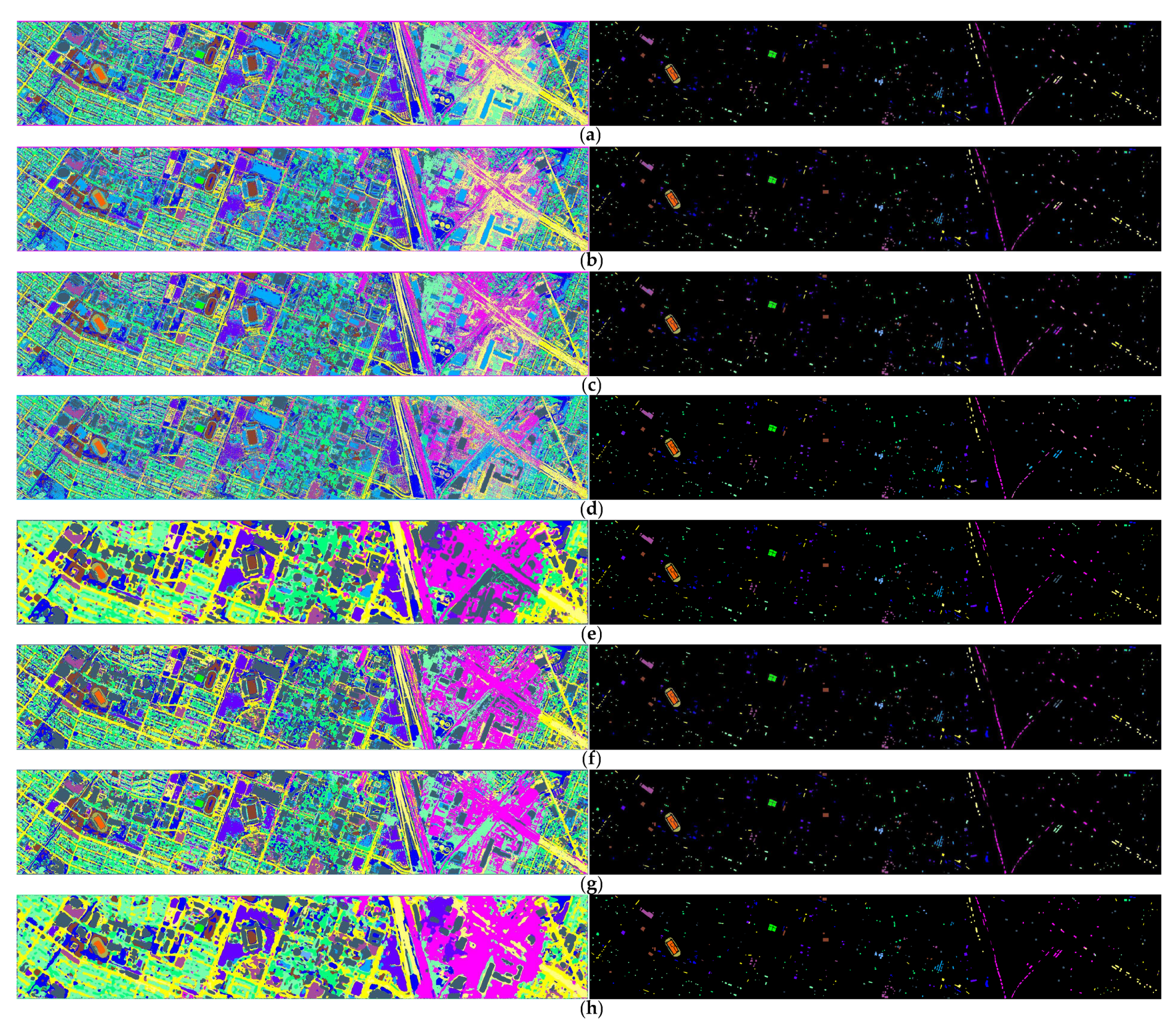
For the MFA and SMFA algorithms, we need to estimate the number of mixture components M, and the dimensionality of latent factors d. In the experiments, $M\in \{2,3,...,Mc\}$, where $Mc$ is the maximal number of classes considered, $d\in \{3,4,...,D/2\}$, where D is the input dimensionality of original datasets, we use five-fold cross-validation to obtain the optimal parameters M and d.

The assessment of the effect of the tuning parameters (M and d) on the performance of the proposed methods was of interest. Since we were interested in the classification accuracy, we investigated the effect of the number of mixture components M and the dimensionality of latent factors d on OA. Figure 9a,b shows the 3-dimensional surface of the OA of MFA and SMFA with respect to the values of parameters M and d for the SVM classifier, respectively. It can be seen that the OA gradually increases in the beginning as the d increases, and then keeps stable with slight fluctuation as the d increases, but decreases slightly when the d reaches some value. It can also be observed that the OA is insensitive to M.

For the DMFA algorithm, we need to estimate the number of mixture components M and $K_m$, and the dimensionality of latent factors $d^{\left(1\right)}$ and $d^{\left(2\right)}$, in the first and second layer of DMFA, respectively. In the experiments, M is the same as in the MFA, $K_m\in \{2,...,M\}$, we set $K_m=2$ for all m in our experiments. $d^{\left(1\right)}$ is the same as d, $d^{\left(2\right)}\in \{3,4,...,d^{\left(1\right)}\}$. Five-fold cross-validation can be used to obtain the optimal parameters. To analyze the impact of the number of mixture components M and the dimensionality of latent factors $d^{\left(1\right)}$ in the first layer on the performance of DMFA, the output results of the first layer of DMFA were used for HSI classification. Figure 9c shows the OAs with respect to the values of parameters M and $d^{\left(1\right)}$. Figure 9a,b show similar things for MFA and SMFA, respectively.

3.4. Classification

The first experiment was performed on the Indian Pines dataset. Figure 10 shows the classification maps obtained by different methods. From the figures, it can be seen that the classification maps obtained by PCA, PPCA, FA, LDA, and NWFE are not very satisfactory since they have lots of visible noise. By contrast, MFA, DMFA, and SMFA give much better classification maps, all of them have a smoother appearance and preserve more details on edges. Besides visual comparison,

Table 5. The classification results (%) of different DR methods on the Indian Pines dataset, the best results are in bold typeface. The row of each class number (CN) is the mean accuracy ± standard deviation based on ten runs. The best classification results are given in bold typeface.

$\mathbf{CN}$	$\mathbf{PCA}$	$\mathbf{PPCA}$	$\mathbf{FA}$	$\mathbf{LDA}$	$\mathbf{NWFE}$	$\mathbf{MFA}$	$\mathbf{DMFA}$	$\mathbf{SMFA}$
1	75.13 ± 2.39	81.22 ± 1.39	86.48 ± 1.93	89.31 ± 0.98	84.51 ± 2.25	93.00 ± 1.87	97.49 ± 1.51	96.34 ± 1.32
2	83.33 ± 2.16	84.00 ± 4.21	89.30 ± 3.49	72.44 ± 3.97	82.82 ± 2.16	91.71 ± 1.05	99.17 ± 0.89	95.61 ± 1.04
3	94.51 ± 1.62	94.77 ± 2.27	97.48 ± 0.89	92.84 ± 2.62	91.50 ± 1.75	94.42 ± 1.08	97.35 ± 1.66	95.08 ± 1.51
4	96.09 ± 1.02	95.95 ± 0.99	97.65 ± 0.98	97.32 ± 1.62	98.51 ± 1.49	98.53 ± 0.40	98.39 ± 0.47	98.81 ± 1.08
5	99.55 ± 0.14	99.77 ± 0.18	99.84 ± 0.16	99.55 ± 0.23	99.32 ± 0.16	99.83 ± 0.18	99.86 ± 0.14	99.84 ± 0.18
6	75.03 ± 1.99	82.06 ± 2.27	82.50 ± 2.14	80.37 ± 2.89	82.43 ± 3.00	90.53 ± 0.68	95.48 ± 1.40	97.36 ± 0.62
7	78.22 ± 1.85	77.62 ± 1.45	88.40 ± 1.70	82.85 ± 2.05	88.74 ± 2.11	95.56 ± 1.58	96.91 ± 1.22	98.24 ± 1.42
8	83.54 ± 2.68	83.00 ± 2.34	89.21 ± 2.68	77.76 ± 2.74	79.57 ± 3.56	96.75 ± 1.34	98.74 ± 1.03	99.28 ± 1.06
9	99.40 ± 0.32	99.83 ± 0.41	99.66 ± 0.26	99.57 ± 0.36	99.49 ± 0.55	99.83 ± 0.30	99.74 ± 0.54	99.91 ± 0.46
AA	87.20 ± 0.35	88.69 ± 0.73	92.30 ± 0.67	88.00 ± 0.64	89.65 ± 0.88	95.59 ± 1.01	98.14 ± 0.86	97.85 ± 0.51
OA	84.48 ± 0.35	85.98 ± 0.39	90.96 ± 0.60	87.20 ± 0.56	89.28 ± 0.82	95.59 ± 0.86	97.86 ± 0.72	97.90 ± 0.60
KC	0.8173 ± 0.0040	0.8345 ± 0.0048	0.8940 ± 0.0072	0.8495 ± 0.0065	0.8738 ± 0.0096	0.9459 ± 0.0102	0.9749 ± 0.0085	0.9753 ± 0.0070

presents the quantitative classification results for all the methods, and there it can be observed that the MFA, DMFA, and SMFA achieve much higher classification accuracies than PCA, PPCA, and FA, respectively. These results imply that the performance of DR could be improved by considering the Gaussian mixture model. Moreover, DMFA and SMFA clearly outperform MFA, and the performance of DMFA and SMFA is similar, both of them present the highest OA, AA, and KC and achieves most of the top classification accuracy values for individual classes. This indicates that MFA, DMFA, and SMFA could extract more useful information for classification from a complicated HSI. Moreover, SMFA is better than LDA and NWFE, this means that SMFA is an effective supervised DR method. MFA, DMFA, and SMFA improve the OA by 11.11%, 13.38%, and 13.42% using SVM compared to other methods in the experiment, respectively. It is interesting to note that all DR methods based on FA (SMFA, DMFA, MFA, and FA) gave a better performance than PCA and PPCA. The reason for this is that noise could be distributed inconsistently for different components in real HSI. Table 5 also gives the STDs of classification results for different DR methods for the Indian Pines dataset. It can be seen that all the methods give similar and stable classification results.

Table 6. CPU processing times in seconds by different DR methods applied to the Indian Pines (INPS), Houston (HSN), University of Pavia (UPA), and Salinas (SAS) datasets (the number of features = 20).

Datasets	PCA	PPCA	FA	LDA	NWFE	MFA	DMFA	SMFA
INPS	0.11	63.66	70.89	0.12	1.05	3.85	18.07	0.12
HSN	2.91	1335.09	21.45	0.89	5.02	103.77	151.91	4.54
UPA	0.62	285.01	4.01	0.21	0.91	28.10	79.30	1.55
SAS	0.56	356.44	22.15	0.38	−	18.97	87.85	1.62

compares the CPU processing time (in seconds) used by different DR methods for the Indian Pines dataset. All methods were implemented in Matlab R2019a on a computer having Intel(R) Core(TM) i7-6700 processor (3.40 GHz), 8.00 GB of memory, and 64-bit Windows 10 Operating System. It can be seen that the running times for MFA, DMFA, and SMFA were 3.85, 18.07, and 0.12 s, respectively. It is worth noting that the running time for the supervised methods (LDA, NWFE, and SMFA) is affected considerably by the number of labeled (training) samples used, and the unsupervised methods are affected by the total size of the dataset.

The second experiment was performed on the Houston dataset. Figure 11 shows the classification maps obtained by different methods. From the figures, we can see that the proposed MFA, DMFA, and SMFA algorithms also outperform the other algorithms.

Table 7. The classification results (%) of different DR methods on the Houston dataset, the best results are in bold typeface. The row of each class number (CN) is the mean accuracy ± standard deviation based on ten runs.

$\mathbf{CN}$	$\mathbf{PCA}$	$\mathbf{PPCA}$	$\mathbf{FA}$	$\mathbf{LDA}$	$\mathbf{NWFE}$	$\mathbf{MFA}$	$\mathbf{DMFA}$	$\mathbf{SMFA}$
1	98.05	96.20 ± 0.29	96.37	80.53	80.72 ± 0.45	98.98 ± 0.89	99.31 ± 1.66	79.49 ± 1.37
2	96.01	96.36 ± 0.13	95.97	80.92	82.99 ± 0.18	95.33 ± 1.63	95.24 ± 1.58	83.46 ± 1.57
3	100	99.97 ± 0.27	100	100	99.42 ± 0.58	99.76 ± 0.24	99.82 ± 0.19	99.48 ± 0.34
4	98.05	97.35 ± 1.36	97.72	92.90	89.49 ± 0.94	99.89 ± 0.32	99.47 ± 1.78	89.30 ± 2.09
5	97.41	97.45 ± 0.16	97.11	96.97	98.86 ± 0.38	98.42 ± 0.82	98.11 ± 1.09	99.96 ± 0.11
6	99.94	95.07 ± 0.46	95.30	93.71	95.11 ± 0.21	47.24 ± 0.80	99.97 ± 0.27	92.31 ± 0.35
7	81.34	82.05 ± 0.31	87.91	84.80	79.76 ± 2.44	66.22 ± 1.38	89.53 ± 3.02	82.37 ± 1.23
8	81.45	68.87 ± 0.17	84.18	71.13	72.46 ± 4.73	84.06 ± 1.14	81.82 ± 2.64	90.03 ± 0.11
9	83.40	78.34 ± 0.60	78.08	72.52	75.54 ± 1.19	87.65 ± 1.04	91.66 ± 0.66	83.95 ± 1.08
10	70.03	83.58 ± 0.48	65.32	73.17	81.27 ± 3.21	86.21 ± 0.24	66.67 ± 4.76	97.97 ± 1.59
11	67.86	69.57 ± 1.86	57.04	85.39	93.55 ± 2.10	68.21 ± 0.16	74.51 ± 0.59	88.99 ± 4.01
12	85.50	89.15 ± 5.12	82.68	82.52	85.11 ± 1.86	95.80 ± 2.28	94.07 ± 2.64	96.25 ± 1.19
13	30.69	30.06 ± 1.33	43.85	70.53	70.88 ± 1.74	92.52 ± 3.26	89.56 ± 2.31	65.26 ± 0.89
14	99.18	98.39 ± 0.24	89.05	99.19	99.60 ± 0.31	94.64 ± 0.83	97.24 ± 1.13	99.96 ± 0.22
15	100	99.41 ± 0.59	100	95.98	98.73 ± 0.50	99.54 ± 0.54	99.88 ± 0.14	91.97 ± 1.61
AA	85.93	85.50 ± 0.50	84.70	85.35	86.94 ± 0.47	87.68 ± 0.36	91.81 ± 0.39	89.42 ± 0.69
OA	83.45	83.75 ± 0.59	82.05	83.59	85.35 ± 0.56	86.65 ± 0.42	88.72 ± 0.49	89.40 ± 0.67
KC	0.8207	0.8240 ± 0.0065	0.8053	0.8223	0.8412 ± 0.0059	0.8552 ± 0.0046	0.8775 ± 0.0053	0.8848 ± 0.0075

presents the quantitative classification results of the different DR methods. As shown in Table 7, the performance of DMFA and SMFA is better than MFA and much better than PCA, PPCA, FA, LDA, and NWFE. MFA, DMFA, and SMFA improve the OA by 4.60%, 6.67%, and 7.35% compared to other methods in the experiment, respectively. Table 7 also presents the STDs of classification results. It can be seen that FA and LDA present the most stable results. MFA, DMFA, and SMFA have slight fluctuation for each experiment and give relatively stable results.

The third and fourth experiments were performed on the University of Pavia and Salinas datasets. It should be noted that the NWFE method does not work for the Salinas dataset. Therefore, in the experiments of the Salinas dataset, there are no experimental results for NWFE. Figure 12 and Figure 13 show the classification maps obtained by different methods on the University of Pavia and Salinas datasets, respectively. From Figure 12 and Figure 13, it can be seen that the classification maps obtained by MFA, DMFA, and SMFA are much better than PCA, PPCA, FA, LDA, and NWFE, respectively.

Table 8. The classification results (%) of different DR methods on the University of Pavia dataset, the best results are in bold typeface. The row of each class number (CN) is the mean accuracy ± standard deviation based on ten runs.

$\mathbf{CN}$	$\mathbf{PCA}$	$\mathbf{PPCA}$	$\mathbf{FA}$	$\mathbf{LDA}$	$\mathbf{NWFE}$	$\mathbf{MFA}$	$\mathbf{DMFA}$	$\mathbf{SMFA}$
1	92.00 ± 1.01	93.16 ± 0.82	94.65 ± 0.58	93.20 ± 0.55	94.10 ± 0.49	98.07 ± 0.45	98.39 ± 0.66	98.69 ± 0.27
2	95.71 ± 0.53	96.12 ± 0.25	96.43 ± 0.24	96.86 ± 0.41	97.52 ± 0.38	99.68 ± 0.10	99.02 ± 0.42	99.79 ± 0.08
3	78.98 ± 2.06	82.23 ± 1.86	80.16 ± 1.72	76.13 ± 2.81	74.01 ± 4.00	90.15 ± 2.29	98.39 ± 1.44	94.28 ± 1.93
4	94.24 ± 0.95	94.61 ± 0.82	93.86 ± 0.78	92.57 ± 0.90	89.63 ± 1.26	95.65 ± 0.36	98.72 ± 0.95	96.27 ± 0.61
5	99.41 ± 2.27	98.99 ± 2.01	99.21 ± 1.23	99.17 ± 0.16	99.59 ± 0.13	99.89 ± 0.12	99.93± 0.35	99.81 ± 0.09
6	90.96 ± 2.01	91.80 ± 0.75	93.54 ± 1.09	81.11 ± 1.06	90.39 ± 1.72	98.63 ± 0.30	99.80 ± 0.88	99.98 ± 0.30
7	85.40 ± 4.34	88.69 ± 1.98	90.08 ± 2.19	80.95 ± 1.35	83.12 ± 4.17	94.32 ± 0.76	99.75 ± 1.06	99.92 ± 0.68
8	77.35 ± 2.14	83.85 ± 0.97	84.40 ± 1.61	86.33 ± 2.03	84.91 ± 2.30	94.63 ± 0.81	97.15 ± 1.12	97.31 ± 1.54
9	91.55 ± 1.78	99.89± 0.58	99.31± 0.87	99.65 ± 0.18	99.88 ± 0.11	97.07 ± 0.93	99.64 ± 1.07	97.77 ± 0.58
AA	89.57 ± 0.53	92.27 ± 0.39	92.57 ± 0.48	89.55 ± 0.19	90.35 ± 0.66	96.47 ± 0.30	98.98 ± 0.49	98.22 ± 0.25
OA	91.78 ± 0.29	93.32 ± 0.27	93.80 ± 0.29	91.85 ± 0.18	93.02 ± 0.32	97.90 ± 0.14	98.87 ± 0.41	98.87 ± 0.14
KC	0.8908 ± 0.0038	0.9112 ± 0.0036	0.9177 ± 0.0038	0.8314 ± 0.0023	0.9071 ± 0.0043	0.9722 ± 0.0019	0.9850 ± 0.0055	0.9850 ± 0.0019

and

Table 9. The classification results (%) of different DR methods on the Salinas dataset, the best results are in bold typeface. The row of each class number (CN) is the mean accuracy ± standard deviation based on ten runs.

$\mathbf{CN}$	$\mathbf{PCA}$	$\mathbf{PPCA}$	$\mathbf{FA}$	$\mathbf{LDA}$	$\mathbf{MFA}$	$\mathbf{DMFA}$	$\mathbf{SMFA}$
1	99.91± 0.17	99.32± 0.02	99.29± 0.38	99.95 ± 0.05	99.94± 0.09	99.82 ± 0.08	99.89± 0.18
2	99.88 ± 0.23	99.97 ± 0.09	99.82 ± 0.14	99.79 ± 0.03	99.79 ± 0.12	99.99± 0.21	99.99± 0.12
3	98.88 ± 0.36	99.04 ± 0.29	99.21 ± 0.16	99.78 ± 0.12	99.83 ± 0.07	99.72 ± 0.21	99.96± 0.22
4	99.13 ± 0.48	99.76 ± 0.42	99.76 ± 0.30	99.12 ± 0.53	98.96 ± 0.50	97.93 ± 0.46	98.41 ± 0.18
5	99.05 ± 0.64	98.19 ± 0.56	99.13 ± 0.15	98.96 ± 0.32	99.50 ± 0.34	99.92 ± 0.42	99.17 ± 0.20
6	99.94 ± 0.20	99.92± 0.09	99.03± 0.06	99.83 ± 0.08	99.23 ± 0.20	99.98± 0.14	99.97 ± 0.05
7	99.94 ± 0.19	99.89± 0.14	99.95± 0.20	99.94 ± 0.09	99.81 ± 0.10	99.91 ± 0.13	99.91 ± 0.12
8	88.88 ± 0.92	87.55 ± 1.01	84.53 ± 1.12	90.09 ± 1.29	97.73 ± 0.91	99.25 ± 0.04	99.71 ± 0.60
9	99.44 ± 0.16	99.38 ± 0.14	99.34 ± 0.15	99.95 ± 0.20	99.91 ± 0.07	99.93 ± 0.29	99.99± 0.03
10	96.27 ± 0.53	98.19 ± 0.72	97.80 ± 0.82	98.61 ± 0.45	98.99 ± 0.44	99.49 ± 0.83	99.76 ± 0.87
11	99.03 ± 0.80	99.04 ± 0.74	99.68 ± 0.47	98.86 ± 0.41	99.97 ± 0.19	99.90 ± 1.08	99.97± 0.28
12	98.36 ± 0.14	98.86 ± 0.07	99.26 ± 0.15	99.97± 0.32	99.94 ± 0.49	99.71 ± 0.15	99.89 ± 0.13
13	99.52 ± 0.51	99.76 ± 0.25	99.76 ± 0.22	99.39 ± 0.29	99.43± 0.09	99.52 ± 0.60	99.96± 0.45
14	99.79 ± 1.02	98.43 ± 0.83	99.16 ± 0.58	96.78 ± 0.93	99.93 ± 1.23	99.27 ± 1.60	99.99± 0.15
15	84.51 ± 1.20	85.68 ± 1.54	83.23 ± 1.96	72.62 ± 2.44	97.38 ± 1.15	98.03 ± 1.64	97.75 ± 2.26
16	99.38 ± 0.30	99.75 ± 0.74	99.58± 1.15	98.65 ± 0.44	99.76± 0.97	99.08 ± 0.63	99.92± 0.80
AA	97.62 ± 0.15	87.73 ± 0.12	97.54 ± 0.09	97.02 ± 0.12	99.49 ± 0.08	99.47 ± 0.26	99.66 ± 0.14
OA	95.09 ± 0.17	95.08 ± 0.09	94.19 ± 0.12	93.91 ± 0.10	99.02 ± 0.20	99.40 ± 0.40	99.53 ± 0.34
KC	0.9453 ± 0.0019	0.9452 ± 0.0010	0.9353 ± 0.0013	0.9321 ± 0.0011	0.9890 ± 0.0022	0.9933 ± 0.0045	0.9948 ± 0.0038

present the quantitative classification results. As shown in Table 8 and Table 9, the classification accuracies of the proposed MFA, DMFA, and SMFA methods are much better than PCA, PPCA, and FA methods. These results further demonstrate that, instead of using a single Gaussian distribution model, the performance of DR could be improved by considering the Gaussian mixture model. For the University of Pavia dataset, MFA, DMFA, and SMFA improve the OA by 6.05%, 7.02%, and 7.02% compared to other methods used in the experiment, respectively. For the Salinas dataset, MFA, DMFA, and SMFA improve the OA by 5.11%, 5.49%, and 5.62% compared to other methods used in the experiment, respectively. Moreover, in the experiments, DMFA and SMFA are clearly better than MFA, and DMFA and SMFA give similar and highest OA, AA, and KC and also achieve most of the top classification accuracy values for the individual classes. This also further indicates that MFA, DMFA, and SMFA could extract more effective information for classification from a complicated HSI. Table 8 and Table 9 also give the STDs of classification results for different DR methods for the University of Pavia and Salinas datasets, respectively. It can be seen that all the methods give similar and relatively stable classification results. This also further demonstrates that MFA, DMFA, and SMFA are stable and effective DR methods.

4. Conclusions

In this paper, MFA, DMFA, and SMFA were proposed for feature extraction of HSIs and were then used for classification of them. MFA, DMFA, and SMFA are probabilistic DR methods, instead of assuming that a whole HSI obeys a Gaussian distribution, the methods use a Gaussian mixture model to extract more effective information for DR. The Gaussian mixture model is used for MFA to allow a low-dimensionality representation of the Gaussian. A two-layer MFA, DMFA, utilizes the samples from the posterior at the first layer to an MFA model at the second layer. MFA and DMFA are two unsupervised DR method. The methods are particularly suitable for DR of HSI with a non-normal distribution and unlabeled samples. SMFA is a supervised DR method and uses labeled samples to extract features. SMFA can be effectively used to DR of HSI with a non-normal distribution and labeled samples.

Based on the three DR methods, we also proposed a framework for HSI classification, the overall accuracy of a classifier on validation samples is used to automatically determine the optimal number of features of DR for HSI classification. This framework can automatically extract the most effective feature for HSI classification. To validate the performance of DR, we conduct experiments in terms of SVM classification based on four real HSIs. The experimental results show that MFA, DMFA, and SMFA can give better results than statistical DR comparison methods.

In the future, more validations on other applications, e.g., hyperspectral unmixing, target detection, will be incorporated in our future work.

References

1. Harsanyi, J.C.; Chang, C.I. Hyperspectral image classification and dimensionality reduction: An orthogonal subspace projection approach. IEEE Trans. Geosci. Remote Sens. 1994, 32, 779–785. [Google Scholar] [CrossRef] [Green Version]
2. Jia, X.; Richards, J.A. Segmented principal components transformation for efficient hyperspectral remote-sensing image display and classification. IEEE Trans. Geosci. Remote Sens. 1999, 37, 538–542. [Google Scholar]
3. Camps-Valls, G.; Bruzzone, L. Kernel-based methods for hyperspectral image classification. IEEE Trans. Geosci. Remote Sens. 2005, 43, 1351–1362. [Google Scholar] [CrossRef]
4. Chen, Y.; Nasrabadi, N.M.; Tran, T.D. Hyperspectral image classification using dictionary-based sparse representation. IEEE Trans. Geosci. Remote Sens. 2011, 49, 3973–3985. [Google Scholar] [CrossRef]
5. Chang, C.; Du, Q.; Sun, T.; Althouse, M.L. A joint band prioritization and band-decorrelation approach to band selection for hyperspectral image classification. IEEE Trans. Geosci. Remote Sens. 1999, 37, 2631–2641. [Google Scholar] [CrossRef] [Green Version]
6. Feng, F.; Li, W.; Du, Q.; Zhang, B. Dimensionality reduction of hyperspectral image with graph-based discriminant analysis considering spectral similarity. Remote Sens. 2017, 9, 323. [Google Scholar] [CrossRef] [Green Version]
7. Xu, X.; Li, J.; Huang, X.; Dalla-Mura, M.; Plaza, A. Multiple morphological component analysis based decomposition for remote sensing image classification. IEEE Trans. Geosci. Remote Sens. 2016, 54, 3083–3102. [Google Scholar] [CrossRef]
8. Zhang, L.; Zhang, L.; Tao, D.; Huang, X. On combining multiple features for hyperspectral remote sensing image classification. IEEE Trans. Geosci. Remote Sens. 2011, 50, 879–893. [Google Scholar] [CrossRef]
9. Maxwell, A.E.; Warner, T.A.; Fang, F. Implementation of machine-learning classification in remote sensing: An applied review. Int. J. Remote Sens. 2018, 39, 2784–2817. [Google Scholar] [CrossRef] [Green Version]
10. Wieland, M.; Pittore, M. Performance evaluation of machine learning algorithms for urban pattern recognition from multi-spectral satellite images. Remote Sens. 2014, 6, 2912–2939. [Google Scholar] [CrossRef] [Green Version]
11. Pal, M.; Foody, G.M. Feature selection for classification of hyperspectral data by SVM. IEEE Trans. Geosci. Remote Sens. 2010, 48, 2297–2307. [Google Scholar] [CrossRef] [Green Version]
12. Hughes, G. On the mean accuracy of statistical pattern recognizers. IEEE Trans. Inf. Theory 1968, 14, 55–63. [Google Scholar] [CrossRef] [Green Version]
13. Melgani, F.; Bruzzone, L. Classification of hyperspectral remote sensing images with support vector machines. IEEE Trans. Geosci. Remote Sens. 2004, 42, 1778–1790. [Google Scholar] [CrossRef] [Green Version]
14. Zhang, L.; Zhong, Y.; Huang, B.; Gong, J.; Li, P. Dimensionality reduction based on clonal selection for hyperspectral imagery. IEEE Trans. Geosci. Remote Sens. 2007, 45, 4172–4186. [Google Scholar] [CrossRef]
15. Luo, F.; Huang, H.; Duan, Y.; Liu, J.; Liao, Y. Local geometric structure feature for dimensionality reduction of hyperspectral imagery. Remote Sens. 2017, 9, 790. [Google Scholar] [CrossRef] [Green Version]
16. Huang, H.; Yang, M. Dimensionality reduction of hyperspectral images with sparse discriminant embedding. IEEE Trans. Geosci. Remote Sens. 2015, 53, 5160–5169. [Google Scholar] [CrossRef]
17. Ulfarsson, M.O.; Palsson, F.; Sigurdsson, J.; Sveinsson, J.R. Classification of big data with application to imaging genetics. Proc. IEEE 2016, 104, 2137–2154. [Google Scholar] [CrossRef] [Green Version]
18. Gormus, E.T.; Canagarajah, N.; Achim, A. Dimensionality reduction of hyperspectral images using empirical mode decompositions and wavelets. IEEE J. Sel. Top. Appl. Earth Obs. Remote Sens. 2012, 5, 1821–1830. [Google Scholar] [CrossRef]
19. Esser, E.; Moller, M.; Osher, S.; Sapiro, G.; Xin, J. A convex model for nonnegative matrix factorization and dimensionality reduction on physical space. IEEE Trans. Image Process. 2012, 21, 3239–3252. [Google Scholar] [CrossRef] [Green Version]
20. Zhao, B.; Gao, L.; Liao, W.; Zhang, B. A new kernel method for hyperspectral image feature extraction. Geo-Spat. Inf. Sci. 2017, 20, 309–318. [Google Scholar] [CrossRef] [Green Version]
21. Chen, P.; Jiao, L.; Liu, F.; Gou, S.; Zhao, J.; Zhao, Z. Dimensionality reduction of hyperspectral imagery using sparse graph learning. IEEE J. Sel. Top. Appl. Earth Obs. Remote Sens. 2016, 10, 1165–1181. [Google Scholar] [CrossRef]
22. Plaza, A.; Martinez, P.; Plaza, J.; Perez, R. Dimensionality reduction and classification of hyperspectral image data using sequences of extended morphological transformations. IEEE Trans. Geosci. Remote Sens. 2005, 43, 466–479. [Google Scholar] [CrossRef] [Green Version]
23. Dong, Y.; Du, B.; Zhang, L.; Zhang, L. Dimensionality reduction and classification of hyperspectral images using ensemble discriminative local metric learning. IEEE Trans. Geosci. Remote Sens. 2017, 55, 2509–2524. [Google Scholar] [CrossRef]
24. Gao, L.; Zhao, B.; Jia, X.; Liao, W.; Zhang, B. Optimized kernel minimum noise fraction transformation for hyperspectral image classification. Remote Sens. 2017, 9, 548. [Google Scholar] [CrossRef] [Green Version]
25. Li, J.; Bioucas-Dias, J.M.; Plaza, A. Spectral–spatial classification of hyperspectral data using loopy belief propagation and active learning. IEEE Trans. Geosci. Remote Sens. 2012, 51, 844–856. [Google Scholar] [CrossRef]
26. Bruce, L.M.; Koger, C.H.; Li, J. Dimensionality reduction of hyperspectral data using discrete wavelet transform feature extraction. IEEE Trans. Geosci. Remote Sens. 2002, 40, 2331–2338. [Google Scholar] [CrossRef]
27. Mojaradi, B.; Abrishami-Moghaddam, H.; Zoej, M.J.V.; Duin, R.P. Dimensionality reduction of hyperspectral data via spectral feature extraction. IEEE Trans. Geosci. Remote Sens. 2009, 47, 2091–2105. [Google Scholar] [CrossRef]
28. Wu, Z.; Li, Y.; Plaza, A.; Li, J.; Xiao, F.; Wei, Z. Parallel and distributed dimensionality reduction of hyperspectral data on cloud computing architectures. IEEE J. Sel. Top. Appl. Earth Obs. Remote Sens. 2016, 9, 2270–2278. [Google Scholar] [CrossRef]
29. Chen, G.; Qian, S. Denoising and dimensionality reduction of hyperspectral imagery using wavelet packets, neighbour shrinking and principal component analysis. Int. J. Remote Sens. 2009, 30, 4889–4895. [Google Scholar] [CrossRef]
30. Du, H.; Qi, H. An FPGA implementation of parallel ICA for dimensionality reduction in hyperspectral images. In Proceedings of the 2004 IEEE International Geoscience and Remote Sensing Symposium, Anchorage, AK, USA, 20–24 September 2004; IEEE: Hoboken, NJ, USA, 2004; Volume 5, pp. 3257–3260. [Google Scholar]
31. Feng, Z.; Yang, S.; Wang, S.; Jiao, L. Discriminative spectral–spatial margin-based semisupervised dimensionality reduction of hyperspectral data. IEEE Geosci. Remote Sens. Lett. 2014, 12, 224–228. [Google Scholar] [CrossRef]
32. Chen, S.; Zhang, D. Semisupervised dimensionality reduction with pairwise constraints for hyperspectral image classification. IEEE Geosci. Remote Sens. Lett. 2010, 8, 369–373. [Google Scholar] [CrossRef]
33. Kang, X.; Li, S.; Benediktsson, J.A. Spectral–spatial hyperspectral image classification with edge-preserving filtering. IEEE Trans. Geosci. Remote Sens. 2013, 52, 2666–2677. [Google Scholar] [CrossRef]
34. Li, H.; Xiao, G.; Xia, T.; Tang, Y.Y.; Li, L. Hyperspectral image classification using functional data analysis. IEEE Trans. Cybern. 2013, 44, 1544–1555. [Google Scholar]
35. Ghamisi, P.; Benediktsson, J.A.; Ulfarsson, M.O. Spectral–spatial classification of hyperspectral images based on hidden Markov random fields. IEEE Trans. Geosci. Remote Sens. 2013, 52, 2565–2574. [Google Scholar] [CrossRef] [Green Version]
36. Liu, X.; Bo, Y. Object-based crop species classification based on the combination of airborne hyperspectral images and LiDAR data. Remote Sens. 2015, 7, 922–950. [Google Scholar] [CrossRef] [Green Version]
37. Möckel, T.; Dalmayne, J.; Prentice, H.; Eklundh, L.; Purschke, O.; Schmidtlein, S.; Hall, K. Classification of grassland successional stages using airborne hyperspectral imagery. Remote Sens. 2014, 6, 7732–7761. [Google Scholar]
38. Pan, L.; Li, H.; Deng, Y.; Zhang, F.; Chen, X.; Du, Q. Hyperspectral dimensionality reduction by tensor sparse and low-rank graph-based discriminant analysis. Remote Sens. 2017, 9, 452. [Google Scholar] [CrossRef] [Green Version]
39. Licciardi, G.; Chanussot, J. Spectral transformation based on nonlinear principal component analysis for dimensionality reduction of hyperspectral images. Eur. J. Remote Sens. 2018, 51, 375–390. [Google Scholar] [CrossRef] [Green Version]
40. Roger, R.E. Principal components transform with simple, automatic noise adjustment. Int. J. Remote Sens. 1996, 17, 2719–2727. [Google Scholar] [CrossRef]
41. Lawley, D.N. A modified method of estimation in factor analysis and some large sample results. Upps. Symp. Psychol. Factor Anal. 1953, 17, 35–42. [Google Scholar]
42. Tipping, M.E.; Bishop, C.M. Probabilistic principal component analysis. J. R. Stat. Soc. Ser. B (Stat. Methodol.) 1999, 61, 611–622. [Google Scholar] [CrossRef]
43. Bishop, C.M. Pattern Recognition and Machine Learning; Springer: New York, NY, USA, 2006. [Google Scholar]
44. Rasti, B.; Ulfarsson, M.O.; Sveinsson, J.R. Hyperspectral feature extraction using total variation component analysis. IEEE Trans. Geosci. Remote Sens. 2016, 54, 6976–6985. [Google Scholar] [CrossRef]
45. Zhang, Y.; Kang, X.; Li, S.; Duan, P.; Benediktsson, J.A. Feature extraction from hyperspectral images using learned edge structures. Remote Sens. Lett. 2019, 10, 244–253. [Google Scholar] [CrossRef]
46. Tu, B.; Li, N.; Fang, L.; He, D.; Ghamisi, P. Hyperspectral Image Classification with Multi-Scale Feature Extraction. Remote Sens. 2019, 11, 534. [Google Scholar] [CrossRef] [Green Version]
47. Rasti, B.; Ghamisi, P.; Ulfarsson, M.O. Hyperspectral Feature Extraction Using Sparse and Smooth Low-Rank Analysis. Remote Sens. 2019, 11, 121. [Google Scholar] [CrossRef] [Green Version]
48. Li, M.; Yuan, B. 2D-LDA: A statistical linear discriminant analysis for image matrix. Pattern Recognit. Lett. 2005, 26, 527–532. [Google Scholar] [CrossRef]
49. Kuo, B.C.; Landgrebe, D.A. Nonparametric weighted feature extraction for classification. IEEE Trans. Geosci. Remote Sens. 2004, 42, 1096–1105. [Google Scholar]
50. Zhang, P.; He, H.; Gao, L. A nonlinear and explicit framework of supervised manifold-feature extraction for hyperspectral image classification. Neurocomputing 2019, 337, 315–324. [Google Scholar] [CrossRef]
51. Ahmadi, S.A.; Mehrshad, N.; Razavi, S.M. Supervised feature extraction method based on low-rank representation with preserving local pairwise constraints for hyperspectral images. Signal Image Video Process. 2019, 13, 583–590. [Google Scholar] [CrossRef]
52. Zhang, X.; He, Y.; Zhou, N.; Zheng, Y. Semisupervised dimensionality reduction of hyperspectral images via local scaling cut criterion. IEEE Geosci. Remote Sens. Lett. 2013, 10, 1547–1551. [Google Scholar] [CrossRef]
53. Yang, S.; Jin, P.; Li, B.; Yang, L.; Xu, W.; Jiao, L. Semisupervised dual-geometric subspace projection for dimensionality reduction of hyperspectral image data. IEEE Trans. Geosci. Remote Sens. 2013, 52, 3587–3593. [Google Scholar] [CrossRef]
54. Wu, H.; Prasad, S. Semi-supervised dimensionality reduction of hyperspectral imagery using pseudo-labels. Pattern Recognit. 2018, 74, 212–224. [Google Scholar] [CrossRef]
55. Moon, T.K. The expectation-maximization algorithm. IEEE Signal Process. Mag. 1996, 13, 47–60. [Google Scholar] [CrossRef]
56. Richards, J.A.; Jia, X. Remote Sensing Digital Image Analysis; Springer: New York, NY, USA, 1999; Volume 3. [Google Scholar]
57. Gualtieri, J.A.; Cromp, R.F. Support vector machines for hyperspectral remote sensing classification. In Proceedings of the 27th AIPR Workshop: Advances in Computer-Assisted Recognition, Washington, DC, USA, 14–16 October 1998; International Society for Optics and Photonics: Bellingham, WA, USA, 1999; Volume 3584, pp. 221–232. [Google Scholar]
58. Chang, C.; Lin, C. LIBSVM: A Library for Support Vector Machines. ACM Trans. Intell. Syst. Technol. 2011, 2, 27:1–27:27. [Google Scholar] [CrossRef]
Figure 1. ( a ) A scatterplot of HSI samples over two spectral bands. ( b ) Illustration of the MFA model with each ellipse representing a Gaussian component. MFA has three components colored red ( m = 1 ), green ( m = 2 ) and blue ( m = 3 ). Their mixing proportions are given by π m . ( c ) Illustration of DMFA model with each ellipse representing a Gaussian component. The number of components and mixing proportions of the first layer of DMFA are the same as MFA. For the red component, we further learn a second layer of DMFA with three components. For the green and blue components, both of them are learned a second layer of DMFA with two components, respectively. We also introduce the second layer component indicator variable k m = 1 , 2 , . . . , K m and mixing proportions π m ( 2 ) , where K m is the total number of the second layer components associated with the first layer component m. K m is specific to the first layer component and need not be the same for all m. In this example, K 1 = 3 , K 2 = 2 and K 3 = 2 .
Remotesensing 12 01179 g001
Figure 2. The schematic of the MFA corresponding to Figure 1b.
Remotesensing 12 01179 g002
Figure 3. The schematic of the DMFA corresponding to Figure 1 c .
Remotesensing 12 01179 g003
Figure 4. The schematic of the SMFA corresponding to Figure 1b.
Remotesensing 12 01179 g004
Figure 5. Indian Pines dataset. ( a ) Three-band false-color image. ( b ) Ground truth-map containing nine land-cover classes.
Remotesensing 12 01179 g005
Figure 6. Houston dataset. ( a ) Three-band false-color image. ( b ) Ground truth-map reference.
Remotesensing 12 01179 g006
Figure 7. University of Pavia dataset. ( a ) Three-band false-color image. ( b ) Ground truth-map reference.
Remotesensing 12 01179 g007
Figure 8. Salinas dataset. ( a ) Three-band false-color image. ( b ) Ground truth-map reference.
Remotesensing 12 01179 g008
Figure 9. OAs versus the reduced dimensionality d and the number of mixture components M in the proposed methods with SVM classifier on the Indian Pines dataset. ( a ) MFA ( b ) SMFA, and ( c ) DMFA in the first layer.
Remotesensing 12 01179 g009
Figure 10. Classification maps for the Indian Pines dataset obtained by SVM classification after using ( a ) PCA, ( b ) PPCA, ( c ) FA, ( d ) LDA, ( e ) NWFE, ( f ) MFA, ( g ) DMFA, and ( h ) SMFA DR methods.
Remotesensing 12 01179 g010
Figure 11. Classification maps for the Houston dataset obtained by SVM classification after using ( a ) PCA, ( b ) PPCA, ( c ) FA, ( d ) LDA, ( e ) NWFE, ( f ) MFA, ( g ) DMFA, and ( h ) SMFA DR methods.
Remotesensing 12 01179 g011
Figure 12. Classification maps for the University of Pavia dataset obtained by SVM classification after using ( a ) PCA, ( b ) PPCA, ( c ) FA, ( d ) LDA, ( e ) NWFE, ( f ) MFA, ( g ) DMFA, and ( h ) SMFA DR methods.
Remotesensing 12 01179 g012
Figure 13. Classification maps for the Salinas dataset obtained by SVM classification after using ( a ) PCA, ( b ) PPCA, ( c ) FA, ( d ) LDA, ( e ) MFA, ( f ) DMFA, and ( g ) SMFA DR methods.
Remotesensing 12 01179 g013