An Optimized Object-Based Random Forest Algorithm for Marsh Vegetation Mapping Using High-Spatial-Resolution GF-1 and ZY-3 Data

Abstract

Discriminating marsh vegetation is critical for the rapid assessment and management of wetlands. The study area, Honghe National Nature Reserve (HNNR), a typical freshwater wetland, is located in Northeast China. This study optimized the parameters (mtry and ntrees) of an object-based random forest (RF) algorithm to improve the applicability of marsh vegetation classification. Multidimensional datasets were used as the input variables for model training, then variable selection was performed on the variables to eliminate redundancy, which improved classification efficiency and overall accuracy. Finally, the performance of a new generation of Chinese high-spatial-resolution Gaofen-1 (GF-1) and Ziyuan-3 (ZY-3) satellite images for marsh vegetation classification was evaluated using the improved object-based RF algorithm with accuracy assessment. The specific conclusions of this study are as follows: (1) Optimized object-based RF classifications consistently produced more than 70.26% overall accuracy for all scenarios of GF-1 and ZY-3 at the 95% confidence interval. The performance of ZY-3 imagery applied to marsh vegetation mapping is lower than that of GF-1 imagery due to the coarse spatial resolution. (2) Parameter optimization of the object-based RF algorithm effectively improved the stability and classification accuracy of the algorithm. After parameter adjustment, scenario 3 for GF-1 data had the highest classification accuracy of 84% (ZY-3 is 74.72%) at the 95% confidence interval. (3) The introduction of multidimensional datasets improved the overall accuracy of marsh vegetation mapping, but with many redundant variables. Using three variable selection algorithms to remove redundant variables from the multidimensional datasets effectively improved the classification efficiency and overall accuracy. The recursive feature elimination (RFE)-based variable selection algorithm had the best performance. (4) Optical spectral bands, spectral indices, mean value of green and NIR bands in textural information, DEM, TWI, compactness, max difference, and shape index are valuable variables for marsh vegetation mapping. (5) GF-1 and ZY-3 images had higher classification accuracy for forest, cropland, shrubs, and open water.

1. Introduction

Freshwater wetlands are defined as transitional zones between terrestrial and aquatic systems that provide multiple service functions such as water storage, flood control, carbon sink, and wildlife habitats [1,2]. Over the past century, freshwater wetlands have been threatened by severe environmental stresses induced by urban expansion, land-use conversion, human population growth, and climate change [3,4,5]. Various restoration and protection plans for freshwater wetlands have been authorized around the world [6]. Accurately delineating the boundaries, distribution, and quantity of marsh vegetation is an essential first step for wetland management and restoration. In addition, marsh vegetation is an important component of wetland ecosystems, playing a key role in proliferating in hydric soil, monitoring wetland water levels, and discriminating wetland areas from other land-cover types or open water [7].

Marsh vegetation mapping had been mainly conducted by visual interpretation or classification of optical images based on pixel-based or object-based machine learning algorithms [8,9,10,11,12]. Machine learning algorithms, such as K-nearest neighbor (KNN), support vector machine (SVM), classification and regression tree (CART), and random forest (RF), have been utilized to classify wetland vegetation in recent years because of their flexibility in interpreting complex nonlinear relationships without considering any statistical assumptions [13,14,15,16]. RF has demonstrated robust and accurate performance for the analysis of remote sensing data in identifying wetland vegetation [17,18]. In addition, studies have demonstrated that object-based image analysis holds promise as a method for classifying marsh vegetation with high-spatial-resolution satellite imagery [19,20,21,22,23,24]. Based on a new generation of high-resolution Gaofen-1 (GF-1) and Ziyuan-3 (ZY-3) satellite images, an object-based RF algorithm was constructed in this study. However, due to the complex spatial distribution pattern and spatial heterogeneity of marsh vegetation associations, it is essential to customize an object-based RF classification model with tuning parameters for marsh vegetation mapping.

Wetland vegetation classification is one of the most challenging issues in remote sensing science due to the spectral similarities between vegetation canopies [25,26]. Textural and geometric information calculated from spectral bands have been reported to improve spectral discrimination and produce high-precision classification results [27,28]. In this study, the performance of multidimensional datasets derived from different combinations of spectral bands, spectral indices, textural information, geometric information, and topographic wetness index (TWI) values in marsh vegetation mapping was assessed and investigated. However, multidimensional datasets that combine multiple data derived from spectral bands always contain a lot of irrelevant, redundant, and noisy variables, and variable selection is considered as an important step in classifying marsh vegetation, which improves the performance of RF classifiers and decreases complexity by removing redundant information [29,30]. RF-based recursive feature elimination (RFE) [31], Boruta [32], and Variable Selection Using Random Forests (VSURF) [33] algorithms were considered to be effective for variable selection. These algorithms can estimate the importance of the variables and determine a small subset of variables to construct a well-performing prediction model. However, there has been no comparative analysis of the effects of the optimal input variables determined by the RFE, Boruta, and VSURF algorithms on the classification accuracy of marsh vegetation. This paper attempts to customize an object-based RF model suitable for marsh vegetation classification using multiscale image segmentation, parameter optimization, and variable selection and explores the differences in classification accuracy of marsh vegetation among different parameters and input variables.

In this study, the object-based RF algorithm was used to evaluate the performance of GF-1 and ZY-3 data for marsh vegetation mapping in the Honghe National Nature Reserve (HNNR) of Northeast China. The objectives of this paper were to classify marsh vegetation with a special focus on: (1) parameter optimization and iterative modeling of the object-based RF algorithm to find the optimal combination of mtry and ntrees in four classification scenarios, and customization of the most accurate classifier to realize marsh vegetation mapping; (2) comparison of the performance of objected-based RF algorithms for mapping marsh vegetation in four classification scenarios of GF-1 and ZY-3 data, further explore the performance differences between GF-1 and ZY-3 data in the application of marsh vegetation mapping; and (3) evaluation of the differences in classification accuracy of the optimal variable combinations selected by the RFE, Boruta, and VSURF algorithms.

2. Study Area and Data Source

2.1. Study Area

The Sanjiang Plain is an alluvial plain within the Amur River basin, which is located in the northeastern part of Heilongjiang Province, China. The region has a generally flat topography with a slope gradient of about 1:5,000–1:10,000, which contains the largest marsh areas. The extensive wetland of Sanjiang Plain was reclaimed as paddy fields and cropland in the past 50 years. Under this situation, the HNNR, 218.36 km² in size and ranging from 133°37′–133°45′E, 47°43′–47°52′N, was established to preserve and manage marsh resources (Figure 1). In particular, HNNR is a wetland of international importance because it is a typical inland freshwater wetland ecosystem in the northern temperate zone (https://rsis.ramsar.org/ris/1149). Two rivers enter the reserve—the Nongjiang River at its northern boundary and the Woyalan River through the core zone. The area’s climate is humid temperate with four distinct seasons, including six months of freezing conditions. The mean annual temperature is 1.9 °C, and annual precipitation is 585 mm. HNNR is a microcosm of wetlands in the Sanjiang Plain with three common vegetation communities: forest, shrub, and herbaceous vegetation (Figure 1). The dominant vegetation species of each community are described in

Table 1. Classification types for mapping marsh vegetation in Honghe National Nature Reserve (HNNR).

Classification Type	Vegetation Associations	Class Codes
Forest	Quercus mongolica Fisch. ex Ledeb., Populus davidiana Dode, Betula platyphylla Sukaczev	A
Cropland	Zea mays L., Sorghum abyssinicum (Fresen.) Kuntze	B
Deep-water herbaceous vegetation	Carex pseudocuraica F.Schmidt, Carex lasiocarpa Ehrh.	C
Shallow-water herbaceous vegetation	Calamagrostis angustifolia Kom., Carex tato Chang	D
Shrub	Salix brachypoda (Trautv. & C. A. Mey.) Kom., Spiraea salicifolia L.	E
Open water	None	F
Paddy field	Oryza sativa L.	G

.

2.2. Data Source

2.2.1. Remotely Sensed and Ancillary Data

Remote sensing data was acquired from Chinese GF-1 PMS sensor and ZY-3 MS sensor, which has four multispectral bands covering blue, green, red, and near-infrared spectra [34,35]. Technical details of this dataset are described in

Table 2. Characteristics of GF-1 image.

Sensor	Panchromatic (nm)	Blue (nm)	Green (nm)	Red (nm)	Near IR (nm)	Spatial Resolution	Radiometric Resolution	Acquisition Time
GF-1	450–900	450–520	520–590	630–690	770–890	2 m (Pan), 8 m (MS)	10 bit	2016.09.21
ZY-3	-	450–520	520–590	630–690	770–890	5.8 m (MS)	10 bit	2016.09.23

. Other datasets were adopted including a 1:10,000 topographic map with 1 m elevation intervals developed by the Chinese National Administration of Surveying, Mapping and Geoinformation; a 1:25,000 vegetation distribution map produced by field measurements; and Advanced Land Observing Satellite (ALOS) generated digital elevation model (DEM) data at 12.5 m spatial resolution (https://search.asf.alaska.edu/#/).

2.2.2. Field and Validation Data

The field investigation was conducted in August–October 2015 and May and September 2016. Field data were collected in 63 sampling plots (1 m × 1 m) that randomly distributed throughout the study area and located using a Global Positioning System (GPS) with an accuracy of ±5 m. Each sampling plot is located at the center of a homogeneous area of 10 m × 10 m to avoid uncertainty caused by insufficient accuracy of GPS device. Sixty-three sampling plots obtained from the field survey includes all vegetation types except deep-water herbaceous vegetation because this vegetation type usually grow in inaccessible area. In this study, the training and testing data of deep-water herbaceous vegetation and the rest of plots of other vegetation types were both derived from the 1:10,000 topographic map and 1:25,000 vegetation map. In addition, all sampling plots were divided randomly in half for training and testing using the Geostatistical Analyst Toolbox in ArcGIS v.10.2 [36]. The training and testing data are described in

Table 3. Training and testing sample size for GF-1 and ZY-3.

	Sample Types	A	B	C	D	E	F	G	Total
GF-1	Training	72	38	39	65	62	77	49	402
	Testing	32	46	21	109	86	69	49	412
ZY-3	Training	70	37	46	76	76	61	49	415
	Testing	122	47	48	91	118	30	26	482

A: forest; B: cropland; C: deep-water herbaceous vegetation; D: shallow-water herbaceous vegetation; E: shrub; F: open water; G: paddy field.

.

2.3. Data Preparation

2.3.1. Data Preprocessing

Orthorectification of GF-1 and ZY-3 images was conducted using the Rational Polynomial Coefficient (RPC) Orthorectification Using Reference Image tool in ENVI v.5.3 based on 1:10,000 topographic maps with error less than 0.5 pixels, ground control points including four high-precision GPS actual measurement points, and eight elevation points selected from the 1:10,000 topographic map [37]. The georeferenced image was processed for radiometric calibration and atmospheric correction using Fast Line-of-Site Atmospheric Analysis of Spectral Hypercubes (FLAASH), and then topographically corrected used the ENVI Topographic Correction Extension Tool with ALOS DEM as input data [38]. In the HNNR, there exist small isolated marsh vegetation patches with complex patterns. The use of high-spatial-resolution imagery is necessary to capture these patches. Therefore, the high-resolution panchromatic (2 m) and multispectral bands (8 m) of GF-1 data were fused using the Gram–Schmidt spectral sharpening (GS) method, so that the original spectral information is retained, while the image details are higher contrast, which improves the accuracy of marsh vegetation mapping [39,40,41].

2.3.2. Calculation of Spectral Indices and Textural Information

When mapping with optical data, some vegetation associations could not be separated due to their similar spectral response, necessitating the use of additional data. Multispectral bands were taken full advantage of to calculate spectral indices, as follows: normalized difference vegetation index (NDVI), ratio vegetation index (RVI), green normalized difference vegetation index (GNDVI), and shadow water index (SWI) (

Table 4. Training and testing sample size for GF-1 and ZY-3.

Additional Data	Description	Reference
NDVI	$NDVI=(\mathrm{NIR}-\mathrm{R})/(\mathrm{NIR}+\mathrm{R})$	[52]
RVI	$RVI=\mathrm{NIR}/\mathrm{R}$	[53]
GNDVI	$GNDVI=(\mathrm{NIR}-\mathrm{Green})/(\mathrm{NIR}+\mathrm{Green})$	[54]
SWI	$SWI=\mathrm{Blue}+\mathrm{Green}-\mathrm{NIR}$	[55]
Slope	12.5 m ALOS DEM with a vertical resolution of 4–5 m	[56]
TWI	$TWI=\ln (A_S{}^{*}/\tan (Slope))$
Texture measurements	Mean, variance, homogeneity, contrast, dissimilarity, entropy, second moment, standard deviation, and correlation for 4 spectral bands of GF-1 and ZY-3 data	[57]
Geometry measurements	Area, roundness, main direction, rectangular fit, asymmetry, border index, compactness, max difference, and shape index of GF-1 and ZY-3 data	[58]

*A_s represents the catchment area (flow accumulation) per pixel and can be calculated by digital elevation model (DEM). NDVI, normalized difference vegetation index; RVI, ratio vegetation index; GNDVI, green normalized difference vegetation index; SWI, shadow water index; TWI, topographic wetness index.

). Generally, researchers have found that terrain variables derived from DEM data are indeed valuable for mapping wetlands [42,43]. TWI is strongly correlated with soil moisture and can provide indirect information on land cover. Slope and TWI were calculated (Table 4) using 12.5 m ALOS DEM with a vertical resolution of 4–5 m and the Hydrology and Map Algebra toolbox in ArcGIS [44]. Furthermore, textural features are inherent in an image and contain important information about the structural arrangement of surfaces and their relationship to the surrounding environment [45]. Textural and geometric information are important data sources for describing spatial patterns and variations of surface features. Some previous studies demonstrated the usefulness of textural and geometric measures for wetland mapping [46,47,48]. In this paper, the gray-level co-occurrence matrix (GLCM) with window size 9 × 9 [49,50] and 64 grayscale quantization levels was used to generate the mean, variance, homogeneity, contrast, dissimilarity, entropy, second moment, standard deviation, and correlation features for GF-1 and ZY-3 images (Table 4). Displacement vectors at four directions (0°, 45°, 90°, 135°) with a spatial distance of one pixel were used to produce an averaged value for each textural statistic. Geometric features area, roundness, main direction, rectangular fit, asymmetry, border index, compactness, max difference, and shape index were calculated from segmented image objects of GF-1 and ZY-3 images. Textural and geometric measurements were calculated by eCognition Developer software (v.9.0, Trimble Germany GmbH, Munich, Germany, 2014) [51].

3. Method

3.1. Multi-“Scales” Segmentation

An appropriate segmentation scale is the basis for obtaining a good classification result. In this paper, the classical and highly successful multiresolution segmentation algorithm (MRSA) of eCognition Developer was used to segment the image into objects with relatively uniform properties, among which the three segmentation parameters of color/shape weight, smoothness/compactness weight, and scale must be considered. A reported study concluded that objects created with color/shape weight of 0.7/0.3 and smoothness/compactness weight of 0.5/0.5 were most recognizable as distinct marsh vegetation patches, and the most appropriate scale parameter for identifying objects consistent with vegetation patches varied from 50 to 300 [59]. Therefore, the segmentation parameters of color/shape weight and smoothness/compactness weight were 0.7/0.3 and 0.5/0.5, respectively, in this study. In order to select an appropriate scale parameter, values of 200, 150, 100, 75, 50, 30, and 25 were qualitatively assessed for their ability to identify vegetation categories. A tool for estimating the optimum scale parameters in image segmentation [48] was used to determine the scale parameters of GF-1 and ZY-3 images segmentation. Image objects produced by the smallest scale parameter were small enough to sufficiently delineate fine-scale features of interest within the study area, such as isolated Betula platyphylla. Two additional and coarser image segmentation scales were included in the object-based classification to depict larger objects of interest (e.g., cropland and paddy field). Figure 2 and

Table 5. Segmentation scales and input layers for each scenario.

Multiresolution Segmentation	Sensor		Large Scale	Small Scale
	GF-1		150	50
	ZY-3		150	30
Scenario	Sensor	Number of Variables	Candidate Image Layers
1	GF-1 and ZY-3	24	Four spectral bands, NDVI, RVI, GNDVI, SWI
2	GF-1 and ZY-3	26	Four spectral bands, NDVI, RVI, GNDVI, SWI, slope, TWI
3	GF-1 and ZY-3	35	Four spectral bands, NDVI, RVI, GNDVI, SWI, slope, TWI; nine geometric data layers
4	GF-1 and ZY-3	131	Four spectral bands, NDVI, RVI, GNDVI, SWI, slope, TWI; nine geometric data layers; 96 textural data layers

show the detailed segmentation parameters of GF-1 and ZY-3 images and the variables of the four classification scenarios.

3.2. Object-Based RF Model Sevelopment and Classification

RF is a prediction algorithm based on multiple decision trees that can be used in both classification and regression problems [60]. It is especially suitable for processing multidimensional datasets, since it has strong generalization ability and does not easily fall into overfitting [61]. The RF algorithm can estimate the importance of variables by randomly permuting the value of out-of-bag samples for a certain variable; out-of-bag sample permutation is a measure of the importance of the variable, providing an indication of how an input variable will influence overall accuracy [62,63]. A 10-fold cross-validation procedure is used to evaluate the model where the training data is randomly partitioned into different subsamples of equal size. This paper developed four classification scenarios (Table 5) using the RF algorithm as implemented by the randomForest package [64] in R statistical software [65]. Scenario 1 used only the GF-1 and ZY-3 multispectral data and spectral indices. Scenario 2 used a combination of multispectral data, spectral indices, slope, and TWI. Scenario 3 used the combination of multispectral data, spectral indices, slope, TWI, and geometric information. Scenario 4 used all variable features, integrating multispectral data, spectral indices, slope, TWI, geometric information, and textural information. This paper customizes an optimal classifier for each scenario using parameter optimization and variable selection.

3.2.1. Parameter Optimization

In order to create an RF-based classifier model suitable for marsh vegetation mapping, the RF classifiers for each scenario were trained with different combinations of the number of split variables (mtry) and the maximum number of trees (ntrees) using the sample data. In this study, the range of mtry for each classification scenario was different, which was determined by the square root of the total input variables. The range of mtry in scenarios 1 and 2 was 3–7. The range of mtry in scenario 3 was 4–8. The range of mtry in scenario 4 was 9–13. The range of ntrees was 0–2000 with a step size of 50. The object-based RF classifier for each scenario was iteratively trained 15 times with the different combinations of mtry and ntrees to find the optimal classification model with the highest overall accuracy. The optimal classification model determined the final combinations of mtry and ntrees.

3.2.2. Variable Selection Algorithms

Multidimensional datasets have advantages in wetland vegetation mapping, but irrelevant and redundant variables can decrease the accuracy of the classification model. Feature selection has the advantages of improving classifier performance, increasing computational efficiency, and building better generalization models. In this study, RFE, Boruta, and VSURF algorithms were utilized to rank and select the most relevant variables for inclusion in a classification scenario.

(1)

RFE Algorithm

RFE offers a rigorous way to determine the important variables before feeding them into a machine-learning algorithm. RFE is a feature selection method that fits a model and removes the weakest variables [66]. The main steps of the RFE algorithm for variable selection are as follows:

• Train the RF model on the training set using all features.
• Calculate model performance.
• Rank feature importance.
• for each subset size S_i, i = 1 … S do
  • Keep the S_i most important features.
  • Preprocess the data.
  • Train the model on the training set using S_i predictors.
  • Calculate model performance.
  • Recalculate the rankings for each predictor.
• end
• Calculate the performance profile over the S_i.
• Determine the appropriate number of predictors.
• Use the model corresponding to the optimal S_i.

(2)

Boruta Algorithm

Boruta is a feature ranking and selection algorithm based on random forest algorithm. The advantage of the Boruta algorithm is that it clearly decides if a variable is important or not and helps to select variables that are statistically significant for classification because it takes into account the fluctuations in mean accuracy loss of trees in the forest [67]. The main steps of Boruta-based variable selection are as follows:

• Extend the information system by adding copies of all features (at least five shadow features).
• Remove their relevance to the response by adding features.
• Run RF classification on the expanded feature set and calculate z-scores.
• Find the maximum z-score among shadow features (MZSF) and then assign a hit for each feature that scored better than MZSF.
• For each feature with undetermined importance, perform a two-sided test of equality with the MZSF.
• Features that are significantly less important than MZSF are called “not important”; permanently remove them from the feature set.
• Features that are significantly more important than MZSF are called “important.”
• Remove all shadow attributes.
• Repeat the procedure until you have specified importance for all attributes.

(3)

VSURF Algorithm

VSURF is an R package for variable selection using RF. The VSURF algorithm returns subsets of variables for classification. The first one includes some redundancy related to interpretation, and the second one is smaller and tries to avoid redundancy focusing on the prediction objective [68]. The main steps of VSURF-based variable selection are as follows:

• Preliminary elimination and ranking
  • Sort features by feature importance in descending order (99 RF runs).
  • Eliminate features of lower importance (let m denote the number of remaining features).
• Variable selection
  • For interpretation: construct a nested set of RF models involving the k first features, for k = 1 to m and select the features involved in the model that cause the smallest out-of-bag error. This leads to the consideration of m’ features.
  • For prediction: starting with the ordered features reserved for interpretation, construct an incremental sequence of RF models by invoking and testing the features in a stepwise way. Select the features of the last model.

3.2.3. Accuracy Assessment

Confusion matrix, overall accuracy, standard error, and class-specific user and producer accuracy for each classification scenario of marsh vegetation classification were reported at the 95% confidence interval. A confusion matrix was used to represent the comparison array between the number of objects in a vegetation class and the number of pixels actually verified as being in that class [69]. Overall accuracy, kappa coefficient, and user and producer accuracy were calculated from the confusion matrix. The stability of the overall accuracy of each classification scenario was assessed using standard error [70]. In order to quantitatively assess the significant difference in the effect of different input variable combinations on the classification accuracy of wetland vegetation, McNemar’s chi-square test was used to assess the statistical significance of the differences between classification scenarios [71,72,73]. The methodological framework developed for this study is shown in Figure 3.

4. Results

4.1. Parameter Optimization

The object-based RF classifier with the optimal combinations of mtry and ntrees was determined by tuning parameters and training iterations. The learning curves for the four classification scenarios of GF-1 and ZY-3 data derived from the training sample are displayed in Figure 4. When the values of ntrees were in the 0–1000 range, the learning curve for each scenario presented a fluctuating increase. The overall accuracy of the classification model was unstable. The overall accuracy of each classification scenario with different mtry values was stable when ntrees was 1500.

The parameter optimization results of the four classification scenarios of GF-1 data (Figure 4) show that the optimal combination of mtry and ntrees of scenario 1 was six and 1450, and the overall accuracy of the RF model was 81.87% at the 95% confidence interval. The optimal combination of mtry and ntrees of scenario 2 is six and 1400, and the overall accuracy of the RF model was 83.47% at the 95% confidence interval. The optimal combination of mtry and ntrees of scenario 3 was five and 1400, and the overall accuracy of the RF model was 84% at the 95% confidence interval. The optimal combination of mtry and ntrees of scenario 4 was 10 and 1450, and the overall accuracy of the RF classifier was 83.73% at the 95% confidence interval. Scenario 2 improved 1.60% in overall accuracy compared to scenario 1, when the slope and TWI data layers were added to the multidimensional datasets. The synergistic use of multispectral data, spectral indices, slope, TWI, and geometric information improved overall accuracy to 84%, an increase of 2.13% compared to using just multispectral data and spectral indices. However, when scenario 4 used all available features from the combination of multispectral data, spectral indices, slope, TWI, geometric information, and textural data layers, the overall accuracy decreased to 83.73% (

Table 6. The optimal parameters of object-based RF model for four classification scenarios of GF-1 and ZY-3 data.

Scenario	Sensor	mtry	ntrees	Overall Accuracy(%)	Kappa(%)
1	GF-1	6	1450	81.87	78.36
	ZY-3	4	1400	70.26	64.51
2	GF-1	6	1550	83.47	80.27
	ZY-3	5	1250	73.61	68.43
3	GF-1	5	1400	84.00	80.90
	ZY-3	7	1550	74.72	69.77
4	GF-1	10	1500	83.73	80.60
	ZY-3	13	1350	73.98	68.85

). The variation range of overall accuracy for the four classification scenarios indicated that irrelevant and redundant variables derived from the multidimensional datasets reduced the performance of the object-based RF classifier in marsh vegetation mapping. This conclusion is also supported by the parameter optimization results of the four classification scenarios of ZY-3 data (Table 6). The overall accuracy of the RF model for four scenarios of ZY-3 data increased from 70.26% in scenario 1 to 74.72% in scenario 3. After adding textural data layers, the overall accuracy decreased to 73.98%.

4.2. Variable Selection

In order to explore the reason for the overall reduction of accuracy in classification scenario 4 of GF-1 and ZY-3 data, the RFE, Boruta, and VSURF algorithms were utilized to rank the importance of variables and remove irrelevant and redundant variables.

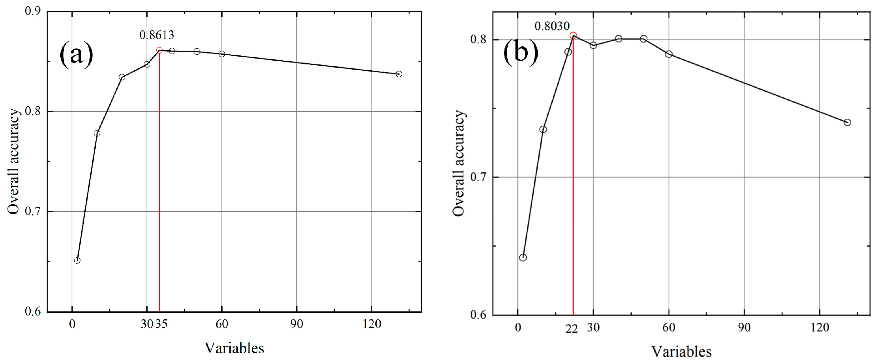
4.2.1. RFE-based Variable Selection Result

RFE-based variable selection for scenario 4 of GF-1 and ZY-3 data indicated that as the number of input variables increased, the overall accuracy of RF classifier first gradually rose until it reached 86.13% (ZY-3 is 80.30%), the highest overall accuracy, with a standard deviation of 3.43% (ZY-3 is 4.72%) at the 95% confidence interval when using 35 input variables (ZY-3 is 22). Then the overall accuracy decreased to 83.73% (ZY-3 is 73.98%), the lowest overall accuracy, with a standard deviation of 3.04% (ZY-3 is 4.02%) at the 95% confidence interval using all 131 input variables (Figure 5 and

Table 7. Overall accuracy of trained RF model using the RFE-based variable selection. OA: Overall accuracy; SD: Standard deviation.

Sensor	Order of Variables	OA (%)	SD(OA) (%)	Kappa (%)	SD(Kappa) (%)
GF-1	2	65.11	8.77	58.65	7.80
	10	77.81	4.40	73.70	5.25
	20	83.42	3.15	80.32	3.39
	30	84.70	3.22	81.86	3.41
	35	86.13	3.43	83.68	3.49
	40	86.03	3.83	83.41	3.76
	50	85.99	3.00	83.37	3.99
	60	85.74	3.38	83.08	3.41
	131	83.73	3.04	83.54	3.02
ZY-3	2	64.15	9.04	59.13	8.64
	10	73.47	5.14	68.39	5.79
	20	79.11	4.97	75.04	4.17
	22	80.30	4.72	76.44	4.06
	30	79.59	4.86	75.98	4.25
	40	80.07	4.45	76.88	4.33
	50	80.06	4.45	76.74	4.36
	60	78.95	4.41	74.83	4.25
	131	73.98	4.02	68.85	4.27

). Therefore, these 35 (ZY-3 is 22) input data were the most important variables and were selected as the final input variables after 10 cross-verifications. These 35 variables (ZY-3 is 22 variables) are mostly comprised of spectral bands, spectral indices, and textural information.

Spectral bands and spectral indices have the highest importance among all input variables. DEM, TWI, and slope were also essential input features for wetland vegetation mapping. In addition, the final input variables also included geometric data layers (compactness, area of segmented object, and shape index) and 19 textural data layers (Figure 6). After the RFE-based variable selection for scenario 4 of GF-1 data, the final input variables improved overall accuracy to 86.13%, an increase of 2.40% relative to using all 131 variables, and scenario 4 of ZY-3 data improved overall accuracy to 80.30%, an increase of 6.32% relative to using all 131 variables

4.2.2. Boruta-based Variable Selection Result

Boruta-based variable selection for scenario 4 of GF-1 and ZY-3 data found that as the number of input variables increased, the overall accuracy of RF classifier first kept increasing until it reached 85.07% (ZY-3 is 76.58%), the highest overall accuracy, with a standard deviation of 3.43% (ZY-3 is 4.31%) at the 95% confidence interval when using 76 input variables. However, the overall accuracy fell to 83.73% (ZY-3 is 73.98%), the lowest overall accuracy with a standard deviation of 3.32% (ZY-3 is 4.02%) at the 95% confidence interval when using all 131 variables (Figure 7 and

Table 8. Overall accuracy of trained RF model using Boruta-based variable selection. OA: overall accuracy; SD: standard deviation.

Sensor	Order of Variables	OA (%)	SD (OA) (%)	Kappa (%)	SD (Kappa) (%)
GF-1	2	65.11	6.48	59.38	7.79
	10	77.64	4.75	72.84	4.24
	20	83.50	3.16	80.50	3.70
	30	84.50	3.68	79.73	4.33
	40	84.51	3.92	80.88	4.65
	50	84.93	3.94	81.47	4.67
	60	84.58	4.07	81.58	4.79
	76	85.07	3.58	81.89	3.22
	80	84.84	3.17	80.78	3.76
	131	83.73	3.32	79.28	3.95
ZY-3	2	60.57	8.38	56.54	8.14
	10	68.69	7.25	64.47	7.22
	20	73.73	5.84	69.52	6.06
	30	75.40	4.68	71.44	5.23
	40	76.44	4.43	72.05	4.98
	50	76.30	4.35	72.11	4.57
	62	76.58	4.31	72.14	4.48
	70	76.45	4.22	73.25	4.39
	80	76.04	4.15	72.94	4.37
	131	73.98	4.02	68.85	4.27

). Therefore, 76 variables (ZY-3 is 62 variables) in scenario 4 of GF-1 data were confirmed and selected as the final input variables (Figure 8), and 53 variables (ZY-3 is 69 variables) were rejected after the RF model implemented training iterations 99 times.

The Boruta algorithm provided a z-score to measure the importance of input variables. In this paper, variables with an average z-score greater than 3.09 were confirmed and selected as important variables (Figure 8). Analysis of the final input variables found that NIR, red, and green bands, GNDVI and NDVI, textural mean, TWI, and slope layers all had higher z-scores than other variables, indicating that those input variables were more valuable for classifying marsh vegetation. This is consistent with the findings of RFE-based variable selection. Compared with the RFE algorithm, the Boruta algorithm selected more input variables, especially textural information, while the overall accuracy of the object-based RF classifier for scenario 4 using the variables derived from Boruta-based variable selection was lower than RFE-based variable selection. The results of GF-1 and ZY-3 data using Boruta-based variable selection indicated that the RFE algorithm had better performance than the Boruta algorithm in removing redundancy and reducing the dimensionality of multidimensional datasets.

4.2.3. VSURF-based Variable Selection Result

After 99 RF model iterations, VSURF-based variable selection for scenario 4 of GF-1 and ZY-3 data generated two subsets respectively. For scenario 4 of GF-1 data, the first subset retained 60 variables, including some redundant variables related to interpretation, and the second subset retained only 43 variables. For scenario 4 of ZY-3 data, the first subset retained 45 variables, including some redundant variables related to interpretation, and the second subset retained only 33 variables, which indicated that the second subset can better solve the problem of variable redundancy in marsh vegetation classification. As the number of input variables increased, the overall accuracy trend of the RF classifier for ZY-3 data is similar to that of GF-1 data (Figure 9). The overall accuracy of RF classifier for GF-1 data first increased to 85.73% (ZY-3 is 77.70%), the highest overall accuracy, with a standard deviation of 4.63% (ZY-3 is 4.68%) at the 95% confidence interval when using the second subset. Then the overall accuracy fell to 83.73% (ZY-3 is 73.98%), the lowest overall accuracy, with a standard deviation of 5.03% (ZY-3 is 4.02%) at the 95% confidence interval when all variables were used (Figure 9 and

Table 9. Overall accuracy of trained RF model using VSURF-based variable selection. OA: overall accuracy; SD: standard deviation.

Sensor	Order of Variables	OA (%)	SD (OA) (%)	Kappa (%)	SD (Kappa) (%)
GF-1	2	64.63	6.41	58.00	6.29
	10	78.54	4.57	73.90	5.37
	20	83.51	5.17	79.54	5.58
	30	85.03	4.93	82.47	4.07
	40	85.21	3.13	83.10	3.11
	43	85.60	3.63	83.31	3.54
	50	85.41	3.99	83.06	3.96
	60	84.80	3.51	82.37	3.58
	70	84.25	3.48	82.68	3.52
	131	83.73	3.03	81.49	3.01
ZY-3	2	61.54	7.75	53.96	8.37
	10	69.25	6.51	64.81	7.54
	20	74.32	5.48	69.87	6.34
	30	76.87	4.97	72.32	5.11
	33	77.70	4.68	73.25	4.69
	40	77.21	4.52	73.11	4.36
	45	76.89	4.28	72.84	4.23
	50	76.32	4.31	71.97	4.15
	60	76.11	4.08	71.54	4.18
	131	73.98	4.02	68.85	4.27

). It is worth mentioning that the overall accuracy was 84.83% (ZY-3 is 76.94%) for the first subset.

The input variables and their importance scores calculated by VSURF-based variable selection are shown in Figure 10. It can be seen that spectral bands and spectral indices were ranked at the top. DEM and TWI also performed well. In nine geometric data layers, only compactness, shape index, and max difference entered the second subset. The remaining variables were textural data layers. After the VSURF-based variable selection for scenario 4, the overall accuracy of classification was 85.60% (ZY-3 is 77.70%), and the overall accuracy of classification was improved 1.87% (ZY-3 is 3.72%); while performing data dimensionality reduction, the performance of VSURF was 0.53% (ZY-3 is 2.60%) lower than RFE-based variable selection, but 1.12% higher than Boruta-based variable selection.

The results derived from three variable selection algorithms in scenario 4 commonly demonstrated that blue red, green, and NIR bands, NDVI, GNDVI, RVI, and SWI were more important for RF-based wetland vegetation mapping, followed by DEM and TWI. There were more redundant variables in geometric and textural information (Figure A1). Among the three variable selection algorithms, the RFE-based algorithm performed best, followed by VSURF-based, and the performance of the Boruta-based algorithm in removing redundancy was inferior to the other two.

4.3. Visual Comparison and Accuracy Assessment of Classification Results

All classification scenarios of GF-1 and ZY-3 data provided an accurate visual depiction of land-cover types in the study area (Figure 11). According to the visualization results of GF-1 data and ZY-3 data, paddy field, shallow-water herbaceous vegetation, deep-water herbaceous vegetation, and shrub are easily to be confused because of poor spectral separability, which is particularly obvious in the ZY-3 data. GF-1 data can reduce pixel mixing to a certain extent due to its higher spatial resolution, which increases classification accuracy. By comparing the different classification scenarios of GF-1 and ZY-3 data, it is found that the classification result of scenario 4 (RFE) is more consistent with the actual vegetation distribution.

Accuracy assessment was performed for each classification scenario with the testing data. The overall classification accuracies for scenario 1, scenario 3, RFE-based, Boruta-based and VSURF-based scenario 4 of GF-1 and ZY-3 data are shown in

Table 10. Accuracy assessment of RF models for different classification scenarios using testing data.

Sensor	Scenario	Estimate (%)		Standard Error (%)	95% Confidence Intervals (%)
GF-1	1	Overall	81.87	3.97	77.59	85.63
		Kappa	78.36	3.60	74.90	82.78
	3	Overall	84.00	3.32	79.89	87.56
		Kappa	80.90	3.83	76.54	84.59
	4(RFE)	Overall	86.13	3.43	79.60	87.32
		Kappa	83.68	3.49	76.67	83.57
	4(Boruta)	Overall	85.07	3.58	79.60	87.32
		Kappa	81.89	3.22	76.67	83.57
	4(VSURF)	Overall	85.60	3.63	79.60	87.32
		Kappa	83.31	3.54	76.67	83.57
ZY-3	1	Overall	70.26	4.96	67.54	73.18
		Kappa	64.51	4.24	61.78	66.79
	3	Overall	74.42	4.65	71.62	77.14
		Kappa	69.77	4.37	66.80	72.55
	4(RFE)	Overall	80.30	4.72	77.43	83.25
		Kappa	76.44	4.06	74.37	78.89
	4(Boruta)	Overall	76.58	4.85	73.06	89.51
		Kappa	71.95	4.21	68.67	75.57
	4(VSURF)	Overall	77.70	4.77	74.24	80.53
		Kappa	73.24	4.16	70.12	76.57

. The classification results using GF-1 data were better than using ZY-3 data for all scenarios. The RFE-based RF algorithm using GF-1 data or ZY-3 data both achieved the highest overall classification accuracy. In the classification scenarios derived from GF-1 data, scenario 1 achieved the lowest overall accuracy (81.87%) with a standard error of 3.97% at the 95% confidence interval; Comparison of classification results derived from three variable selection algorithms, the RFE-based RF algorithms performed better than Boruta-based (85.07%)and VSURF-based (85.60%)algorithm. In the classification scenarios derived from ZY-3 data, scenario 1 achieved the lowest overall accuracy (70.26%) with a standard error of 4.96% at the 95% confidence interval; Comparison of classification results derived from three variable selection algorithms, the RFE-based RF algorithms performed better than Boruta-based (76.58%)and VSURF-based (77.70%) algorithm.

Detailed confusion matrix, user’s accuracy, and producer’s accuracy were summarized in

Table 11. Confusion matrix and associated classification accuracies based on testing data. A: forest; B: cropland; C: deep-water herbaceous vegetation; D: shallow-water herbaceous vegetation; E: shrub; F: open water; G: paddy field. T, total sample; P, producer accuracy (%); U, user accuracy (%); CI, 95% confidence interval (%).

		A	B	C	D	E	F	G	T	U	CI
Scenario 1 GF-1	A	82	0	0	0	3	0	0	85	96.5	93.2	98.8
	B	0	34	0	0	0	0	0	34	100.0	100.0	100.0
	C	0	0	30	3	4	3	1	41	73.2	69.9	76.8
	D	0	0	2	41	0	0	22	65	63.1	60.4	68.0
	E	1	8	3	2	69	0	0	83	83.1	80.6	86.3
	F	0	0	2	0	1	35	0	38	92.1	88.3	95.8
	G	0	0	0	13	0	0	16	29	55.1	53.0	58.8
	T	83	42	37	59	77	38	39
	P	98.8	81.0	81.1	69.5	89.6	92.1	41.0
	CI	95.1	77.8	77.9	66.4	84.8	87.7	38.5
		100.0	84.1	85.1	72.5	93.6	96.9	44.2
Scenario 3 GF-1	A	82	0	0	0	4	0	0	86	95.3	93.8	98.6
	B	0	37	0	3	1	1	0	42	88.1	85.8	92.6
	C	0	1	34	0	0	5	2	42	81.0	77.8	84.5
	D	0	0	1	45	1	1	22	70	64.3	60.7	67.4
	E	1	4	1	2	71	0	0	79	89.9	86.9	93.3
	F	0	0	1	0	0	31	0	32	96.9	93.2	98.9
	G	0	0	0	9	0	0	15	24	62.5	59.7	65.4
	T	83	42	37	59	77	38	39
	P	98.8	88.1	91.9	71.2	93.5	78.9	41.0
	CI	94.0	85.1	87.8	67.3	88.9	75.4	38.4
		100.0	93.2	94.9	74.6	97.4	81.8	44.6
Scenario 4 (RFE) GF-1	A	83	0	0	0	1	0	0	84	98.8	96.0	100.0
	B	0	36	1	1	0	0	0	38	94.7	91.6	97.1
	C	0	0	31	1	4	1	1	38	81.6	77.7	84.0
	D	0	2	0	51	3	0	22	78	65.4	62.7	68.4
	E	0	4	0	1	69	0	0	74	93.2	90.1	96.7
	F	0	0	5	0	0	37	0	42	88.1	84.6	91.2
	G	0	0	0	5	0	0	16	21	76.2	73.2	80.0
	T	83	42	37	59	77	38	39
	P	100.0	88.1	83.8	86.4	89.6	97.4	41.0
	CI	100.0	88.4	80.4	83.3	86.9	94.7	38.1
		100.0	97.1	87.0	89.1	92.6	99.9	44.4
Scenario 1 ZY-3	A	55	0	0	0	11	1	0	67	82.1	78.5	85.3
	B	0	19	0	2	4	0	0	25	76.0	72.6	79.5
	C	0	0	20	6	2	5	2	35	57.1	54.3	60.4
	D	0	0	3	22	1	0	8	34	64.7	61.7	67.9
	E	3	5	2	2	38	6	1	57	66.7	62.8	70.1
	F	0	0	3	0	1	15	0	19	78.9	75.3	82.2
	G	0	1	0	10	1	0	20	32	62.5	59.3	65.8
	T	58	25	28	42	58	27	31
	P	94.8	76.0	71.4	52.4	65.5	55.6	64.5
	CI	91.5	72.6	68.1	48.6	62.4	52.3	61.7
		97.4	79.7	74.9	56.3	68.9	58.4	67.8
Scenario 3ZY-3	A	56	0	0	0	3	1	0	60	93.3	91.0	96.2
	B	0	19	0	0	1	0	0	20	95.0	91.8	98.3
	C	0	0	22	4	2	5	0	33	66.7	63.5	70.0
	D	0	0	0	24	2	0	20	46	52.2	49.1	55.4
	E	2	6	2	1	50	1	1	63	79.4	76.3	82.8
	F	0	0	4	0	0	20	0	24	83.3	80.5	86.4
	G	0	0	0	13	0	0	10	23	43.5	40.2	47.1
	T	58	25	28	42	58	27	31
	P	96.6	76.0	78.6	57.1	86.2	74.1	32.3
	CI	93.2	72.3	75.6	54.0	82.9	71.5	29.1
		99.4	78.9	81.2	60.8	89.6	77.7	35.4
Scenario 4 (RFE) ZY-3	A	58	1	0	0	4	1	0	64	90.6	87.4	93.7
	B	0	19	0	2	0	0	0	21	90.5	87.5	93.2
	C	0	0	20	3	1	5	1	30	66.7	63.2	70.3
	D	0	2	0	30	1	0	12	45	66.7	62.4	70.6
	E	0	3	1	2	52	1	1	60	86.7	83.3	90.0
	F	0	0	6	1	0	20	0	27	74.1	71.5	77.7
	G	0	0	1	4	0	0	17	22	77.3	74.1	80.4
	T	58	25	28	42	58	27	31
	P	100.0	76.0	71.4	71.4	89.7	74.1	54.8
	CI	100.0	73.1	68.1	68.5	86.8	70.9	51.5
		100.0	79.4	74.3	71.6	92.4	77.0	57.9

. In the four classification scenarios without variable selection based on GF-1 data, forest achieved the highest user’s accuracy (higher than 94.3%). Open water, cropland, and shrub all achieved over 83.1% user’s accuracy. Paddy field had the lowest user’s accuracy (below 62.5%) for all vegetation classes. Variable selection for scenario 4 of GF-1 data improved the classification accuracy of paddy field and achieved over 66.7% user’s accuracy. Comparison of three variable selection algorithms, scenario 4 based on RFE algorithm achieved the highest user’s accuracy (76.2%) for paddy field. Shallow-water herbaceous vegetation produced the lowest user’s accuracy because of easily confusion with paddy field. In addition, in all classification scenarios without variable selection based on ZY-3 data, forest and open water achieved highest classification accuracy for all vegetation classes, with more than 78.9% user’s accuracy. Cropland and shrub produced over 66.7% user’s accuracy. Paddy field achieved below 62.5% user’s accuracy, which are similar to the classification accuracy using GF-1 data. It is worth mentioning that scenario 4 of ZY-3 data based on the RFE algorithm for variable selection obviously improved classification accuracy of shallow-water herbaceous vegetation and paddy field. However, the classification accuracy of each vegetation class except for shallow-water herbaceous vegetation and paddy field using ZY-3 data is lower than that of using GF-1 data due to the coarse spatial resolution of ZY-3 data.

McNemar’s chi-square test (

Table 12. McNemar’s statistic comparing the classification of each scenario.

Sensor	Comparisons	Scenario 1	Scenario 3	Scenario 4 (RFE)	Scenario 4 (Boruta)	Scenario 4 (VSURF)
GF-1	Scenario 1	–	2.00	2.67	1.42	3.15
	Scenario 3		–	2.91	1.14	1.80
	Scenario 4 (RFE)			–	2.23	0.25
	Scenario 4 (Boruta)				–	0.06
	Scenario 4 (VSURF)					–
ZY-3	Scenario 1	–	3.52	8.25	4.58	5.27
	Scenario 3		–	5.53	3.41	4.19
	Scenario 4 (RFE)			–	3.32	1.87
	Scenario 4 (Boruta)				–	1.69
	Scenario 4 (VSURF)					–

Differences are significant at the 95% confidence level (McNemar’s test |z| > 1.96) [62].

) revealed that there are significant differences between classification scenarios 1, 3, and 4 of GF-1 and ZY-3 data at the 95% confidence level. When comparing classification results derived from GF-1 data, there were statistically significant differences between scenario 1 and other three classification scenarios with the except of scenario 4 (Boruta). There are also significant differences between scenario 3 and scenario 4 (RFE). When comparing classification results derived from ZY-3 data, there were statistically significant differences between scenario 1 and the other four classification scenarios. Meanwhile, there were statistically significant differences between scenario 3 and scenario 4 based on three variable selection algorithms. For scenario 4 of GF-1 and ZY-3 data, the difference between RFE-based and Boruta-based classifications is statistically significant.

5. Discussion

Previous studies reported that the default number of mtry in the RF algorithm is the square of the total number of input variables, and the default number of ntrees is 500 [74,75]. In this study, if the default parameters (mtry, ntrees) were used, the parameter settings for the four classification scenarios of GF-1 data were (5, 500), (5, 500), (6, 500), and (11, 500). However, after parameter optimization of the RF algorithm, the optimal parameters after 15 iterations for the four classification scenarios of GF-1 data were (6, 1450), (6, 1550), (5, 1400), and (10, 1450). Although the RF algorithm used the default parameters for HNNR marsh vegetation identification with high overall accuracy, it is extremely unstable and unrepresentative. Compared with the default parameters, the overall accuracy of optimal parameters was more stable, which meets the needs of this study. The results of parameter optimization for the four classification scenarios of ZY-3 data also support this conclusion, which indicated that the default parameters of the RF algorithm are not applicable to HNNR marsh vegetation classification because of its poor stability [76,77].

In addition, previous studies reported that fusing multidimensional datasets for classification of land-use types could improve classification accuracy [78]. In this study, scenario 1 (24 input variables), scenario 2 (26 input variables), and scenario 3 (35 input variables) of GF-1 and ZY-3 data with increased input variables had higher classification accuracy, but the classification accuracy for scenario 4 (131 input variables) of GF-1 data decreased by 0.27% (ZY-3 is 0.74%) compared to scenario 3 (35 input variables). This result indicated that the texture information contains a lot of redundant variables, which reduces the calculation efficiency and overall accuracy of classification. Therefore, it is important to reduce the dimensionality of large multidimensional datasets, eliminate redundant variables and retain effective variables [79,80]. This study performed three RF-based variable selection algorithms for scenario 4 of GF-1 and ZY-3 data to obtain optimum and stable classification [81,82]. Compared with scenario 4 with an initial 131 input layers, the RFE algorithm for GF-1 data only selected 35 (ZY-3 is 22) variables to develop the classification model, and achieved the highest overall accuracy is 86.13% (ZY-3 is 80.30%) with 3.43% (ZY-3 is 4.02%) standard error at the 95% confidence interval. The VSURF algorithm for GF-1 data selected 43 (ZY-3 is 33) variables to develop the classification model and achieved 85.60% (ZY-3 is 77.70%) overall accuracy with 3.63% (ZY-3 is 4.68%) standard error at the 95% confidence interval. The Boruta algorithm for GF-1 data had the worst effect in eliminating redundant variables; 76 (ZY-3 is 62) variables were selected to develop the classification model, and overall accuracy was 86.13% (ZY-3 is 76.58%) with 3.58% (ZY-3 is 4.31%) standard error at the 95% confidence interval. Among the three variable selection algorithms for GF-1 and ZY-3 data, the RFE algorithm had the best dimensionality reduction performance, followed by the VSURF algorithm, and the Boruta algorithm had the worst performance. The results show that dimensionality reduction of high-dimensional variables can improve the classification accuracy while improving the efficiency of the classifier [83].

The three variable selection algorithms based on RF algorithm could rank the importance of input variables of scenario 4, which is important to further exploration of the different variables on the accuracy of swamp wetland vegetation identification [84]. The RFE, Boruta, and VSURF algorithms for GF-1 and ZY-3 data found that four optical spectral bands, four spectral indices, GLCM_Mean_2 (mean value of green band in textural information), GLCM_Mean_4 (mean value of NIR band in textural information), DEM and TWI were more useful for discriminating marsh vegetation in HNNR. DEM and TWI are highly correlated with soil moisture content and surface water pooling and has been demonstrated to provide good measurement of wetland location and boundaries [85]. DEM and TWI as important input variables in the classification model, improved the ability to discriminate shallow-water and deep-water herbaceous vegetation. In addition, compactness, max difference, and shape index in geometric information also contribute to the preparation of swamps. These conclusions demonstrate that when using the RF model for marsh vegetation classification with remote sensing data, parameter optimization and variable selection should be conducted to improve classification diagnostics and performance.

Applying high-resolution remote sensing images can improve the accuracy of vegetation mapping to a certain extent [41,86]. The object-based classifications produced by GF-1 images consistently achieved more than 81% overall accuracy, indicating that GF-1 images are a valuable data source to discriminate marsh vegetation. The overall accuracy of object-based classifications produced by ZY-3 images is between 70.26% and 80.30%, which indicated that limited by the spatial resolution of ZY-3 data (5.8 m), and its performance of application to marsh vegetation mapping with intricate vegetation distribution is inferior to GF-1 data (2 m) with higher spatial resolution. GF-1 and ZY-3 data in this study had higher classification accuracy for forest, cropland, shrubs, and open water than other vegetation types because of the spectral differences; the spectral difference between forest and shrubs is small, but the textural and geometric information are different, and the spectral indices can distinguish the two to a certain extent. However, limited by the spectral resolution and spectral range (450–900 nm), GF-1 and ZY-3 data in this study had low classification accuracy for deep-water herbaceous vegetation, shallow-water herbaceous vegetation, and paddy field because of the subtle differences of the spectral response and similar textural. Future studies will use high spatial resolution hyperspectral satellite images or low-altitude UAV images of different growing seasons in high-precision marsh vegetation mapping.

6. Conclusions

The object-based RF algorithm was used to evaluate the performance of GF-1 and ZY-3 data on marsh vegetation mapping. This study attempted to customize an object-based RF model suitable for marsh vegetation through multiscale image segmentation, parameter optimization, multidimensional dataset input, and variable selection and explored the differences in accuracy of different parameter settings and variable inputs. Some important conclusions are that parameter optimization of the RF model can effectively improve its applicability in marsh vegetation classification, obtaining stable high accuracy. Combining spectral bands, spectral indices, textural information, and geometric information as multidimensional dataset input variables can effectively improve the classification accuracy of marsh vegetation. However, multidimensional dataset input generates many redundant variables, which reduces classification efficiency and accuracy. The RF-based variable selection algorithms can effectively remove redundant variables with high correlation and improve classification accuracy. Compared with Boruta-based and VSURF-based variable selection, RFE-based is a more efficient variable selection algorithm. Measurements of the importance of the input variables indicated that four optical spectral bands, four spectral indices, mean value of green and NIR bands in textural information, DEM, TWI, compactness, max difference, and shape index were more useful for distinguishing marsh vegetation in HNNR. The classification results show that GF-1 and ZY-3 images are valuable source of data for distinguishing marsh vegetation, and the performance of ZY-3 images that application to marsh vegetation mapping is inferior to GF-1 images in HNNR. GF-1 and ZY-3 images had higher classification accuracy for forest, cropland, shrubs, and open water. However, limited by spectral resolution and spectral range, GF-1 had low classification accuracy for deep-water herbaceous vegetation, shallow-water herbaceous vegetation, and paddy fields.

References

1. Henderson, F.M.; Lewis, A.J. Radar detection of wetland ecosystems: A review. Int. J. Remote Sens. 2008, 29, 5809–5835. [Google Scholar] [CrossRef]
2. Betbeder, J.; Rapinel, S.; Corpetti, T.; Pottier, E.; Corgne, S.; Hubert-Moy, L. Multitemporal classification of TerraSAR-X data for wetland vegetation mapping. J. Appl. Remote Sens. 2014, 8, 083648. [Google Scholar] [CrossRef]
3. Zhou, D.; Gong, H.; Wang, Y.; Khan, S.; Zhao, K. Driving forces for the marsh wetland degradation in the Honghe National Nature Reserve in Sanjiang Plain, Northeast China. Environ. Model. Assess. 2009, 14, 101–111. [Google Scholar] [CrossRef]
4. Adam, E.; Mutanga, O.; Rugege, D. Multispectral and hyperspectral remote sensing for identification and mapping of marsh wetland vegetation: A review. Wetl. Ecol. Manag. 2010, 18, 281–296. [Google Scholar] [CrossRef]
5. Millard, K.; Richardson, M. Wetland mapping with LiDAR derivatives, SAR polarimetric decompositions, and LiDAR–SAR fusion using a random forest classifier. Can. J. Remote Sens. 2013, 39, 290–307. [Google Scholar] [CrossRef]
6. Zedler, J.B.; Kercher, S. Wetland resources: Status, trends, ecosystem services, and restorability. Annu. Rev. Environ. Resour. 2005, 30, 39–74. [Google Scholar] [CrossRef] [Green Version]
7. Kokaly, R.F.; Despain, D.G.; Clark, R.N.; Livo, K.E. Mapping vegetation in Yellowstone National Park using spectral feature analysis of AVIRIS data. Remote Sens. Environ. 2003, 84, 437–456. [Google Scholar] [CrossRef] [Green Version]
8. Ramsey, E.; Rangoonwala, A.; Middleton, B.; Lu, Z. Satellite optical and radar data used to track wetland forest impact and short-term recovery from Hurricane Katrina. Wetlands 2009, 29, 66–79. [Google Scholar] [CrossRef] [Green Version]
9. Jenkins, R.B.; Frazier, P.S. High-resolution remote sensing of upland swamp boundaries and vegetation for baseline mapping and monitoring. Wetlands 2010, 30, 531–540. [Google Scholar] [CrossRef]
10. Frohn, R.C.; Autrey, B.C.; Lane, C.R.; Reif, M. Segmentation and object-oriented classification of wetlands in a karst Florida landscape using multi-season Landsat-7 ETM+ imagery. Int. J. Remote Sens. 2011, 32, 1471–1489. [Google Scholar] [CrossRef]
11. Tuxen, K.; Schile, L.; Stralberg, D.; Siegel, S.; Parker, T.; Vasey, M.; Callaway, J.; Kelly, M. Mapping changes in tidal wetland vegetation composition and pattern across a salinity gradient using high spatial resolution imagery. Wetl. Ecol. Manag. 2011, 19, 141–157. [Google Scholar] [CrossRef]
12. Zhang, Y.; Lu, D.; Yang, B.; Sun, C.; Sun, M. Coastal wetland vegetation classification with a Landsat Thematic Mapper image. Int. J. Remote Sens. 2011, 32, 545–561. [Google Scholar] [CrossRef]
13. Abeysinghe, T.; Simic Milas, A.; Arend, K.; Hohman, B.; Reil, P.; Gregory, A.; Vázquez-Ortega, A. Mapping invasive phragmites australis in the Old Woman Creek Estuary using UAV remote sensing and machine learning classifiers. Remote Sens. 2019, 11, 1380. [Google Scholar] [CrossRef] [Green Version]
14. Wietecha, M.; Jełowicki, Ł.; Mitelsztedt, K.; Miścicki, S.; Stereńczak, K. The capability of species-related forest stand characteristics determination with the use of hyperspectral data. Remote Sens. Environ. 2019, 231, 111232. [Google Scholar] [CrossRef]
15. Sang, X.; Guo, Q.; Wu, X.; Fu, Y.; Xie, T.; He, C.; Zang, J. Intensity and stationarity analysis of land use change based on CART algorithm. Sci. Rep. 2019, 9, 1–12. [Google Scholar] [CrossRef] [Green Version]
16. Li, W.; El-Askary, H.; Qurban, M.A.; Li, J.; ManiKandan, K.P.; Piechota, T. Using multi-indices approach to quantify mangrove changes over the Western Arabian Gulf along Saudi Arabia coast. Ecol. Indic. 2019, 102, 734–745. [Google Scholar] [CrossRef]
17. Mahdianpari, M.; Salehi, B.; Mohammadimanesh, F.; Homayouni, S.; Gill, E. The first wetland inventory map of newfoundland at a spatial resolution of 10 m using sentinel-1 and sentinel-2 data on the google earth engine cloud computing platform. Remote Sens. 2019, 11, 43. [Google Scholar] [CrossRef] [Green Version]
18. Amani, M.; Salehi, B.; Mahdavi, S.; Brisco, B. Spectral analysis of wetlands using multi-source optical satellite imagery. ISPRS J. Photogramm. 2018, 144, 119–136. [Google Scholar] [CrossRef]
19. Fu, B.; Wang, Y.; Campbell, A.; Li, Y.; Zhang, B.; Yin, S.; Jin, X. Comparison of object-based and pixel-based Random Forest algorithm for marsh wetland vegetation mapping using high spatial resolution GF-1 and SAR data. Ecol. Indic. 2017, 73, 105–117. [Google Scholar] [CrossRef]
20. Dronova, I.; Gong, P.; Wang, L. Object-based analysis and change detection of major wetland cover types and their classification uncertainty during the low water period at Poyang Lake, China. Remote Sens. Environ. 2011, 115, 3220–3236. [Google Scholar] [CrossRef]
21. Boyden, J.; Joyce, K.E.; Boggs, G.; Wurm, P. Object-based mapping of native vegetation and para grass (Urochloa mutica) on a monsoonal wetland of Kakadu NP using a Landsat 5 TM Dry-season time series. J. Spat. Sci. 2013, 58, 53–77. [Google Scholar] [CrossRef]
22. Dronova, I. Object-based image analysis in wetland research: A review. Remote Sens. 2015, 7, 6380–6413. [Google Scholar] [CrossRef] [Green Version]
23. Dronova, I.; Gong, P.; Wang, L.; Zhong, L. Mapping dynamic cover types in a large seasonally flooded wetland using extended principal component analysis and object-based classification. Remote Sens. Environ. 2015, 158, 193–206. [Google Scholar] [CrossRef]
24. Mui, A.; He, Y.; Weng, Q. An object-based approach to delineate wetlands across landscapes of varied disturbance with high spatial resolution satellite imagery. ISPRS J. Photogramm. 2015, 109, 30–46. [Google Scholar] [CrossRef] [Green Version]
25. Dronova, I.; Gong, P.; Clinton, N.E.; Wang, L.; Fu, W.; Qi, S.; Liu, Y. Landscape analysis of wetland plant functional types: The effects of image segmentation scale, vegetation classes and classification methods. Remote Sen. Environ. 2012, 127, 357–369. [Google Scholar] [CrossRef]
26. Chen, Y.; Niu, Z.; Johnston, C.A.; Hu, S. A Unifying Approach to Classifying Wetlands in the Ontonagon River Basin, Michigan, Using Multi-temporal Landsat-8 OLI Imagery. Can. J. Remote Sens. 2018, 44, 373–389. [Google Scholar] [CrossRef]
27. Ludwig, C.; Walli, A.; Schleicher, C.; Weichselbaum, J.; Riffler, M. A highly automated algorithm for wetland detection using multi-temporal optical satellite data. Remote Sens. Environ. 2019, 224, 333–351. [Google Scholar] [CrossRef]
28. Mahdianpari, M.; Salehi, B.; Mohammadimanesh, F.; Motagh, M. Random forest wetland classification using ALOS-2 L-band, RADARSAT-2 C-band, and TerraSAR-X imagery. ISPRS J. Photogramm. 2017, 130, 13–31. [Google Scholar] [CrossRef]
29. Merchant, M.A.; Warren, R.K.; Edwards, R.; Kenyon, J.K. An object-based assessment of multi-wavelength SAR, optical imagery and topographical datasets for operational wetland mapping in Boreal Yukon, Canada. Can. J. Remote Sens. 2019, 45, 308–332. [Google Scholar] [CrossRef]
30. Mohammadimanesh, F.; Salehi, B.; Mahdianpari, M.; Motagh, M.; Brisco, B. An efficient feature optimization for wetland mapping by synergistic use of SAR intensity, interferometry, and polarimetry data. Int. J. Appl. Earth Obs. 2018, 73, 450–462. [Google Scholar] [CrossRef]
31. Ghosh, A.; Joshi, P.K. A comparison of selected classification algorithms for mapping bamboo patches in lower Gangetic plains using very high resolution WorldView 2 imagery. Int. J. Appl. Earth Obs. 2014, 26, 298–311. [Google Scholar] [CrossRef]
32. Räsänen, A.; Kuitunen, M.; Tomppo, E.; Lensu, A. Coupling high-resolution satellite imagery with ALS-based canopy height model and digital elevation model in object-based boreal forest habitat type classification. ISPRS J. Photogramm. 2014, 94, 169–182. [Google Scholar] [CrossRef] [Green Version]
33. Speiser, J.L.; Miller, M.E.; Tooze, J.; Ip, E. A comparison of Random Forest variable selection methods for classification prediction modeling. Expert Syst. Appl. 2019, 134, 93–101. [Google Scholar] [CrossRef]
34. Chunling, L.; Zhaoguang, B. Characteristics and typical applications of GF-1 satellite. In Proceedings of the 2015 IEEE International Geoscience and Remote Sensing Symposium, Milan, Italy, 26–31 July 2015; pp. 1246–1249. [Google Scholar]
35. Cao, H.; Gao, W.; Zhang, X.; Liu, X.; Fan, B.; Li, S. Overview of ZY-3 satellite research and application. In Proceedings of the 63rd IAC (International Astronautical Congress), Naples, Italy, 1–5 October 2012. [Google Scholar]
36. Johnston, K.; Ver Hoef, J.M.; Krivoruchko, K.; Lucas, N. Using ArcGIS Geostatistical Analyst; Esri: Redlands, CA, USA, 2001. [Google Scholar]
37. Exelis, V.I.S. ENVI 5.3; Exelis VIS: Boulder, CO, USA, 2015. [Google Scholar]
38. Kaufman, Y.J.; Wald, A.E.; Remer, L.A.; Gao, B.; Li, R.; Flynn, L. The modis 2.1-μm channel-correlation with visible reflectance for use in remote sensing of aerosol. IEEE Trans. Geosci. Remote 1997, 35, 1286–1298. [Google Scholar] [CrossRef]
39. Laben, C.A.; Brower, B.V. Process for enhancing the spatial resolution of multispectral imagery using pan-sharpening. U.S. Patent 6,011,875, 4 January 2000. [Google Scholar]
40. Cho, M.A.; Malahlela, O.; Ramoelo, A. Assessing the utility WorldView-2 imagery for tree species mapping in South African subtropical humid forest and the conservation implications: Dukuduku forest patch as case study. Int. J. Appl. Earth Obs. 2015, 38, 349–357. [Google Scholar] [CrossRef]
41. Xu, K.; Tian, Q.; Yang, Y.; Yue, J.; Tang, S. How up-scaling of remote-sensing images affects land-cover classification by comparison with multiscale satellite images. Int. J. Remote Sens. 2019, 40, 2784–2810. [Google Scholar] [CrossRef]
42. Rampi, L.P.; Knight, J.F.; Pelletier, K.C. Wetland mapping in the upper midwest United States. Photogramm. Eng. Rem. Sens. 2014, 80, 439–448. [Google Scholar] [CrossRef]
43. Maxwell, A.E.; Warner, T.A.; Strager, M.P. Predicting palustrine wetland probability using random forest machine learning and digital elevation data-derived terrain variables. Photogramm. Eng. Rem. Sens. 2016, 82, 437–447. [Google Scholar] [CrossRef]
44. Shawky, M.; Moussa, A.; Hassan, Q.K.; El-Sheimy, N. Pixel-based geometric assessment of channel networks/orders derived from global spaceborne digital elevation models. Remote Sens. 2019, 11, 235. [Google Scholar] [CrossRef] [Green Version]
45. Haralick, R.M.; Shanmugam, K.; Dinstein, I.H. Textural features for image classification. IEEE Trans. Syst. Man Cybern. 1973, 6, 610–621. [Google Scholar] [CrossRef] [Green Version]
46. Szantoi, Z.; Escobedo, F.; Abd-Elrahman, A.; Smith, S.; Pearlstine, L. Analyzing fine-scale wetland composition using high resolution imagery and texture features. Int. J. Appl. Earth Obs. 2013, 23, 204–212. [Google Scholar] [CrossRef]
47. Hidayat, S.; Matsuoka, M.; Baja, S.; Rampisela, D. Object-based image analysis for sago palm classification: The most important features from high-resolution satellite imagery. Remote Sens. 2018, 10, 1319. [Google Scholar] [CrossRef] [Green Version]
48. Tian, S.; Zhang, X.; Tian, J.; Sun, Q. Random forest classification of wetland landcovers from multi-sensor data in the arid region of Xinjiang, China. Remote Sens. 2016, 8, 954. [Google Scholar] [CrossRef] [Green Version]
49. Lu, D.; Li, G.; Moran, E.; Dutra, L.; Batistella, M. The roles of textural images in improving land-cover classification in the Brazilian Amazon. Int. J. Remote Sens. 2014, 35, 8188–8207. [Google Scholar] [CrossRef] [Green Version]
50. Szantoi, Z.; Escobedo, F.; Abd-Elrahman, A.; Pearlstine, L.; Dewitt, B.; Smith, S. Classifying spatially heterogeneous wetland communities using machine learning algorithms and spectral and textural features. Environ. Monit. Assess. 2015, 187, 262. [Google Scholar] [CrossRef]
51. eCognition Developer, T. 9.0 User Guide; Trimble Germany GmbH: Munich, Germany, 2014. [Google Scholar]
52. Rouse, J.W.; Haas, R.H.; Schell, J.A.; Deering, D.W. Monitoring Vegetation Systems in the Great Plains with ERTS. In Third Earth Resources Technology Satellite-1 Symposium; NASA: Washington, DC, USA, 1973; pp. 309–317. [Google Scholar]
53. Major, D.J.; Baret, F.; Guyot, G. A ratio vegetation index adjusted for soil brightness. Int. J. Remote Sens. 1990, 11, 727–740. [Google Scholar] [CrossRef]
54. Gitelson, A.; Spivak, L.; Zakarin, E.; Kogan, F.; Lebed, L. Estimation of seasonal dynamics of pasture and crop productivity in Kazakhstan using NOAA/AVHRR data. In Proceedings of the IGARSS’96. 1996 International Geoscience and Remote Sensing Symposium, Lincoln, NE, USA, 31–31 May 1996. [Google Scholar]
55. Mallick, K.; Bhattacharya, B.K.; Patel, N.K. Estimating volumetric surface moisture content for cropped soils using a soil wetness index based on surface temperature and NDVI. Agr. Forest Meteorol. 2009, 149, 1327–1342. [Google Scholar] [CrossRef]
56. Sörensen, R.; Zinko, U.; Seibert, J. On the calculation of the topographic wetness index: Evaluation of different methods based on field observations. Hydrol. Earth Syst. Sci. 2006, 10, 101–112. [Google Scholar] [CrossRef] [Green Version]
57. Inglada, J. Automatic recognition of man-made objects in high resolution optical remote sensing images by SVM classification of geometric image features. ISPRS J. Photogramm. 2007, 62, 236–248. [Google Scholar] [CrossRef]
58. Moffett, K.B.; Gorelick, S.M. Distinguishing wetland vegetation and channel features with object-based image segmentation. Int. J. Remote Sens. 2013, 34, 1332–1354. [Google Scholar] [CrossRef]
59. Drǎguţ, L.; Tiede, D.; Levick, S.R. ESP: A tool to estimate scale parameter for multiresolution image segmentation of remotely sensed data. Int. J. Geogr. Inf. Sci. 2010, 24, 859–871. [Google Scholar] [CrossRef]
60. Breiman, L. Random forests. Mach. Learn. 2001, 45, 5–32. [Google Scholar] [CrossRef] [Green Version]
61. Phiri, D.; Morgenroth, J.; Xu, C. Four decades of land cover and forest connectivity study in Zambia—An object-based image analysis approach. Int. J. Appl. Earth. Obs. 2019, 79, 97–109. [Google Scholar] [CrossRef]
62. Genuer, R.; Poggi, J.M.; Tuleau-Malot, C. Variable selection using random forests. Pattern Recogn. Lett. 2010, 31, 2225–2236. [Google Scholar] [CrossRef] [Green Version]
63. Silveira, E.M.; Silva, S.H.G.; Acerbi-Junior, F.W.; Carvalho, M.C.; Carvalho, L.M.T.; Scolforo, J.R.S.; Wulder, M.A. Object-based random forest modelling of aboveground forest biomass outperforms a pixel-based approach in a heterogeneous and mountain tropical environment. Int. J. Appl. Earth Obs. 2019, 78, 175–188. [Google Scholar] [CrossRef]
64. Liaw, A.; Wiener, M. The randomforest package. R News 2002, 2, 18–22. [Google Scholar]
65. Team, R.C. R: A language and environment for statistical computing. Available online: http://http://cran.fhcrc.org/web/packages/dplR/vignettes/intro-dplR.pdf (accessed on 15 April 2020).
66. Kuhn, M. Variable Selection Using the Caret Package. Available online: http://cran.r-project.org/web/packages/caret/vignettes/caretSelection.pdf (accessed on 15 April 2020).
67. Kursa, M.B.; Rudnicki, W.R. Feature selection with the Boruta package. J. Stat. Softw. 2010, 36, 1–13. [Google Scholar] [CrossRef] [Green Version]
68. Genuer, R.; Poggi, J.M.; Tuleaumalot, C. VSURF: An R package for variable selection using Random Forests. R. J. 2015, 7, 19–33. [Google Scholar] [CrossRef] [Green Version]
69. Olofsson, P.; Foody, G.M.; Herold, M.; Stehman, S.V.; Woodcock, C.E.; Wulder, M.A. Good practices for estimating area and assessing accuracy of land change. Remote Sens. Environ. 2014, 148, 42–57. [Google Scholar] [CrossRef]
70. Phiri, D.; Morgenroth, J.; Xu, C.; Hermosilla, T. Effects of pre-processing methods on Landsat OLI-8 land cover classification using OBIA and random forests classifier. Int. J. Appl. Earth. Obs. 2018, 73, 170–178. [Google Scholar] [CrossRef]
71. Foody, G.M. Thematic map comparison: Evaluating the Statistical significance of differences in classification accuracy. Photogramm. Eng. Rem. Sens. 2004, 70, 627–634. [Google Scholar] [CrossRef]
72. Duro, D.C.; Franklin, S.E.; Dubé, M.G. A comparison of pixel-based and object-based image analysis with selected machine learning algorithms for the classification of agricultural landscapes using SPOT-5 HRG imagery. Remote Sens. Environ. 2012, 118, 259–272. [Google Scholar] [CrossRef]
73. Thanh Noi, P.; Kappas, M. Comparison of random forest, k-nearest neighbor, and support vector machine classifiers for land cover classification using Sentinel-2 imagery. Sensors 2018, 18, 18. [Google Scholar] [CrossRef] [PubMed] [Green Version]
74. Stumpf, A.; Kerle, N. Object-oriented mapping of landslides using Random Forests. Remote Sens. Environ. 2011, 115, 2564–2577. [Google Scholar] [CrossRef]
75. Nguyen, U.; Glenn, E.P.; Dang, T.D.; Pham, L.T. Mapping vegetation types in semi-arid riparian regions using random forest and object-based image approach: A case study of the Colorado River Ecosystem, Grand Canyon, Arizona. Ecol. Inform. 2019, 50, 43–50. [Google Scholar] [CrossRef]
76. Zhang, Y.; Zhang, H.; Lin, H. Improving the impervious surface estimation with combined use of optical and SAR remote sensing images. Remote Sens. Environ. 2014, 141, 155–167. [Google Scholar] [CrossRef]
77. Ming, D.; Zhou, T.; Wang, M.; Tan, T. Land cover classification using random forest with genetic algorithm-based parameter optimization. J. Appl. Remote Sens. 2016, 10, 035021. [Google Scholar] [CrossRef]
78. Zhang, H.; Li, Q.; Liu, J.; Shang, J.; Du, X.; McNairn, H.; Champagne, C.; Dong, T.; Liu, M. Image classification using rapideye data: Integration of spectral and textual features in a random forest classifier. IEEE J. STARS. 2017, 10, 5334–5349. [Google Scholar] [CrossRef]
79. Georganos, S.; Grippa, T.; Vanhuysse, S.; Lennert, M.; Shimoni, M.; Kalogirou, S.; Wolff, E. Less is more: Optimizing classification performance through feature selection in a very-high-resolution remote sensing object-based urban application. GISci. Remote Sens. 2018, 55, 221–242. [Google Scholar] [CrossRef]
80. Lagrange, A.; Fauvel, M.; Grizonnet, M. Large-scale feature selection with Gaussian mixture models for the classification of high dimensional remote sensing images. IEEE Trans. Comput. Imaging 2017, 3, 230–242. [Google Scholar] [CrossRef] [Green Version]
81. Millard, K.; Richardson, M. On the importance of training data sample selection in random forest image classification: A case study in peatland ecosystem mapping. Remote Sens. 2015, 7, 8489–8515. [Google Scholar] [CrossRef] [Green Version]
82. Shih, H.C.; Stow, D.A.; Tsai, Y.H. Guidance on and comparison of machine learning classifiers for Landsat-based land cover and land use mapping. Int. J. Remote Sens. 2019, 40, 1248–1274. [Google Scholar] [CrossRef]
83. Lim, J.; Kim, K.M.; Jin, R. Tree species classification using Hyperion and Sentinel-2 Data with machine learning in South Korea and China. ISPRS. Int. J. Geo-Inf. 2019, 8, 150. [Google Scholar] [CrossRef] [Green Version]
84. Gumbricht, T. Detecting trends in wetland extent from MODIS derived soil moisture estimates. Remote Sens. 2018, 10, 611. [Google Scholar] [CrossRef] [Green Version]
85. Berhane, T.; Lane, C.; Wu, Q.; Autrey, B.; Anenkhonov, O.; Chepinoga, V.; Liu, H. Decision-tree, rule-based, and random forest classification of high-resolution multispectral imagery for wetland mapping and inventory. Remote Sens. 2018, 10, 580. [Google Scholar] [CrossRef] [Green Version]
86. McCarthy, M.J.; Radabaugh, K.R.; Moyer, R.P.; Muller-Karger, F.E. Enabling efficient, large-scale high-spatial resolution wetland mapping using satellites. Remote Sens. Environ. 2018, 208, 189–201. [Google Scholar] [CrossRef]
Figure 1. Study area (Gaofen-1 (GF-1) false-color image display: bands 4, 3, 2 in red, green, blue (RGB)) and vegetation associations. (a) Salix brachypoda; (b) shallow-water plants; (c) Betula platyphylla forest.
Remotesensing 12 01270 g001
Figure 2. Segmentation base on GF-1 and ZY-3 false-color image display: bands 4, 3, 2 in red, green, blue (RGB) using different scale parameters with color/shape weighting (0.7/0.3) and smoothness/compactness weighting (0.5/0.5). Large and small values are shown in Table 5.
Remotesensing 12 01270 g002
Figure 3. Methodological flowchart illustrating important steps to produce marsh vegetation maps.
Remotesensing 12 01270 g003
Figure 4. Overall accuracy of the Random Forest (RF) model for four scenarios of GF-1 and ZY-3 data with different combinations of mtry and ntrees.
Remotesensing 12 01270 g004
Figure 5. Change of overall accuracy with increasing number of input variables in recursive feature elimination (RFE)-based variable selection (vertical red line corresponds to number of variables and overall accuracy after variable selection). (a) GF-1 data, (b) ZY-3 data.
Remotesensing 12 01270 g005
Figure 6. Input variables for scenario 4 using RFE algorithm. (a) GF-1 data, (b) ZY-3 data.
Remotesensing 12 01270 g006
Figure 7. Change of overall accuracy with increasing number of input variables in Boruta-based variable selection (vertical red line corresponds to number of variables and overall accuracy after variable selection). (a) GF-1 data, (b) ZY-3 data.
Remotesensing 12 01270 g007
Figure 8. Input variables for scenario 4 using Boruta algorithm. (a) GF-1 data, (b) ZY-3 data.
Remotesensing 12 01270 g008
Figure 9. Change of overall accuracy with increasing number of input variables in Variable Selection Using Random Forests (VSURF)-based variable selection (vertical blue line corresponds to number of variables and overall accuracy in first subset after variable selection, and vertical red line corresponds to number of variables and overall accuracy in second subset after variable selection). (a) GF-1 data, (b) ZY-3 data.
Remotesensing 12 01270 g009
Figure 10. Input variables for scenario 4 using VSURF algorithm. (a) GF-1 data, (b) ZY-3 data.
Remotesensing 12 01270 g010
Figure 11. Comparison of scenarios 1, 3, and 4 (RFE) classifications results of GF-1 and ZY-3 data. A: forest; B: cropland; C: deep-water herbaceous vegetation; D: shallow-water herbaceous vegetation; E: paddy field; F: shrub; G: open water.
Remotesensing 12 01270 g011