The Trend Inconsistency between Land Surface Temperature and Near Surface Air Temperature in Assessing Urban Heat Island Effects

Abstract

The credible urban heat island (UHI) trend is crucial for assessing the effects of urbanization on climate. Land surface temperature (LST) and near surface air temperature (SAT) have been extensively used to obtain UHI intensities. However, the consistency of UHI trend between LST and SAT has rarely been discussed. This paper quantified the temporal stability and trend consistency between Moderate Resolution Imaging Spectroradiometer (MODIS) LST and in situ SAT. Linear regressions, temporal trends and coefficients of variations (CV) were analyzed based on the yearly mean, maximum and minimum temperatures. The findings in this study were: (1) Good statistical consistency (R² = 0.794) and the same trends were found only in mean temperature between LST-UHI and SAT-UHI. There are 54% of cities that showed opposite temporal trends between LST-UHI and SAT-UHI for minimum temperature while the percentage was 38% for maximum temperature. (2) The high discrepancies in temporal trends were observed for all cities, which indicated the inadequacy of LST for obtaining reliable UHI trends especially when using the maximum and minimum temperatures. (3) The larger uncertainties of LST-UHI were probably due to high inter-annual fluctuations of LST. The topography was the predominant factor that affected the UHI variations for both LST and SAT. Therefore, we suggested that SAT should be combined with LST to ensure the dependable temporal series of UHI. This paper provided references for understanding the UHI effects on various surfaces.

1. Introduction

The objective temporal characteristic of temperature is the key indicator for identifying the interactions between urbanization and the climate. The urban heat island (UHI) derived from land surface temperature (LST) and near surface air temperature (SAT) have been used extensively to assess regional and global variations of terrestrial heat flux [1,2,3]. However, the physical differences and natural environments create complex interactions between terrestrial surface and its upper air [4], which may lead to disparities for LST and SAT when describing the urban thermal effects, and may cause uncertainties for evaluating the impact of urbanization on environment.

Currently, many studies focused on the spatial distinctions between LST and SAT. Land cover was thought to be the dominant factor to determine the relationships between LST and SAT [5,6]. Generally, it was thought that LST and SAT fitted better over agricultural and forest lands than barren and impervious surfaces [7,8]. Conditions were complicated in urban areas. On the one hand, the study in Bucharest city in Romania presented high correlations between LST and SAT [9]. Good consistency between daytime SAT and LST was also observed in Los Angeles [10]. Similarly, good fittings between LST and SAT were reported at the neighborhood scale within the city, but the lower fitting coefficients were concluded at the city scale [11]. At the global scale, it was concluded that LST could be used to represent SAT at various land types [12]. On the other hand, several researchers also pointed out that the discrepancies of UHI values derived from LST and SAT were not comparable because of the significant distinctions of spatial structure and warming patterns [13]. Extremely weak LST-SAT relationships were reported in both vegetated and barren lands in a developed Shenzhen megacity of China [14]. The disagreements of absolute UHI values derived from LST and SAT have been reported in Germany, and using multiple UHI indicators to obtain the reliable UHI effects has been suggested [15]. Mountainous terrains make the relationships more complex. LST has substantial distinctions with SAT in high elevations [16,17,18], but the terrain effects have been denied within the city [14].

However, the consistency of inter-annual characteristics of UHI, which is crucial for evaluating the depth of interactions between urbanization and climate, has been rarely discussed yet. The low temporal stability of UHI derived from LST and SAT has been reported in biweekly data [19]. Then another trend analysis work was conducted by using the two years’ surface temperature data [20]. The rather low temporal stability of the surface UHI was found between night and day and between seasons, which was attributed to the land-use diversity of cities [21]. The inter-annual stability between LST and SAT needs more investigation.

Hence, this paper focuses on the temporal stability and consistency between LST and SAT, and has the following objectives: (1) to explore the relationships between LST and SAT in different temperature variables of urban and rural areas; (2) to identify the differences of absolute values and temporal trends of UHI intensities from LST and SAT; (3) to analyze the reasons that result in the UHI discrepancies. The Beijing–Tianjin–Hebei (BTH) urban agglomeration in northern China has been used as the study area because of the significant UHI effects [22] and various terrains. Regional, city and site scales were calculated and analyzed. First, the regression analysis between LST and SAT was conducted separately at the urban and rural sites. Second, the UHI intensities were compared between LST and SAT. Third, the reasons that result in the discrepancies were discussed.

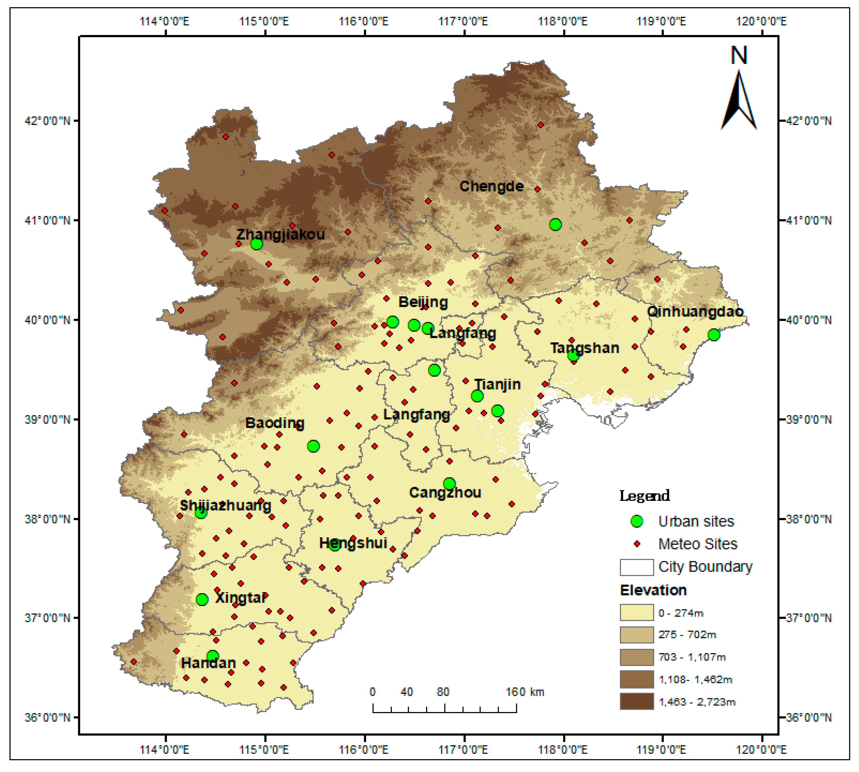
2. Materials and Methods

The Beijing–Tianjing–Hebei urban agglomeration region, located in the Huabei plain of northern China, is one of the most important economic zones in China. This region has undergone rapid urbanization since the 1990s. There are 13 cities in the BTH region with the urbanization rates varying from 47% to 87% in 2015. As

Table 1. Population density and gross domestic product (GDP) information for Beijing–Tianjing–Hebei (BTH) cities in 2015 (Data came from the statistical yearbook of Hebei province, Beijing city and Tianjin city, for example: http://tjj.beijing.gov.cn/English).

City Name	Population Density (Person/km2)	GDP (Billion RMB Yuan)
Baoding	520.7	344.9
Beijing	1313	2800
Cangzhou	519.2	364.3
Chengde	89.3	146.5
Handan	781.5	337.9
Hengshui	501.9	152.3
Langfang	711.1	288.1
Qinhuangdao	394.4	150.1
Shijiazhuang	761.5	617.7
Tangshan	557.8	653
Tianjin	861	1859.5
Xingtai	586.7	209.1
Zhangjiakou	120.1	142.7

shows, the varied population density from 89.3 to 1313 and the different economic condition indicate the unbalanced developments among the 13 cities. As the first two developed cities, Beijing and Tianjin had the first two population density and gross domestic product (GDP) and accordingly presented the most significant UHI effects in BTH region [23].

As per the up to date Köppen–Geiger climate classification [24], the BTH region belongs to monsoon-influenced hot-summer humid continental climate. According to statistical yearbook, from 1986–2015, the annual average precipitation of BTH region is 540 mm, the average summer maximum temperature is 31.5 °C, and the average winter minimum temperature is –7.1 °C

Mountains and hills are distributed in the north and part of the west, the basins next to the northeast highland and plains are extensively distributed across the central and southeastern areas (Figure 1). Zhangjiakou and Chengde were considered mountainous cities in this study because 17 of 23 (74%) sites’ altitudes are greater than 700 m with rugged terrains. The maximum altitude in BTH is 2882 m, the plain counts 45% of total area in BTH region and the mean altitude of plain is <100 m. Tianjin, Tangshan and Qinhuangdao are adjacent to the Bohai sea while other cities are inland cities.

Data and Methods

The field data of 174 sites were provided by the National Meteorological Information Center (NMIC, https://data.cma.cn/). The air temperature was recorded at the height of 2 m above the ground. The abnormal values (assigned 9999) in the field dataset have been excluded. The yearly mean air temperature was averaged based on the daily mean temperature, and the maximum and minimum air temperatures were extracted through daily maximum and minimum temperatures throughout a year. Sites located in the urban areas were identified as the urban sites while the others located outside the urban areas were grouped as rural sites. Except Beijing (3 urban sites) and Tianjin (2 urban sites), there was only 1 urban site in other cities. The observations of urban sites in Beijing and Tianjin were averaged, respectively. A total of 16 urban sites were chosen, and 158 rural sites were identified.

According to the site locations, maximum, minimum and mean temperatures were extracted based on latitude/longitude (lat/lon) points. To match with the remote sensing data, the time scope of this study was from 2001 to 2015. The five-year moving average method was employed to smooth the variant field temperatures (Equation (1)):

$${\mathrm{T}}_{\mathrm{MA}}=\frac{{\mathrm{T}}_{\mathrm{k}-2}+{\mathrm{T}}_{\mathrm{k}-1}+{\mathrm{T}}_{\mathrm{k}}+{\mathrm{T}}_{\mathrm{k}+1}+{\mathrm{T}}_{\mathrm{k}+2}}{5}$$

(1)

${\mathrm{T}}_{\mathrm{MA}}$ is the averaged value, ${\mathrm{T}}_{\mathrm{k}-2}\dots {\mathrm{T}}_{\mathrm{k}}\dots {\mathrm{T}}_{\mathrm{k}+2}$ indicates the time series of 5-year temperatures. The Moderate Resolution Imaging Spectroradiometer (MODIS) LST product (MOD11A2 from the Terra satellite) was utilized to extract the surface UHI values and to compare with the SAT. The up-to-date (version 6) 8-day composite 1 km data were downloaded from https://earthdata.nasa.gov/. The Terra MODIS transits at local time of 10:30 AM and 10:30 PM, which produced the daytime and nighttime LST, respectively. Mean LST was averaged between daytime and nighttime LST retrievals, maximum and minimum LST values were extracted from daytime and nighttime layers of the LST product, respectively. The images were averaged from 8-day to yearly with arithmetic mean method. The failed retrieval pixels (Fill value) were assigned as ‘NoData’ by python and were excluded.

To match with the locations of field observations, the LST values in urban and rural areas were extracted according to the field site locations. In particular, to avoid the potential erratic maximum LST values, we sorted the extracted pixels within each year (there were 44 images per year) and averaged the first 5 maximum values as the maximum temperature in the current year, which produced the average max temperature for 40 days (8 day × 5).

Linear fitting, histogram statistics and trend analysis were combined to evaluate the temporal tendencies of LST and SAT. The fitting slope (°C/year) was used as the main indicator to compare the temporal trends. The linear fitting model was utilized and analysis of variance (ANOVA) was conducted in Originpro software. The coefficient of determination (R²) and root-mean-square errors (RMSE) were used to evaluate the correlations and the discreteness of regression, respectively. The UHI effects were calculated by absolute differences of urban and rural site temperatures. The nighttime UHI was calculated from the minimum temperature values, the daytime mean and maximum UHI intensities can be characterized by mean and maximum temperatures, respectively. The coefficient of variation (CV) measured the dispersion of time series data, and was calculated to distinguish the potential impact factors. The effects of topography and parameter stability were evaluated by CV values between LST and SAT for all the cities.

3. Results

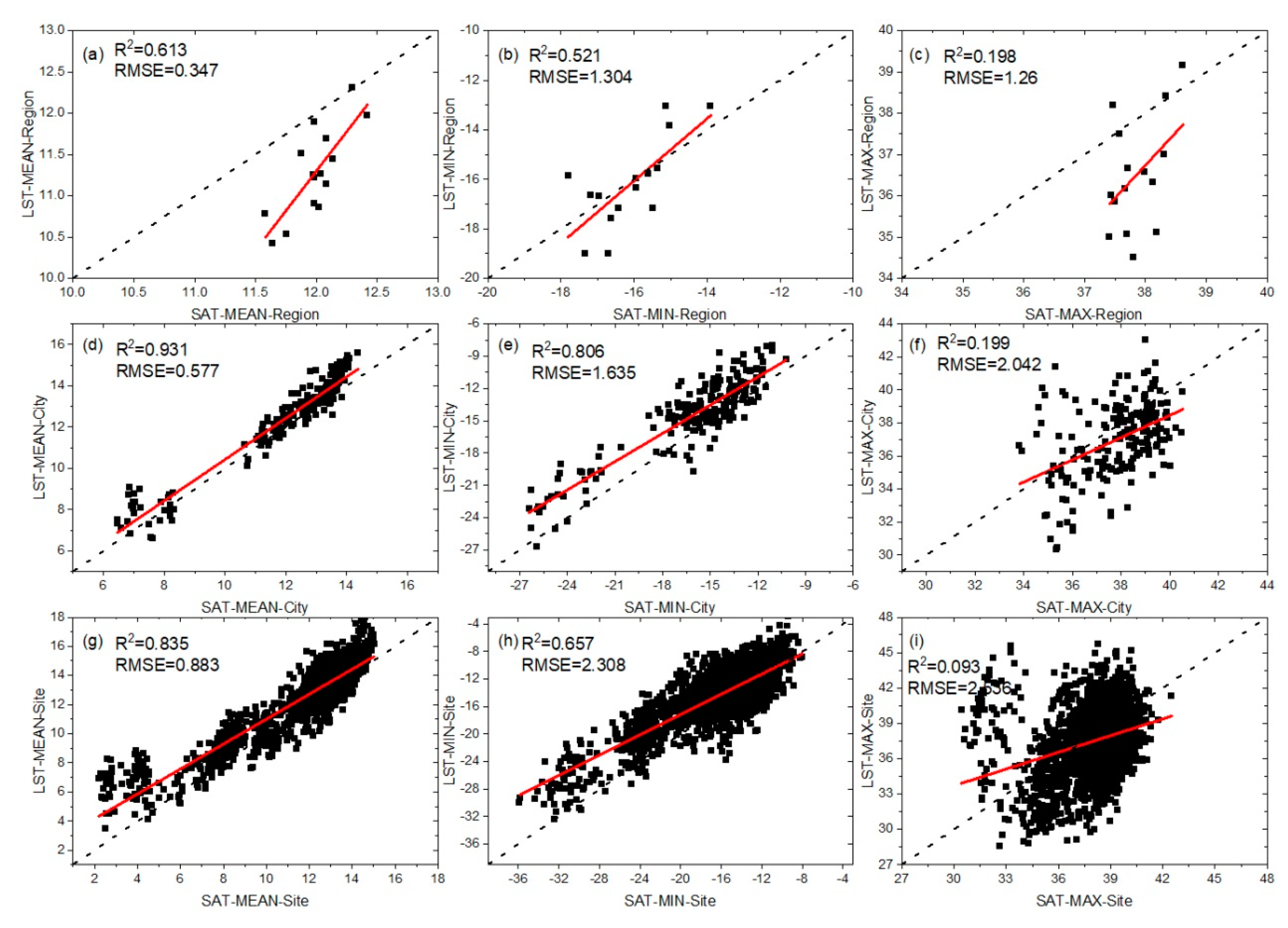
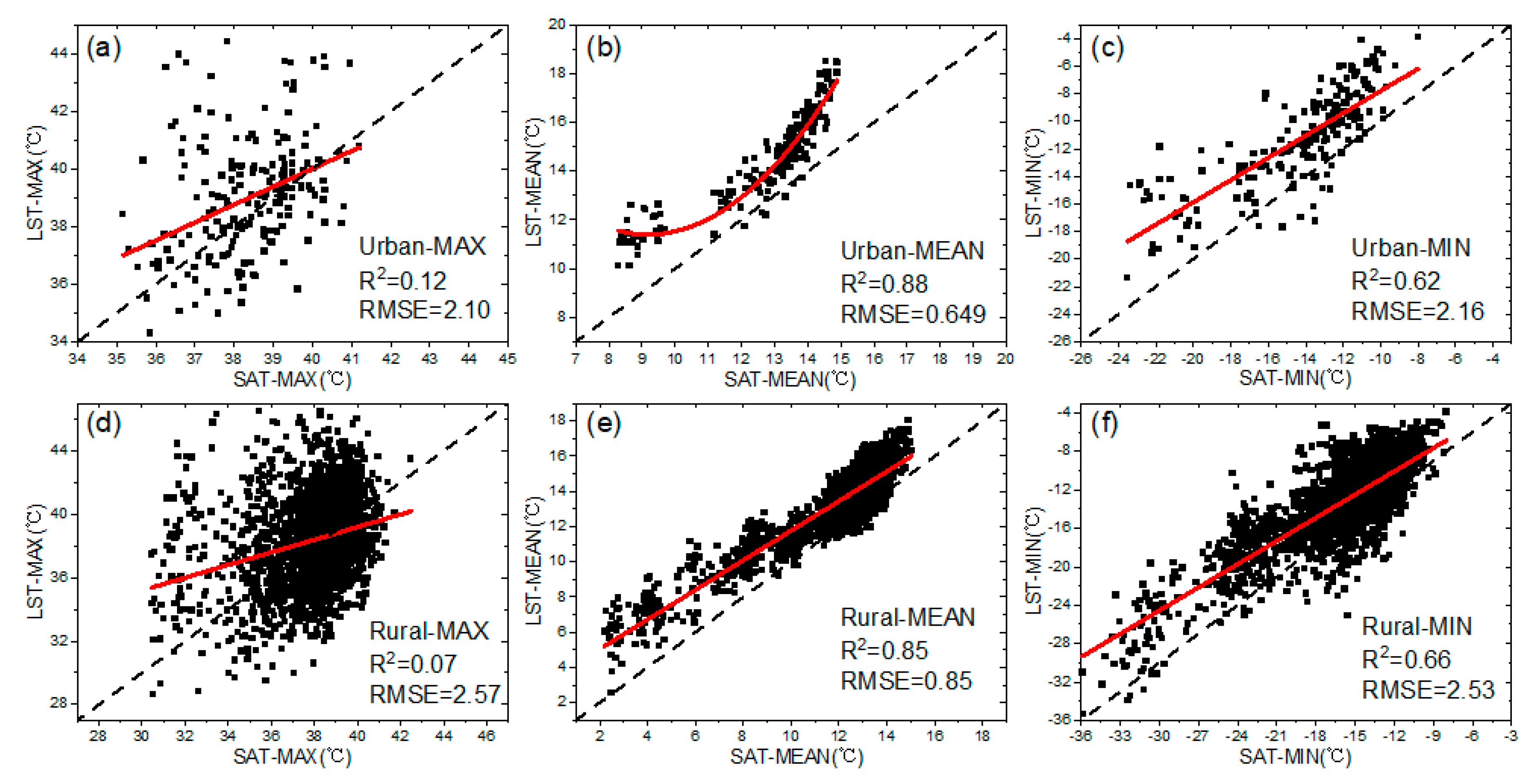
3.1. Regression Characteristics between Land Surface Temperature (LST) and Surface Air Temperature (SAT)

The regression fittings of minimum, mean and maximum temperatures were compared between SAT and LST (Figure 2). The columns in the figure indicate mean, minimum and maximum temperatures, and the rows indicate the regional, city and site scales. The best agreements were observed for yearly mean temperature, with the highest determination coefficients (R² = 0.613, 0.931 and 0.835) and the lowest fitting discreteness (RMSE = 0.347, 0.577 and 0.883) at region, city and site scales (Figure 2a,d,g), followed by the yearly minimum temperatures (Figure 2b,e,h). Yearly maximum temperatures show the lowest determination coefficients (R² = 0.198, 0.199 and 0.099) and high discreteness (RMSE = 1.26, 2.042 and 2.536) (Figure 2c,f,i). The highly variations of maximum LST values and relatively concentrated field maximum air temperatures combined to produce the poor fittings. Although the thermal environment may contribute to the maximum temperature, the climatic impacts were thought as the main reason that produced the highly variations of the maximum temperatures for both LST and SAT [25].

Among the three scales, LST and SAT show the best consistency at the city scale, with determination coefficients R² of 0.93 and 0.81 for the mean and minimum temperatures, respectively (Figure 2d,e); Moderate results were observed at the site scale, with R² of 0.84 and 0.66 for the mean and minimum temperatures (Figure 2g,h). It was the lowest at the regional scale, with R² below 0.65 for all three temperatures.

The absolute values between SAT and LST were compared via 1:1 lines in Figure 2. At the regional scale, SAT was higher than LST with more scatter points at the side of SAT for yearly mean and maximum temperatures (Figure 2a,c). At the city scale, more fitting points showed higher values in LST than those in SAT for yearly mean and minimum temperatures, and more points in SAT were higher than LST for yearly maximum temperature. At the site scale, most LST values were higher than SAT in yearly mean and minimum temperatures, and SAT was higher than LST in maximum temperatures. Some poorly fitted points, which belong to the mountainous Zhangjiakou city (Figure 2g,i), caused low coefficients and high discreteness of fittings, which hints at the large discrepancies between LST and SAT over the rugged terrains.

The urban and rural sites were separated and the relations of LST and SAT were regressed in Figure 3. Similar fitting patterns were observed between urban and rural sites for maximum (Figure 3a,d) and minimum temperatures (Figure 3c,f). The minimum temperature performed better fittings than the maximum temperature in both urban and rural sites. The mean temperature in urban sites presented the exponential pattern between LST and SAT with the higher fitting coefficient (Figure 3b, R² = 0.88) and lower discreteness (RMSE = 0.649) than rural mean temperature (Figure 3e). LST increased faster than SAT when the mean air temperature exceeds 11 °C in urban sites, which indicates the higher surface temperature than the air temperature in warmer urban environments. In Figure 3b, mean LST kept around 11 °C when SAT increased from 8 °C to 10 °C. These scattered points belong to mountainous Zhangjiakou city and part of Chengde city. This insensitive performance indicated the uncertainties of mean LST in mountainous areas.

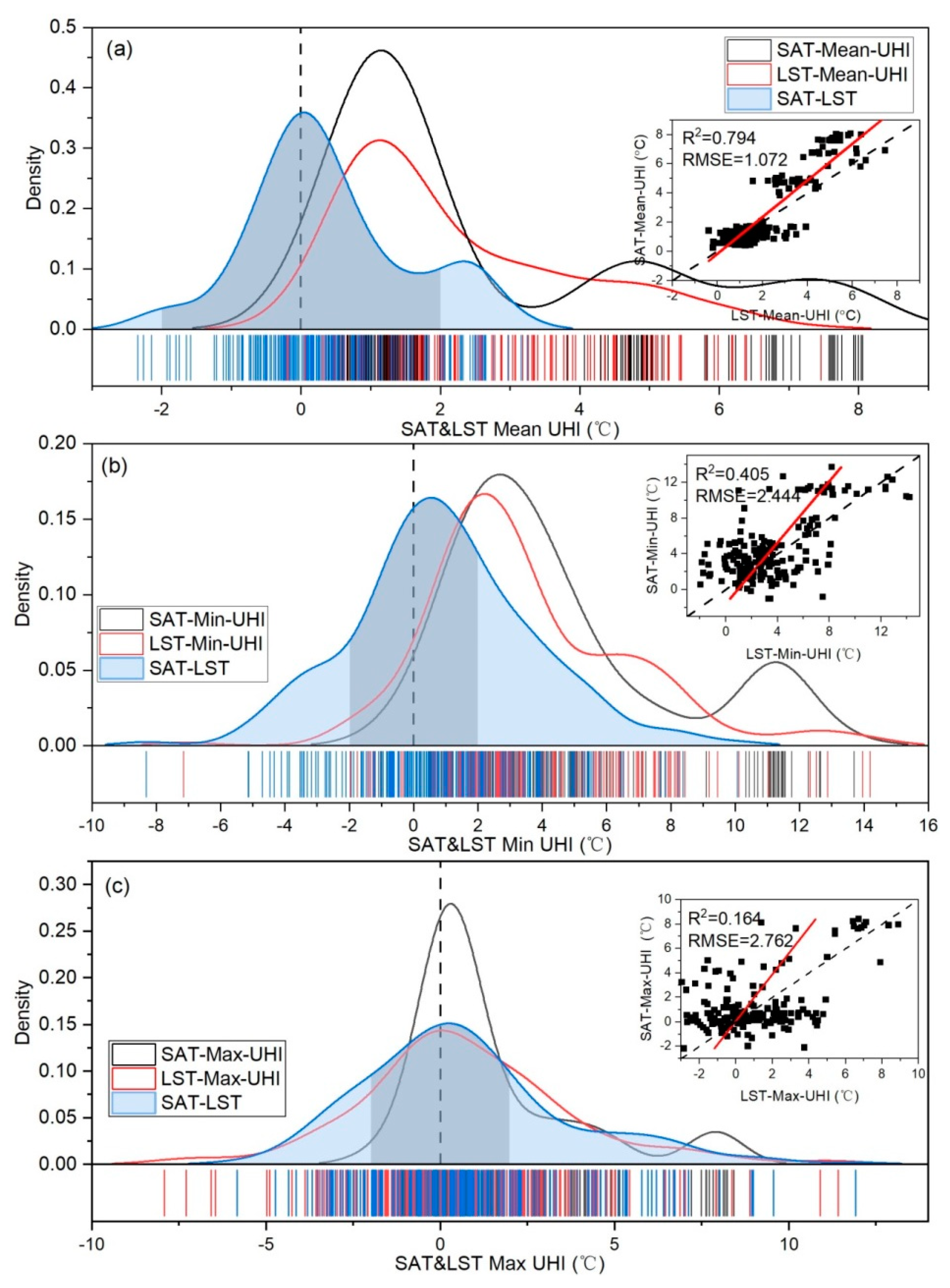
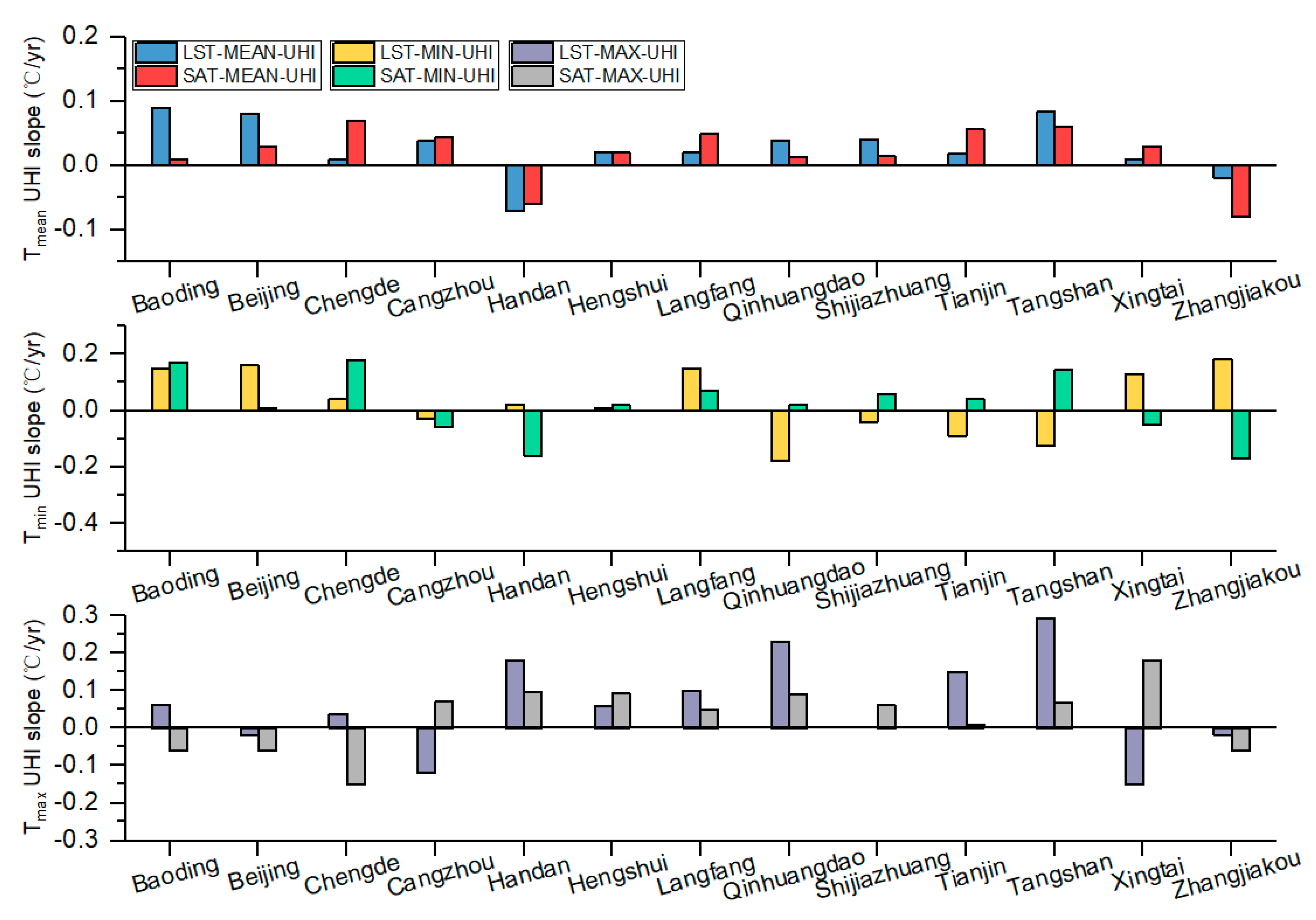
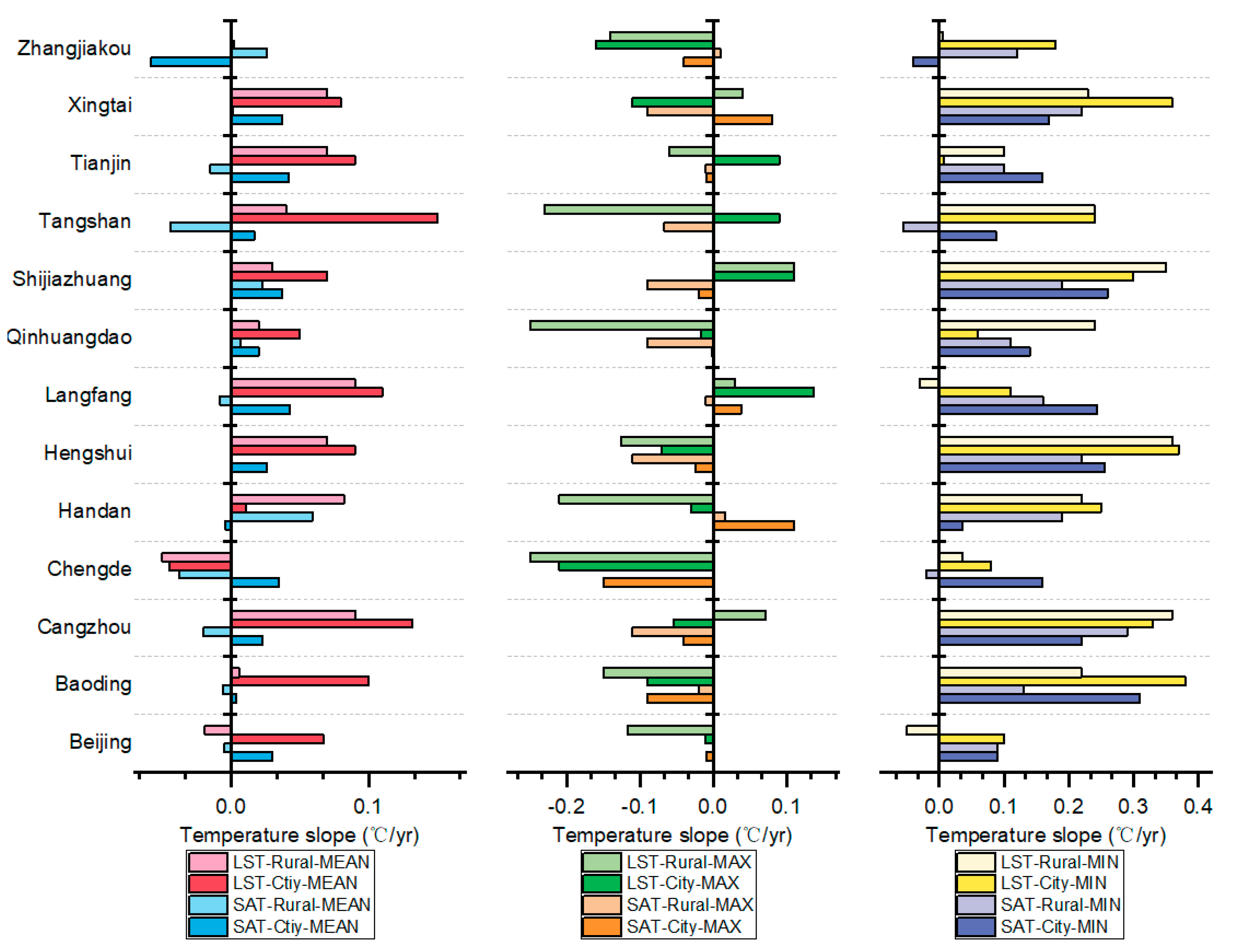
3.2. Urban Heat Island (UHI) Consistencies between LST and SAT

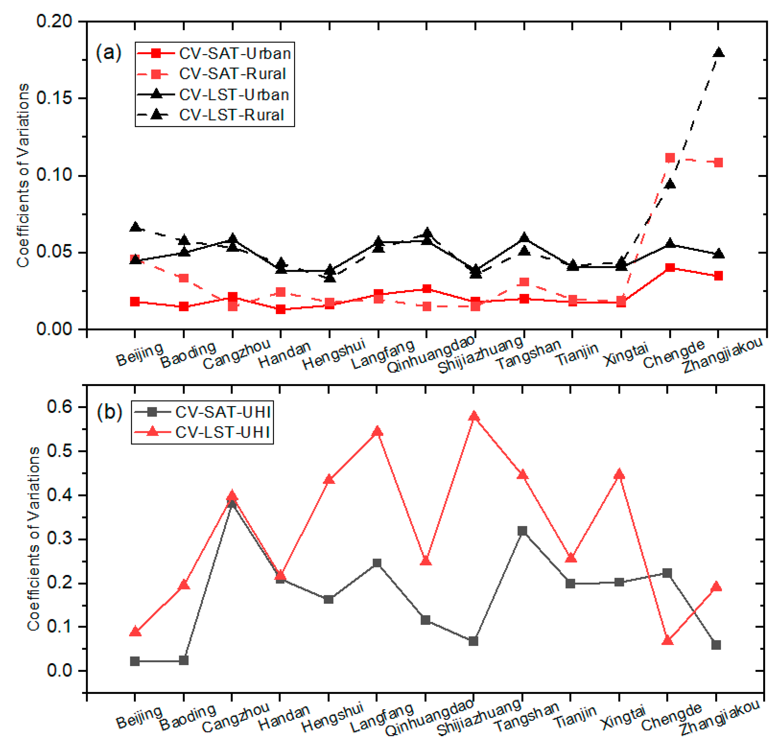
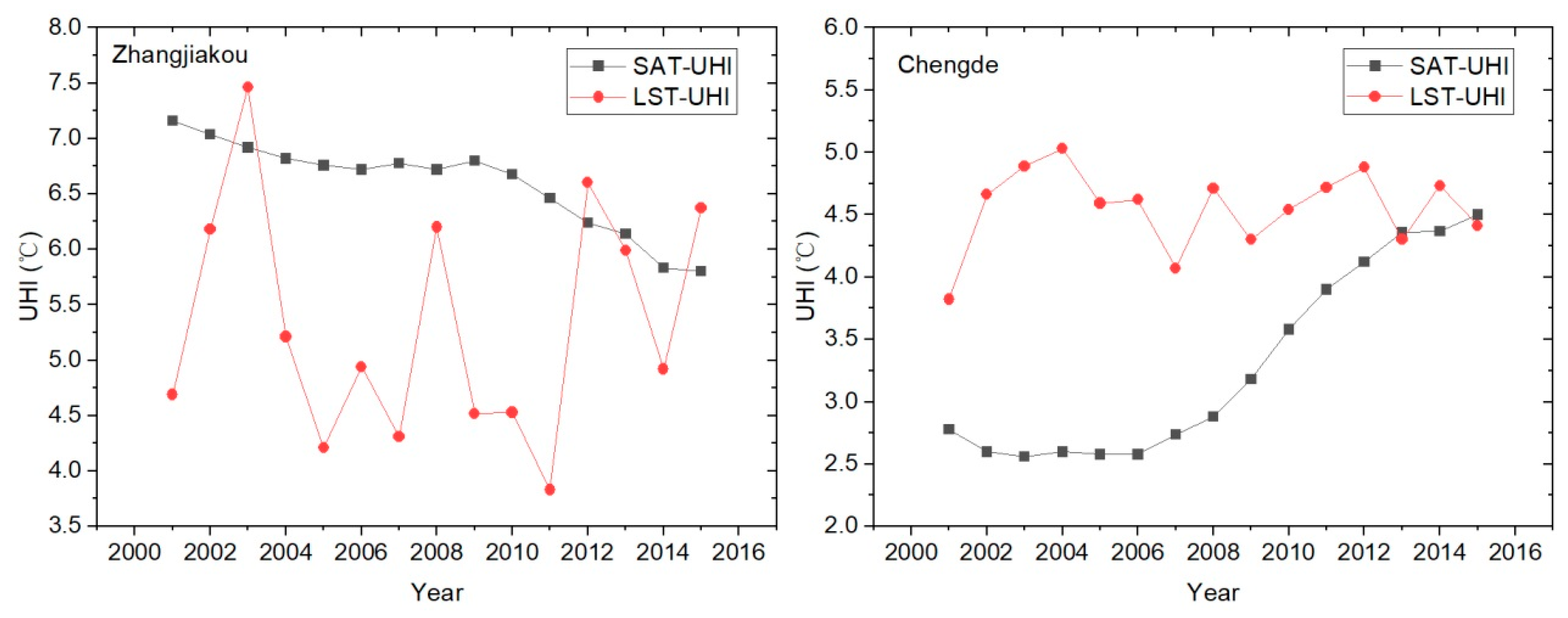
Statistical Distributions of UHI Values

The UHI intensities of LST and SAT were calculated and are illustrated as the density histograms in Figure 4 as well as the differences between SAT-UHI and LST-UHI. The linear fittings between LST-UHI and SAT-UHI of each temperature type are shown as the subplots.

For mean temperature (Figure 4a), the general statistical consistency between LST-UHI and SAT-UHI was observed (R² = 0.794, RMSE = 1.072). SAT presented broader UHI ranges than LST. SAT showed that 45% of urban sites are 1 to 2 °C higher than rural sites while the proportion was 30% for LST. Both the Gaussian-like distribution and the scatter plot indicated the large discrepancies between LST and SAT when UHI > 4 °C. In terms of the UHI histogram, many UHI values fell between –2 °C to 2 °C, which accounted for 84.1 % of the total UHI values. SAT got larger UHI range with more values aggregated to 0 to 2 °C. SAT presented higher UHI values than LST over some sites, which belong to the mountainous cities Zhangjiakou and Chengde.

For minimum temperature (Figure 4b), more obvious discreteness and lower fitting accuracy were observed (R² = 0.405, RMSE = 2.444). The peaks of histograms were also different between LST-UHI and SAT-UHI. The peak of SAT-UHI was 3 °C with 18% UHI values while the peak of LST-UHI was 2 °C with 16% UHI values. A broader range [–6, 6] of differences between SAT and LST for minimum temperature was presented, which implies the significant disparities between SAT and LST in denoting the UHI. Only 55.3% of minimum UHI values fell in the range of [–2, 2 °C].

The maximum temperature (Figure 4c) performed the lowest consistency between LST-UHI and SAT-UHI with the lowest fitting results (R² = 0.164, RMSE = 2.762). Nearly 28% of SAT-UHI values and 13% of LST-UHI values were close to 0 °C, respectively. Moreover, there were 56.9 °C % LST-UHI values greater than 0 °C and the percentage was 77.4% for SAT-UHI. The differences between SAT and LST of maximum temperature also presented the broad range [–5, 5 °C] and only 58.4% of differences UHI values fell in the [–2, 2°C]. From the subplot of Figure 4c, the overestimations were obvious for LST-UHI when SAT-UHI was nearby 0 °C.

To further compare the trends of LST-UHI and SAT-UHI, the slopes of temporal UHI were calculated in Figure 5. The trend consistency was observed in mean temperature between LST-UHI and SAT-UHI. For mean temperature (Figure 5a), both LST and SAT show increasing UHI tendencies for most of the cities, suggesting both of them could capture the accelerated urbanization effects. However, discrepancies of slopes were found in most of the cities. LST-UHI shows higher increasing slopes than SAT-UHI in 6 cities, which were Beijing, Baoding, Shijiazhuang, Handan, Qinhuangdao and Tangshan. Baoding recorded the largest discrepancy of trend slopes between LST-UHI (0.09) and SAT-UHI (0.01). Another 6 cities, Tianjin, Chengde, Cangzhou, Langfang, Xingtai and Zhangjiakou showed higher SAT-UHI trends. Hengshui city presents the same slopes between LST-UHI and SAT-UHI (0.02).

In addition to the slope values, the disparities of trend direction were observed in maximum and minimum temperatures (Figure 5b,c). The opposite UHI trends were observed in 7 of 13 cities for minimum temperature and in 5 of 13 cities for maximum temperature. Therefore, the inconsistencies of temporal trends between LST-UHI and SAT-UHI hinted that more considerations are needed to conduct further applications by using minimum and maximum temperatures directly.

Figure 6 illustrates the temperature slopes of LST and SAT in city and rural sites, which is used to explain the variations of UHI tendencies in Figure 5. For mean temperature in most of the cities, both urban and rural temperatures showed increasing tendencies and most of urban sites have higher increasing trends than rural sites. For maximum temperature, the increasing UHI slopes in Figure 5 resulted from the decreased rural maximum temperatures for both LST and SAT, and which also presents the decreasing maximum temperature over the entire BTH region. In addition, the minimum temperature slopes in urban and rural areas have increased significantly, which indicates regional climate warming.

3.3. Effects of Parameter Stability and Topography

LST stability and the topography combined impact the relationships between LST and SAT. Hence, we further conducted examinations of CV for temperatures and UHI values to distinguish the roles of these two factors (Figure 7). Both urban and rural LST values presented higher temporal variabilities than SAT values in Figure 7a, which caused the higher variabilities of derived LST-UHI than SAT-UHI values. Therefore, the temporal instability of LST was the main reason that caused the larger uncertainties of LST-UHI than SAT among most of cities (Figure 7b). This result implies that it is better to use SAT as the reference to ensure the reliability of the LST-derived UHI in indicating the urbanization thermal effects.

Both SAT and LST in mountainous areas were affected significantly by the topography (Figure 7a). Much higher variabilities (CV) in mountainous rural sites of Chengde and Zhangjiakou cities were observed. Even for the urban sites, the CV values of SAT in mountainous cities were higher than cities located in plain areas. Beijing also presented the topography effects because several rural sites were located on the northern mountain, which also showed higher variabilities than urban site in both LST and SAT. Given the much higher CV values, we concluded that topography is an important factor that influences the relationships between LST and SAT. Cloud and direct solar insolation may contribute to the variability in rugged terrains [12].

The temporal UHI values were illustrated to further explain the high CV of LST and SAT in mountainous areas (Figure 8). The lower variations of UHI in Chengde and Zhangjiakou were observed in Figure 7b. The temporal changes of UHI derived from LST and SAT were presented in Figure 8 to explain the fluctuations in Figure 7b. The smooth trends of SAT-UHI and the significant variability of LST-UHI were observed in both cities. The higher CV value for SAT in Chengde came from the obvious increasing SAT-UHI values, which was due to the decreased rural temperatures in Chengde (not presented in the paper). For the other Zhangjiakou city, the lower CV value of SAT came from the mild decreasing of SAT-UHI, which was mainly due to the slowly increased rural temperatures (not presented in this paper). Hence, how the rugged terrains affect LST and SAT still need more research.

4. Discussion

It was thought that the ‘LST-SAT’ relationship can be affected by urban environment via the extensive impervious surface in [26]. However, we found the fittings between LST and SAT in urban sites also had high determination coefficients (R² = 0.794) through the exponential model, which indicated that the urban environment may modify the LST-SAT relationship, but not to depreciate the close connections between LST and SAT. As to the UHI, the faster increasing urban mean LST in Figure 3 will not definitely cause the higher UHI intensities than SAT due to the higher LST values in rural areas.

In addition to the CV variations of topography effects, the weaker temporal trends for LST-UHI than SAT-UHI in mountainous Chengde and Zhangjiakou also provided evidence for the complex terrain effects on the LST-UHI (Figure 5 and Figure 6). Weaker effects caused by the complex terrain on the relationships between LST and SAT have been reported [16,17] and confirmed in this study. Furthermore, we found that the rugged terrains impacted the temporal UHI effects through the large uncertainties of LST. The poor fitting results for the maximum temperature were different from some previous studies [5,7]. In this paper, although we used the time series average method to smooth the maximum LST, strong temporal variations were still observed. The various types of underlying surfaces and the fluctuations of maximum temperature are the potential reasons for the poor fitting coefficients. Therefore, we argue that the LST values need more examination especially for minimum and maximum values.

Several studies believed that LST can represent the characteristics of air temperature through diurnal [27] and monthly [12] direct comparisons, but the temporal representativeness of LST to the distribution of terrestrial heat flux was doubted in [28], which produced the SAT by hierarchical Bayesian method from MODIS LST. According to our evaluations, high connections and the same trends for UHI effects of mean temperature have been found between LST and SAT, but the large discrepancies of UHI magnitudes have been observed temporally, which were caused by the temporal instability of LST values and the complex terrains. Hence, the intrinsic differences between LST and SAT told that the LST results should be carefully extended as the attributes of SAT in urban thermodynamic research.

In addition, climate zones, cloud, solar irradiance, vegetation cover and seasonality variations of urban and rural environments are potential factors that may affect the UHI trends between LST and SAT. The daily and seasonal UHI characteristics between LST and SAT may have different performance because the yearly results will smooth the daily and seasonality attributes. This study hinted at further research directions to explore the mechanism of variations of urban heat island.

5. Conclusions

For evaluating the UHI effects credibly, the temporal characteristics between LST and SAT need more examination. In this paper, yearly mean, maximum and minimum temperatures were extracted to assess the consistencies between LST and SAT. The paper found: (1) LST and SAT obtained the best regression fittings (R² = 0.931) from mean temperature at the city scale. LST and SAT had similar fitting results in urban sites and rural sites. LST increase faster than SAT in warmer urban environments making it less useful for UHI calculation and prediction. (2) As for the UHI effects, good statistical consistency between LST-UHI and SAT-UHI was observed only in mean temperature (R² = 0.794). Lower and discrete fitting results were shown in minimum (R² = 0.405) and maximum (R² = 0.164) temperatures. There are 84.1% of different values between SAT-UHI and LST-UHI in the range of [–2, 2°C] while the proportions were only 55.3% and 58.4% for minimum and maximum, respectively. (3) Same UHI temporal trends were found in mean temperatures between LST and SAT, but highly different trend slopes hinted the inadequacy to reveal the UHI variations only from LST, especially for nighttime (minimum) and daytime (maximum) UHI intensities. The opposite trends between LST-UHI and SAT-UHI showed the limited reliability of LST in indicating the long term variations of urban thermal effects. (4) The temporal fluctuations of LST caused the higher uncertainties of LST-UHI than SAT-UHI. The rugged terrain was an important factor to affect the UHI intensities for both LST and SAT. In this paper, we suggest that the SAT should be combined with LST to present more credible UHI characteristics. This paper can be a reference for understanding the UHI effects at different scales and will help in understanding of the connections between surface and near-surface temperatures in various natural conditions.

References

1. Ziter, C.D.; Pedersen, E.J.; Kucharik, C.J.; Turner, M.G. Scale-dependent interactions between tree canopy cover and impervious surfaces reduce daytime urban heat during summer. Proc. Natl. Acad. Sci. USA 2019, 116, 7575–7580. [Google Scholar] [CrossRef] [PubMed] [Green Version]
2. Manoli, G.; Fatichi, S.; Schläpfer, M.; Yu, K.; Crowther, T.W.; Meili, N.; Burlando, P.; Katul, G.G.; Bou-Zeid, E. Magnitude of urban heat islands largely explained by climate and population. Nature 2019, 573, 55–60. [Google Scholar] [CrossRef] [PubMed]
3. Zhou, D.; Zhang, L.; Li, D.; Huang, D.; Zhu, C. Climate–vegetation control on the diurnal and seasonal variations of surface urban heat islands in China. Environ. Res. Lett. 2016, 11, 74009. [Google Scholar] [CrossRef]
4. Rao, Y.; Liang, S.; Wang, D.; Yu, Y.; Song, Z.; Zhou, Y.; Shen, M.; Xu, B. Estimating daily average surface air temperature using satellite land surface temperature and top-of-atmosphere radiation products over the Tibetan Plateau. Remote Sens. Environ. 2019, 234, 111462. [Google Scholar] [CrossRef]
5. Mildrexler, D.J.; Zhao, M.; Running, S.W. A global comparison between station air temperatures and MODIS land surface temperatures reveals the cooling role of forests. J. Geophys. Res. 2011, 116, 116. [Google Scholar] [CrossRef]
6. Tomlinson, C.J.; Chapman, L.; Thornes, J.E.; Baker, C.J.; Prieto-Lopez, T. Comparing night-time satellite land surface temperature from MODIS and ground measured air temperature across a conurbation. Remote Sens. Lett. 2012, 3, 657–666. [Google Scholar] [CrossRef]
7. Hadria, R.; Benabdelouahab, T.; Mahyou, H.; Balaghi, R.; Bydekerke, L.; El Hairech, T.; Ceccato, P. Relationships between the three components of air temperature and remotely sensed land surface temperature of agricultural areas in Morocco. Int. J. Remote Sens. 2018, 39, 356–373. [Google Scholar] [CrossRef]
8. Huang, R.; Zhang, C.; Huang, J.; Zhu, D.; Wang, L.; Liu, J. Mapping of Daily Mean Air Temperature in Agricultural Regions Using Daytime and Nighttime Land Surface Temperatures Derived from TERRA and AQUA MODIS Data. Remote Sens. 2015, 7, 8728–8756. [Google Scholar] [CrossRef] [Green Version]
9. Cheval, S.; Dumitrescu, A. The summer surface urban heat island of Bucharest (Romania) retrieved from MODIS images. Theor. Appl. Climatol. 2015, 121, 631–640. [Google Scholar] [CrossRef]
10. Shiflett, S.A.; Liang, L.L.; Crum, S.M.; Feyisa, G.L.; Wang, J.; Jenerette, G.D. Variation in the urban vegetation, surface temperature, air temperature nexus. Sci. Total Environ. 2017, 579, 495–505. [Google Scholar] [CrossRef]
11. Azevedo, J.; Chapman, L.; Muller, C. Quantifying the Daytime and Night-Time Urban Heat Island in Birmingham, UK: A Comparison of Satellite Derived Land Surface Temperature and High Resolution Air Temperature Observations. Remote Sens. 2016, 8, 153. [Google Scholar] [CrossRef] [Green Version]
12. Good, E.J.; Ghent, D.J.; Bulgin, C.E.; Remedios, J.J. A spatiotemporal analysis of the relationship between near-surface air temperature and satellite land surface temperatures using 17 years of data from the ATSR series. J. Geophys. Res. Atmos. 2017, 122, 9185–9210. [Google Scholar] [CrossRef]
13. Sheng, L.; Tang, X.; You, H.; Gu, Q.; Hu, H. Comparison of the urban heat island intensity quantified by using air temperature and Landsat land surface temperature in Hangzhou, China. Ecol. Indic. 2017, 72, 738–746. [Google Scholar] [CrossRef]
14. Xiong, Y.; Chen, F. Correlation analysis between temperatures from Landsat thermal infrared retrievals and synchronous weather observations in Shenzhen, China. Remote Sens. Appl. Soc. Environ. 2017, 7, 40–48. [Google Scholar] [CrossRef]
15. Schwarz, N.; Schlink, U.; Franck, U.; Großmann, K. Relationship of land surface and air temperatures and its implications for quantifying urban heat island indicators—An application for the city of Leipzig (Germany). Ecol. Indic. 2012, 18, 693–704. [Google Scholar] [CrossRef]
16. Lin, X.; Zhang, W.; Huang, Y.; Sun, W.; Han, P.; Yu, L.; Sun, F. Empirical Estimation of Near-Surface Air Temperature in China from MODIS LST Data by Considering Physiographic Features. Remote Sens. 2016, 8, 629. [Google Scholar] [CrossRef] [Green Version]
17. Mutiibwa, D.; Strachan, S.; Albright, T. Land Surface Temperature and Surface Air Temperature in Complex Terrain. IEEE JSTARS 2015, 8, 4762–4774. [Google Scholar] [CrossRef]
18. Pepin, N.C.; Maeda, E.E.; Williams, R. Use of remotely sensed land surface temperature as a proxy for air temperatures at high elevations: Findings from a 5000  m elevational transect across Kilimanjaro. J. Geophys. Res. Atmos. 2016, 121, 9910–9998. [Google Scholar] [CrossRef] [Green Version]
19. Gallo, K.P.; McNab, A.L.; Karl, T.R.; Brown, J.F.; Hood, J.J.; Tarpley, J.D. The use of NOAA AVHRR data for assessment of the urban heat island effect. J. Appl. Meteorol. 1993, 32, 899–908. [Google Scholar] [CrossRef] [Green Version]
20. Streutker, D.R. A remote sensing study of the urban heat island of Houston, Texas. Int. J. Remote Sens. 2002, 23, 2595–2608. [Google Scholar] [CrossRef]
21. Schwarz, N.; Lautenbach, S.; Seppelt, R. Exploring indicators for quantifying surface urban heat islands of European cities with MODIS land surface temperatures. Remote Sens. Environ. 2011, 115, 3175–3186. [Google Scholar] [CrossRef]
22. Gao, Z.; Hou, Y.; Chen, W. Enhanced sensitivity of the urban heat island effect to summer temperatures induced by urban expansion. Environ. Res. Lett. 2019, 14, 094005. [Google Scholar] [CrossRef] [Green Version]
23. Li, M.; Wang, T.; Xie, M.; Zhuang, B.; Li, S.; Han, Y.; Cheng, N. Modeling of urban heat island and its impacts on thermal circulations in the Beijing–Tianjin–Hebei region, China. Theor. Appl. Climatol. 2017, 128, 999–1013. [Google Scholar] [CrossRef]
24. Beck, H.E.; Zimmermann, N.E.; McVicar, T.R.; Vergopolan, N.; Berg, A.; Wood, E.F. Present and future Köppen-Geiger climate classification maps at 1-km resolution. Sci. Data 2018, 5, 180214. [Google Scholar] [CrossRef] [PubMed] [Green Version]
25. Wang, J.; Huang, B.; Fu, D.; Atkinson, P.M.; Zhang, X. Response of urban heat island to future urban expansion over the Beijing–Tianjin–Hebei metropolitan area. Appl. Geogr. 2016, 70, 26–36. [Google Scholar] [CrossRef]
26. Zhao, S.; Zhou, D.; Liu, S. Data concurrency is required for estimating urban heat island intensity. Environ. Pollut. 2016, 208, 118–124. [Google Scholar] [CrossRef]
27. Cheval, S.; Dumitrescu, A.; Bell, A. The urban heat island of Bucharest during the extreme high temperatures of July 2007. Theor. Appl. Climatol. 2009, 97, 391–401. [Google Scholar] [CrossRef]
28. Lu, N.; Liang, S.; Huang, G.; Qin, J.; Yao, L.; Wang, D.; Yang, K. Hierarchical Bayesian space-time estimation of monthly maximum and minimum surface air temperature. Remote Sens. Environ. 2018, 211, 48–58. [Google Scholar] [CrossRef]
Figure 1. The distribution of meteorological sites and the terrain of the study area.
Remotesensing 12 01271 g001
Figure 2. (ai) Regressions between surface air temperature (SAT) and land surface temperature (LST) at regional, city and site scales based on the yearly data (red and dotted lines indicate the fitting and 1:1 line, respectively).
Remotesensing 12 01271 g002
Figure 3. (af) Comparison of LST-SAT regressions between urban and rural sites.
Remotesensing 12 01271 g003
Figure 4. Statistical distributions and linear fittings between LST-UHI (urban heat island) and SAT-UHI for mean (a), minimum (b) and maximum (c) temperatures. Blue area means the differences between SAT-UHI and LST-UHI, gray shadows means the proportions of differences within the [–2, 2] range. Dotted lines are references of 0.0 for X axis and 1:1 line for subplots. The vertical dotted line indicated the zero reference.
Remotesensing 12 01271 g004
Figure 5. The trends of UHI slopes derived from LST and SAT.
Remotesensing 12 01271 g005
Figure 6. Trend comparisons of LST and SAT temperatures.
Remotesensing 12 01271 g006
Figure 7. (a,b) The coefficients of variation (CV) of mean temperatures and UHI values.
Remotesensing 12 01271 g007
Figure 8. Temporal changes of LST-UHI and SAT-UHI in mountainous Chengde and Zhangjiakou cities.
Remotesensing 12 01271 g008