A Refined Four-Stream Radiative Transfer Model for Row-Planted Crops

Abstract

In modeling the canopy reflectance of row-planted crops, neglecting horizontal radiative transfer may lead to an inaccurate representation of vegetation energy balance and further cause uncertainty in the simulation of canopy reflectance at larger viewing zenith angles. To reduce this systematic deviation, here we refined the four-stream radiative transfer equations by considering horizontal radiation through the lateral “walls”, considered the radiative transfer between rows, then proposed a modified four-stream (MFS) radiative transfer model using single and multiple scattering. We validated the MFS model using both computer simulations and in situ measurements, and found that the MFS model can be used to simulate crop canopy reflectance at different growth stages with an accuracy comparable to the computer simulations (RMSE < 0.002 in the red band, RMSE < 0.019 in NIR band). Moreover, the MFS model can be successfully used to simulate the reflectance of continuous (RMSE = 0.012) and row crop canopies (RMSE < 0.023), and therefore addressed the large viewing zenith angle problems in the previous row model based on four-stream radiative transfer equations. Our results demonstrate that horizontal radiation is an important factor that needs to be considered in modeling the canopy reflectance of row-planted crops. Hence, the refined four-stream radiative transfer model is applicable to the real world.

1. Introduction

Canopy reflectance modeling for row-planted crops is a hot topic in quantitative remote sensing of vegetation, which is promising for developing physics-based methods to estimate canopy biophysical parameters [1,2,3,4]. In the inversion of remote sensing, the efficiency of the inversion is closely related to the calculation time and accuracy of the model [5]. In general, the physical modeling methods can be separated into three categories, namely geometric optical, computer simulation, and radiative transfer methods [5]. In these modeling techniques, compared with geometric optics that only consider surface reflectance [6,7], radiative transfer considers the leaf inclination angle distribution function (LADF) from a statistical perspective inside the canopy [8,9]. Then, based on LADF, the volume scattering inside the canopy can be accurately described [10], thereby improving the accuracy of the reflectance. Simultaneously, compared with computer simulation, radiative transfer considers the statistical LADF inside the canopy, then the volume scattering can be described inside the canopy. Although radiative transfer based on volume scattering from a statistical perspective has a lower accuracy than the computer-simulated calculation for each leaf scattering [11,12], it greatly reduces the calculation time. Therefore, considering the comprehensive efficiency of accuracy and time, the radiative transfer modeling method has a faster calculation time and higher calculation accuracy, making it a commonly used model in remote sensing inversion that is able to improve the efficiency of the inversion of biophysical parameters.

For studies on modeling techniques of radiative transfer in agriculture, the prevailing model is the SAIL model (light scattering by leaf layers with application to canopy reflectance modeling), which is one of the models in the four-stream radiative transfer equations that were developed into an approximate solution method [13] and simplified with an integral–differential radiative transfer equation for vegetation [10], especially in the calculation of multiple scattering contributions in canopy reflectance [10,14,15]. The four-stream radiative transfer equations originated from K-M equations (it is the equations proposed by Kubelka, P. and Munk, F.; hence, it is named as K-M equations) [16]. K-M equations used two ordinary differential equations to represent the energy relationship between downward hemispherical diffuse flux density ($E_{-}$) and upward hemispherical diffuse flux density ($E_{+}$) in infinitely extended layers. Afterwards, downward specular irradiance ($E_s$) is considered in the extinction of specular flux. Allen [17] proposed the three-stream radiative transfer equations and first used these equations to solve canopy reflectance for remote sensing. Finally, Suits [18] considered equation for flux-equivalent radiance in the viewing direction ($E_o$) and developed the solution for four linear ordinary differential equations. The solution method was called the Suits model. However, “V”-shaped profiles in the canopy reflectance caused by simple projection assumptions for vertical and horizontal leaves are generated in the Suits model when viewing from multiple angles. To address this problem, Verhoef used the coordinate system of an arbitrarily inclined leaf and combined the azimuth angle between the leaf and the sun to control the illumination and non-illumination conditions in the leaf [19]. Then, he optimized the optical coefficients in the Suits model and further improved the ability to calculate the canopy reflectance of continuous crops at multiple angles and proposed the SAIL model. Since the canopy in the four-stream radiative transfer equations is assumed to be horizontally infinitely extending layers [19], the canopy characteristics of continuous crops are close to this assumption. Therefore, the four-stream radiative transfer equations are widely used to simulate the reflectance of continuous crops [20,21,22,23,24].

In contrast to continuous crops with a homogeneous canopy, row-planted crops are sowed in the row mode, whereby vegetation components are separated by bare soil across the rows. Therefore, the radiation measured by the sensor above the canopy should be a mixture of the canopy closure and the between row background, especially in the early growth period for the row-planted crops [3]. Experiments and model simulations have proven that the row structure (row width ($A_1$), the distance between rows ($A_2$), and the height of the canopy ($h$)) considered in the row-planted crops causes a large deviation in the canopy reflectance [1,4,25,26,27,28]. To reduce the deviation in the canopy reflectance, previous studies used the geometric optical method [1,2]. In these studies, canopy closure in the row-planted crops was usually described as a box-shaped scene. Considering the row structure, the reflectance of the canopy closure and the reflectance of the between row background could be calculated, improving the accuracy of the simulated canopy reflectance to some extent [29]. However, the canopy closure was assumed to be a box-shaped scene, which was a “rigid body” (non-gap) in the previous model [26,27,28]. Therefore, to mitigate the effects of unreasonable assumptions, the theoretical gap probability [6] in the canopy closure was considered in the reflectance modeling of row crops. Then, the gap probabilities in the canopy closure were calculated, which further improved the ability to simulate canopy reflectance, especially for solving the “hotspot” effect [30] in the canopy reflectance caused by bidirectional gap probabilities. The bidirectional gap probability models were also referred to in [7,31,32,33,34]. Due to the existence of the row structure, the piecewise functions were used to calculate gap probabilities in the row-planted crops, which made the computation complex. To address this problem, some methods were proposed in [35,36,37,38,39]. In [35], an integral equation method was used instead of the piecewise functions to calculate gap probabilities, which was advantageous. Based on the study in [35], Zhao et al [40]. used an approximate radiative transfer equation in the four-stream radiative transfer equations (i.e., Equation (1-d)), then proposed a row model (this model is named a spectral directional reflectance model of row crops, and it is called DRM model in this paper) from the perspective of single scattering and multiple scattering. Comparing the DRM model with the computer simulation, this study pointed out that systematic deviations in the calculation of multiple scattering may come from the four-stream radiative transfer equations, especially when the viewing zenith angle was greater than 40° [40]. However, in a box-shaped scene, this includes two lateral “walls”, i.e., the lateral surface of the row-planted crops perpendicular to the horizontal ground surface. When the viewing zenith angle was greater than 40°, the lateral “walls” were involved. From the perspective of the energy balance in the radiative transfer of row-planted crops, for the radiation in the canopy closure, there is not only radiation exchange between the top surface of the canopy and the bottom of the atmospheric boundary layer, but also radiation exchange between the lateral “walls” and the bottom of the atmospheric boundary layer. According to [40], the exchanged radiation through lateral “walls” affects the multiple scattering between the bare soil and the adjacent canopies between rows, further affecting the anisotropy of reflectance in the hemisphere space [41]. Therefore, exchanged radiation through lateral “walls” is indispensable when calculating the reflectance between rows, as well as for the entire canopy reflectance [42]. However, the four-stream radiative transfer equations assume that the flux densities inside the canopy contain vertical radiation, in which the horizontal exchanged radiation through lateral “walls” is not involved. This may cause energy imbalance, affecting the accuracy of the simulated canopy reflectance.

Since radiative transfer related to the exchange between the lateral “walls” and the bottom of the atmospheric boundary layer has horizontal characteristics, we compared radiation research in cloud physics [43,44,45,46,47] and forests [48,49], then defined this as horizontal radiation in row-planted crops. Unlike the agricultural four-stream radiative transfer equations, which calculated reflectance in terms of area flux (i.e., flux density), given in W·m⁻², cloud physics and forest research works on horizontal radiation calculated the reflectance from the perspective of the unitless viewing probability of the photons in the radiative transfer. The differences in the physical mechanism in the modeling process imply that some modeling techniques for horizontal radiative transfer in cloud physics and forests cannot be used directly in the four-stream radiative transfer equations.

The current study aims to improve the simulation accuracy of the canopy reflectance of row-planted crops, especially when the zenith angle is large. To achieve the objective, the following steps were performed: (1) the four-stream radiative transfer equations that take into account the horizontal radiative transfer process were refined; (2) the horizontal reflectance and the vertical reflectance in the canopy closure based on the refined equations were solved; (3) the calculated horizontal reflectance was used to solve the reflectance between rows based on the integral form of the radiative transfer equation. Finally, based on the solutions of the above reflectance, we built a row model using the concepts of single and multiple scattering.

2. Methodology

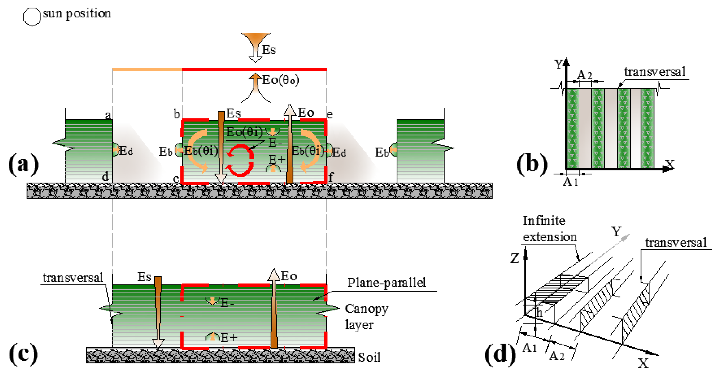
2.1. Four-Stream Radiative Transfer Equations for Continuous Crops

The four-stream radiative transfer theory was developed based on the K-M theory (it is the equations proposed by Kubelka, P. and Munk, F.; hence, it is named as K-M equations) [16,50]. The theory assumes that the canopy consists of an isolated homogeneous scattering layer (i.e., plane-parallel medium), which is composed of small and flat leaves (Figure 1c). The four-stream radiative transfer equations are written as [13]:

$$\frac{d{E}_s}{L^{\prime }dz}=k{E}_s$$

(1)

$$\frac{d{E}_{-}}{L^{\prime }dz}=-s^{\prime }{E}_s+a{E}_{-}-\sigma E_{+}$$

(2)

$$\frac{d{E}_{+}}{L^{\prime }dz}=s{E}_s+\sigma E_{-}-a{E}_{+}$$

(3)

$$\frac{d{E}_o}{L^{\prime }dz}=w{E}_s+v{E}_{-}+v^{\prime }{E}_{+}-K{E}_o$$

(4)

Here, $k$ and $K$ are extinction coefficients; $s^{\prime }$, $s$, $\sigma$, $w$, $v$, and $v^{\prime }$ are scattering coefficients; and $a$ is the attenuation coefficient. These parameters are optical coefficients in Equations (1)–(4) [19]. For unknowns in Equations (1)–(4), $E_s$, $E_{-}$, $E_{+}$, and $E_o$ are the downward specular irradiance, downward hemispherical diffuse flux density, upward hemispherical diffuse flux density, and flux-equivalent radiance in the viewing direction, respectively. Finally, $L^{\prime }$ is the differential leaf area index (also named as the leaf area density) in the vertical direction of the ccontinuous canopy, the equation for which is:

$$L^{\prime }=Lf\left({\theta }_l\right)d{\theta }_l$$

(5)

Here, $L$ is the leaf area index (LAI) and $f\left({\theta }_l\right)$ is the leaf inclination distribution function (LADF), which uses an ellipse distribution [51] (This is an equation for azimuthally independent analysis [19]).

Since $E_s$, $E_{-}$, $E_{+}$, and $E_o$ are assumed to be vertical in the four-stream radiative transfer equations (Z-axis in Figure 1d), Equation (1) describes the extinction of specular flux in the vertical direction, Equations (2) and (3) describe the vertical transfer processes of the upward and downward diffuse fluxes, and Equation (4) is an approximation of the radiative transfer equation, referring to the entire vertical radiative transfer process from the viewing [52]. Combined with the assumption that the canopy is infinitely extended (Figure 1c) for four-stream radiative transfer equations, radiative transfer of vertical flux density achieves good results in continuous crops. However, for the row canopy, there is a radiative transfer parallel to the horizontal ground surface and passing through the lateral “walls” (Figure 1a). Therefore, the lack of horizontal radiative transfer may cause an energy imbalance when crops have a row structure, which affects the accuracy of the model.

2.2. Refined Four-Stream Radiative Transfer Equations for Row-Planted Crops Considering Horizontal Radiative Transfer Equations

The radiation exchanged between the lateral “walls” and the bottom of the atmospheric boundary layer is defined as horizontal radiation, which is the diffuse radiation parallel to the horizontal ground surface and passing through the lateral “walls”. There were two lateral “walls” in the canopy closures. For one type of lateral “wall”, the emitted fluxes included specular flux and diffuse flux, which we named lateral “wall” A (“bc” Figure 1a). For the other type of lateral “wall”, the emitted flux was only the diffuse flux, which we named lateral “wall” B (“ad” and “ef” in Figure 1a). To improve the radiation energy balance issue in row-planted crops, we needed to consider this horizontal radiative transfer of the lateral “walls” into the original four-stream radiation transfer equations. According to the derivation in Supplementary Material B, we derived the horizontal radiative transfer equations, i.e., Equations (B-12), and (B-13). Combining horizontal radiative transfer equations with Equations (1)–(4), we refined the four-stream radiative transfer equation into:

$$\frac{d{E}_s}{{L^{\prime }}_{row}dz}=k{E}_s$$

(6)

$$\frac{d{E}_{-}}{{L^{\prime }}_{row}dz}=-s^{\prime }{E}_s+a{E}_{-}-\sigma E_{+}$$

(7)

$$\frac{d{E}_{+}}{{L^{\prime }}_{row}dz}=s{E}_s+\sigma E_{-}-a{E}_{+}$$

(8)

$$\frac{d{E}_o\left({\theta }_o\right)}{{L^{\prime }}_{row}dz}=w{E}_s+v{E}_{-}+v^{\prime }{E}_{+}-K{E}_o\left({\theta }_o\right)$$

(9)

$$\frac{d{E}_b}{Udz}=m^{\prime }{E}_s+g{E}_{-}+g^{\prime }{E}_{+}-n^{\prime }{E}_o\left({\theta }_i\right)$$

(10)

$$\frac{d{E}_d}{Udz}=g{E}_{-}+g^{\prime }{E}_{+}-n^{\prime }{E}_o\left({\theta }_i\right)$$

(11)

The optical coefficients (i.e., $k$, $K$, $s^{\prime }$, $s$, $\sigma$, $w$, $v$, $v^{\prime }$, and $a$) in Equations (6)–(9) used the previous equations in [19]. For the optical coefficients in the horizontal radiative transfer equations (Equations (10) and (11), the equations are:

$$n^{\prime }=1-\frac{\rho +\tau }{2}+\frac{\rho -\tau }{2}{\sin }^2{\theta }_l$$

(12)

$$g=\frac{2-\left({\sin }^2{\theta }_l-1\right)\rho -\left({\sin }^2{\theta }_l+1\right)\tau }{2\left(1+e^{-{L^{\prime }}_{row}\Delta z}\right)}$$

(13)

$$g^{\prime }=\frac{2-\left({\sin }^2{\theta }_l-1\right)\rho -\left({\sin }^2{\theta }_l+1\right)\tau }{2\left(1+e^{-{L^{\prime }}_{row}\Delta z}\right)}$$

(14)

$$m^{\prime }=\frac{A_1\left|\sin \left|{\phi }_r-{\phi }_o\right|\right|\cot {\theta }_{s}k\left(r+\tau \right)\left[2-\left({\sin }^2{\theta }_l-1\right)\rho -\left({\sin }^2{\theta }_l+1\right)\tau \right]}{4h\left(1+e^{-k{L^{\prime }}_{row}\Delta z}\right)}$$

(15)

Here, $n^{\prime }$ is the attenuation coefficient for horizontal diffuse flux, $g$ is the radiative converted coefficient describing the proportion of downward diffuse flux converted to horizontal diffuse flux from the lateral “wall”; $g^{\prime }$ is the radiative converted coefficient describing the proportion of upward diffuse flux converted to horizontal diffuse flux of the lateral “wall”; $m^{\prime }$ is the bidirectional scattering coefficient from specular flux to horizontal diffuse flux (for their derivation information see Supplementary Material B). For unknowns in Equations (10) and (11), $E_b$ is diffuse horizontal hemispheric flux density through lateral “wall” A and $E_d$ is diffuse horizontal hemispheric flux density through lateral “wall” B. Finally, ${L^{\prime }}_{row}$ is the differential leaf area index for canopy closure in the vertical direction, $U$ is the horizontal differential leaf area index, and their equations are:

$${L^{\prime }}_{row}=\left(A_1+A_2\right)Lf\left({\theta }_l\right)d{\theta }_l/A_{1}h$$

(16)

$$U=\frac{\left(A_1+A_2\right)Lf\left({\theta }_i\right)d{\theta }_i}{A_1{}^2}$$

(17)

Here, $A_1$ is the row width, $A_2$ is the distance between rows, and $h$ is the height of the canopy. According to the definition of $E_b$ and $E_d$, $E_b$ and $E_d$ are horizontal radiation in lateral “wall” A and lateral “wall” B, respectively. Therefore, Equation (10) is the horizontal radiative transfer equation in lateral “wall” A and Equation (11) is the horizontal radiative transfer equation in lateral “wall” B. These two equations are considered, and the entire system of equations satisfies the radiation energy balance for the canopy closure of row-planted crops.

We used z = 0 and z = −1 as the boundary conditions in the vertical direction, and $B=\frac{A_1}{2h}\left|\sin \left|{\phi }_r-{\phi }_o\right|\right|$ (it’s acquired in Supplementary Material B-2) as the boundary conditions in the horizontal direction to solve Equations (6)–(11). We calculated the directional reflectance factor (DRF) on the boundary of the canopy closure; that is, the DRF at the top of the canopy closure ($R_c$) and the DRFs of lateral “wall” A ($R_b$) and lateral “wall” B ($R_d$). Among them, for the DRF at the top of canopy closure ($R_c$), we referred to the solution in the original four-stream radiative transfer equations (i.e., Equations (29)–(33) in Section 2.3.1). For the DRFs of lateral “wall” A ($R_d$) and lateral “wall” B ($R_d$), we showed the derivation in Supplementary Material D. The equation for the DRF of lateral “wall” A is:

$$R_b=\frac{r_{\parallel }{}_{s\overline{d}}{E}_{\parallel s}\left(B\right)+r_{\parallel }{}_{\overline{d}o}{E}_{\parallel \pm }\left(B\right)}{E_{\parallel s}\left(B\right)+E_{\parallel \pm }\left(B\right)}$$

(18)

and the equation for the DRF of lateral “wall” B is:

$$R_d=\frac{r_{\parallel }{}_{so}{E}_{\parallel s}\left(B\right)+r_{\parallel }{}_{d\overline{d}}{E}_{\parallel \pm }\left(B\right)}{E_{\parallel s}\left(B\right)+E_{\parallel \pm }\left(B\right)}$$

(19)

Here, $E_{\parallel s}\left(B\right)$ is the specular flux on the surface of the lateral “wall” and $E_{\parallel \pm }\left(B\right)$ is the diffuse flux on the surface of the lateral “wall”. Their equations are:

$$E_{\parallel s}\left(B\right)={\rho }_{s\overline{d}}{E}_s(0)$$

(20)

$$E_{\parallel \pm }\left(B\right)={\rho }_{d\overline{d}}{E}_{-}\left(0\right)+{{\rho }^{\prime }}_{d\overline{d}}\left\{\left[e^{-L_{row}}{E}_{-}\left(0\right)+e^{-k{L}_{row}}{E}_s\left(0\right)\right]r_s\right\}$$

(21)

Here, $r_{\parallel }{}_{s\overline{d}}$, $r_{\parallel }{}_{\overline{d}o}$, $r_{\parallel }{}_{so}$, and $r_{\parallel }{}_{d\overline{d}}$ in Equations (18) and (19) are:

$$r_{\parallel }{}_{s\overline{d}}=\frac{o_1{o}_2{{\rho }^{\prime }}_{d\overline{d}}\left(D_1+{\tau }_{dd}{\rho }_{s\overline{d}}{\tau }_{oo}\right)}{o_3\left(M_1+o_1{\tau }_{dd}{\rho }_{s\overline{d}}{\tau }_{oo}\right)}$$

(22)

$$r_{\parallel }{}_{d\overline{d}}=\frac{o_1{o}_2{\rho }_{\overline{dd}}\left(D_1+{\tau }_{dd}{\rho }_{s\overline{d}}{\tau }_{oo}\right)}{o_3{M}_2}$$

(23)

$$r_{\parallel }{}_{so}=\frac{o_1{o}_2{{\rho }^{\prime }}_{d\overline{d}}{D}_1}{o_3{M}_1}$$

(24)

$$r_{\parallel }{}_{\overline{d}o}=\frac{o_1{o}_2{\rho }_{\overline{dd}}{D}_1}{o_3{M}_2}$$

(25)

With the calculated results of these DRFs, we then combined the area fractions of each component in row crops calculated from the gap probabilities (Supplementary material C) and DRF at the top of between row area ($R_{br}$) (it was calculated from the integral radiative transfer equation in Supplementary material E) to build a row-planted crop model to calculate the DRF.

2.3. Sum of the Directional Reflectance Factor of Row-Planted Crops

We followed the assumption that the canopy extended infinitely in the four-stream radiative transfer equations [19], and the row canopy also alternated between canopy closure and between row to reach infinite extension. Therefore, the DRF at the top of canopy closure ($R_c$) and the DRF at the top of the between row area ($R_{br}$) composed the sum DRF of row-planted crops, namely:

$$R_{sum}=\frac{1}{A_1+A_2}\left(A_1{R}_c+A_2{R}_{br}\right)$$

(26)

According to the composition of the DRFs in Equation (26), we explained the calculation for DRF at the top of the canopy closure and at the top of the between row area, respectively.

2.3.1. Directional Reflectance Factor of the Canopy Closure

In the field of radiative transfer, the DRF at the top of the canopy closure included the single scattering ($R_{c\_1}$) and the multiple scattering of the canopy closure ($R_{c\_m}$), the equation for which is:

$$R_c=R_{c\_1}+R_{c\_m}$$

(27)

Below is the DRF derived from the original four-stream radiative transfer equations in [13]:

$$R=\frac{r_{so}^{*}{E}_s\left(0\right)+r_{do}^{*}{E}_{-}\left(0\right)}{E_s\left(0\right)+E_{-}\left(0\right)}$$

(28)

This equation shows that the DRF includes the bidirectional reflectance factor ($r_{so}^{*}$) and the hemispherical directional reflectance factor ($r_{do}^{*}$), which is the ratio of the reflected flux ($r_{so}^{*}{E}_s\left(0\right)+r_{do}^{*}{E}_{-}\left(0\right)$) to the incident flux ($E_s\left(0\right)+E_{-}\left(0\right)$) at the top of the canopy. The canopy closures are different from the continuous canopy—they are separated by between rows (Figure 1a). In this section, the differential leaf area index (leaf area density) (${L^{\prime }}_{row}$) and the area fractions of each component ($S$) changed according to the row structure. Therefore, to solve the canopy closure using the solution method in the original four-stream radiative transfer theory, ${L^{\prime }}_{row}$ and $S$ needed to be modified according to the structure. The differential leaf area index (leaf area density) for canopy closure in the vertical direction was modified in Equation (16), and the area fractions of each component were modified in Table C-1 in Supplementary Material C. With these modifications, the solution for the original four-stream radiative transfer equations could be used to calculate the single scattering of the canopy closure and the multiple scattering of the canopy closure.

Single Scattering of the Canopy Closure

According to [13], we used the following equation to calculate the single scattering of the canopy closure ($R_{c\_1}$):

$$R_{c\_1}=\frac{r_{so\_\mathrm{c}\_1}^{*}{E}_s\left(0\right)}{E_s\left(0\right)+E_{-}\left(0\right)}$$

(29)

in which:

$$\begin{array}{l}{r}_{so\_c\_1}^{*}=r_{so\_v}^1+r_{so\_s}^1\\ =w{L^{\prime }}_{row}{S}_{closure\_s}(z)+S_{closure\_s}(h)r_s\end{array}$$

(30)

Here, $r_{so\_v}^1$ is the single scattering of specular flux in the canopy closure, $r_{so\_s}^1$ is the single scattering of specular flux from the soil in the canopy closure, and $r_s$ is the DRF of the soil. $S_{closure\_s}(z)$ is the fraction of observed canopy illuminated by the specular flux in the canopy closure, $S_{closure\_s}(h)$ is the fraction of observed soil illuminated by the specular flux in the canopy closure, and their expressions are shown in Table C-1 in Supplementary Material C.

Multiple Scattering of the Canopy Closure

According to [13], we used the following equation to calculate the multiple scattering of the canopy closure:

$$R_{c\_m}=\frac{r_{so\_c\_m}^{*}{E}_s\left(0\right)+r_{do\_c}^{*}{E}_{-}\left(0\right)}{E_s\left(0\right)+E_{-}\left(0\right)}$$

(31)

in which:

$$\begin{array}{l}{r}_{so\_c\_m}^{*}=r_{so\_v}^m+r_{so\_s}^m\\ =S_{closure\_d}\left[\begin{array}{l}\frac{\left(v+v^{\prime }{r}_{\infty }\right)T_1+\left(r_{\infty }v+v^{\prime }\right)T_2}{1-r_{\infty }^2}\\ -\left(\begin{array}{cc}{Q}_v& P_v\end{array}\right){\left[\begin{array}{cc}1& r_{\infty }{e}^{-m{L^{\prime }}_{row}{\Omega }_E}\\ r_{\infty }{e}^{-m{L^{\prime }}_{row}{\Omega }_E}& 1\end{array}\right]}^{-1}\left(\begin{array}{c}{Q}_s\\ P_s\end{array}\right)r_{\infty }/1-r_{\infty }^2\end{array}\right]\\ +\left(S_{closure\_d}{r}_s\right)\left\{\left[\left({\tau }_{ss}+{\tau }_{sd}\right){\tau }_{do}+\left({\tau }_{sd}+{\tau }_{ss}{r}_s{r}_{dd}\right){\tau }_{oo}\right]\frac{1}{1-r_s{r}_{dd}}\right\}\end{array}$$

(32)

$$\begin{array}{l}{r}_{do\_c}^{*}=r_{do}^1+r_{do}^m\\ =S_{closure\_d}\left\{r_{do}+\left[({\tau }_{do}+{\tau }_{oo}){\tau }_{dd}\frac{1}{1-r_s{r}_{dd}}\right]r_s\right\}\end{array}$$

(33)

Here, $r_{so\_v}^m$ is the multiple scattering of specular flux in the canopy closure, $r_{so\_s}^m$ is the multiple scattering of specular flux between soil and vegetation in the canopy closure, $r_{do}^1$ is the single scattering of diffuse flux in the canopy closure, and $r_{do}^m$ is the multiple scattering of diffuse flux in the canopy closure. $S_{closure\_d}$ is the fraction of canopy closure illuminated by the diffuse flux, and its expressions are shown in Table C-1 in Supplementary Material C.

2.3.2. Directional Reflectance Factor of the Between Row Area

Similar to Section 2.3.1, the DRF at the top of the between row area included the single scattering of the between row area ($R_{br\_1}$) and the multiple scattering of the between row area ($R_{br\_m}$), the equation for which is:

$$R_{br}=R_{br\_1}+R_{br\_m}$$

(34)

Single Scattering of the Between Row Area

The single scattering of the between row area is:

$$R_{br\_1}=\frac{r_{so\_br\_1}^{*}{E}_s\left(0\right)}{E_s\left(0\right)+E_{-}\left(0\right)}$$

(35)

in which:

$$r_{so\_br\_1}^{*}=S_{between\_row\_s}{r}_s$$

(36)

Here, $S_{between\_row\_s}$ is the fraction of observed soil background in the between row area illuminated by the specular flux, and its expressions are shown in Table C-1 in Supplementary Material C.

Multiple Scattering of the Between Row Area

The multiple scattering of the between row area is:

$$R_{br\_m}=S_{between\_row\_d}{R}_{s\_m}$$

(37)

Here, $R_{s\_m}$ is the multiple-scattering of soil in the between row area, which is:

$$R_{s\_m}=\frac{a_s{k}_{B\left(A\right)\to C}\left(R_b+R_d\right)+2a_s{n}^{\prime }{k}_{B\left(A\right)\to C}{k}_{C\to A\left(B\right)}{R}_s}{1-k_{B\left(A\right)\to A\left(B\right)}-2a_s{n}^{\prime }{k}_{B\left(A\right)\to C}{k}_{C\to A\left(B\right)}}$$

(38)

We calculated this parameter based on the solution for the integral form radiative transfer equation. For detailed calculation, please refer to Supplementary Material E. $S_{between\_row\_d}$ is the fraction of the between row background illuminated by the diffuse flux. Its expressions are shown in Table C-1 in Supplementary Material C. We used the horizontal DRFs (i.e., $R_b$ and $R_d$) as the initial values to calculate the multiple scattering of the between row area.

2.4. Input Parameters of the MFS Model

Based on the above mathematical analysis, we refined the four-stream radiative transfer equations by considering the horizontal radiative transfer equations, and then solved them to build the model for row-planted crops combined with the reflectance issue of the between row reflectance, then proposed the MFS model. In the MFS model, the directional hemisphere reflectance and transmittance of leaves are provided by the PROSPECT-5 simulations [53,54]. The input parameters of MFS include:

(1)

Geometrical parameters: solar zenith angle (${\theta }_s$), solar azimuth angle (${\phi }_s$), viewing zenith angle (${\theta }_o$), viewing azimuth angle (${\phi }_o$), and row azimuth angle (${\phi }_r$);

(2)

Canopy parameters: height of the canopy ($h$), row width ($A_1$), distance between rows ($A_2$), leaf area index ($L$) and effective leaf area index ($L_E$), average leaf inclined angle (${\theta }_l$), and canopy dimension parameter ($l_L^{*}$);

(3)

Biochemical leaf parameters: chlorophyll content ($C_{ab}$), carotenoid content ($C_{ar}$), brown pigment content ($C_{brown}$), equivalent water thickness ($C_w$), leaf mass per unit leaf area ($C_m$), and structure coefficient ($N$);

(4)

Canopy radiative parameters: the fraction of incoming diffuse radiation ($skyl$).

3. Data

In this study, we validated the MFS model using both computer simulation and in situ measurements.

3.1. Computer-Simulated Data

In the study of the canopy radiative transfer model, the simulation of the canopy radiative transfer assumed that there was no influence from the atmosphere. Since the in situ measurement is done in the atmospheric environment, it is difficult to exclude the influence of essential climate variables (ECVs) on the “true value” of the measurement [55]. According to the radiation transfer model intercomparison (RAMI), the DRF calculated by 3D computer simulation has the highest accuracy, and the calculation result can be used as a “surrogate truth” to validate the turbid medium model in radiative transfer [56,57,58]. The MFS model in this study is based on the radiative transfer equations of flux density in order to calculate the reflectance. Therefore, we used a 3D computer simulation based on the principle of flux density to validate the MFS model. The 3D computer simulation is the extended a 3D radiosity graphics (RGM) model [11,59]. The RGM model is a radiosity model based on a bilinear equation (a simple non-linear differential equation) [5]. It uses numerical calculation methods to calculate the scattering of polygons in a scene constructed by a computer graphics method and has high calculation accuracy [11]. To use the RGM model to validate the MFS model, we first needed to use computer graphics to construct the abstract scenes that were assumed to have medium turbidity, and then set the inputs and outputs for the two models.

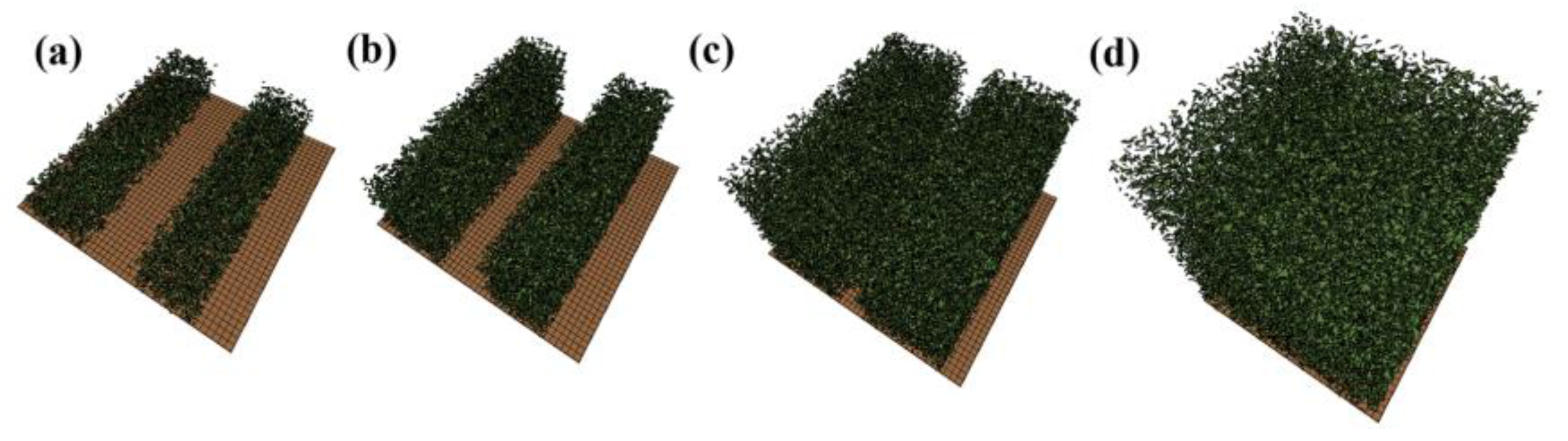
3.1.1. Generation of Computer Abstract Scenes

According to the study in the fourth phase of the radiative transfermodel intercomparison (RAMI-IV, http://rami-benchmark.jrc.ec.europa.eu), the establishment of the scene is based on measurements [60]. Therefore, measurements of corn during the growth period in the Yingke Oasis (see Section 3.2.1 for details) were used to establish the abstract scenes [61]. The abstract scene was generated (Figure 2), in which the canopies with four geometric structures were generated to reflect the row growth state, including the proportion of between row dominance (stage_rv1), proportions of between row and canopy closure equality (stage_rv2), the proportion of canopy closure dominance (stage_rv3), and continuous vegetation (stage_cv). The parameters of the constructed abstract scene are listed in

Table 1. Values of parameters in the constructed abstract scene.

Scene1	Figure 2	A1 (m)	A2 (m)	h (m)	L (m•m−1)	n△ (-)	w*△ (m)	l*△ (m)	θl (°)	φr (°)
Stage_rv1	(a)	0.4	0.6	0.48	0.58	10,419	0.02	0.02	44	0
Stage_rv2	(b)	0.5	0.5	0.88	1.75	25,840	0.02	0.02	44	0
Stage_rv3	(c)	0.75	0.25	1.28	3.51	48,325	0.02	0.02	44	0
Stage_cv	(d)	1	0	1.58	5.11	40,262	0.02	0.02	44	0

Here, the shape of the leaf is triangular, with the area ranging from 0.0002 m² to 00003m² in the scenes; the shape of the soil area is square, with an area of 0.0025 m²; and the leaf inclined angle is randomly distributed in the zenith and azimuth directions. The symbols in Table 1 are: A₁ = row width, A₂ = distance of between-rows, h = the height of the canopy, L = leaf area index, n_△ = the number of triangular leaves, w*_△ = one of the short sides of the horizontal triangle leaf, l*_△ = the other short sides of the horizontal triangle leaf, θ_l is average leaf inclined angle. φ_r is row azimuth angle.

.

3.1.2. Input and Output Settings for Computer-Simulated Validation

Input Setting

In both the RGM model and MFS model, the directional hemisphere reflectance and transmittance of leaves were provided by the PROSPECT-5 model. The input parameters of PROSPECT-5 model (C_ab = 40.29 ug·cm⁻², C_ar = 8.54 ug·cm⁻², C_brown = 0, N = 1.52, Cw = 0.014 cm⁻², C_m = 0.004 g·cm⁻²) were also obtained (see Section 3.2.1 for details). The soil reflectance was obtained by measurement, in which the red band with 670 nm was 0.242 and the near-infrared band with 850 nm was 0.314. According to data from the Yingke Oasis, the sun zenith angle was 25° and the sun azimuth angle was 130°. To keep the flux density in both the MFS model and RGM model consistent, we changed the measured flux density to the normalized flux density in the validation. In the MFS model, this took into account the diffuse incidence (Equation (33)) at the top of the canopy that was ignored by the previous row model [40], for which the fraction of incoming diffuse radiation ($skyl$) for both models was set to 0.1. Combined with Equation (C-22) in Supplementary Material C, $n_{\Delta }$, $l_{*△}$, and $w_{*△}$ in Table 1 were used to calculate the canopy dimension parameter ($l_L^{*}$) in the MFS model. Finally, for the row structure and in the MFS model, we used the measured values of the Yingke Oasis (i.e., the values of the abstract scene in Table 1).

Output Setting

Previous studies showed that there was a systematic error in the four-stream radiative transfer equations when the viewing azimuth angle was greater than 40°, and this phenomenon was particularly obvious in the NIR band [40]. To better show that the MFS model had solved this problem, we showed the DRF field of the entire hemisphere space—simulations were performed with the viewing azimuth angle varying from 0 to 350° with a step of 10°, and with the viewing zenith angle ranging from 0 to 89° with a step of 5°. One thing needs to be explained—the MFS model assumed that the canopy was an infinite extension. To unify the comparison conditions, we chose the infinite canopy mode in RGM to calculate the DRF. The infinite canopy does not just calculate the DRF of the finite canopy for the 1- to 2-row cycle shown in Figure 2, but copies the finite canopy for $101\times 101$ times as a duplicated canopy to obtain an approximately infinite extension, and then calculates the DRF of this infinite canopy (shown in Appendix B in [11]) as its calculation principle. When the viewing zenith angle was 90°, the RGM model was unable to be simulated. Therefore, the maximum angle is 89°. Finally, Figures 3, 5, 7, and 9 show the DRF fields simulated by both models, while Figures 4, 6, 8, and 10 show the corresponding four viewing modes for row-planted crops in DRF fields, i.e., the principal plane (PP, viewing azimuth angle is aligned with solar azimuth angle), orthogonal plane (OP, viewing azimuth angle is perpendicular to solar azimuth angle), along row plane (AR, the plane is along the row direction), and orthogonal row plane (OR, the plane is perpendicular to the row direction).

3.2. In Situ Data

3.2.1. Measurement Experiment

The in situ data were collected in the Watershed Allied Telemetry Experiment Research (WATER) project, ranging from May 20 to July 9, 2008, in the site located at 38.8571°N, 100.4104°E, at an elevation of 1529 m [62,63]. This is a cornfield located in the Yingke Oasis, Zhangye City, Gansu Province, China. The area of the plots is 180 × 180 m. In each plot, three samples were randomly selected to perform measurements [64]. The measurements included two of the crop canopy, one of row-planted crops at the jointing stage, and the other of continuous crops at the heading stage. The data used in this study were introduced as outlined below.

Directional Reflectance Factor (DRF)

The DRF of the corn and the DRF of soil at wavelengths ranging between 400 and 2500 nm were measured using the Spectrometer (It name is ASD FieldSpec Pro Spectrometer) mounted on a multi-angle observation frame. The distance from the sensor to the bottom of the canopy was 5 m, and the viewing angle under FOV was 25° during the measurement. The viewing azimuth angle varied from 0° to 360° along the azimuth of the plane (i.e., four viewing modes described below), while the zenith angle varied from −60° (i.e., backward direction) to 60° (i.e., forward direction) with an interval of 10°. For further analysis of the anisotropy of DRFs for row-planted crops, these measurements were separated into four categories according to four viewing modes, namely PP, OP, AR, and OR.

Canopy Structural and Leaf Biochemical Parameters

The effective leaf area index and average leaf angle were measured using the LAI-2000. The leaf area index, row width, distance between rows, average canopy height, row azimuth angle, average width of leaves, average length of leaves, and average area of leaves were simultaneously measured using the direct measuring method (the leaf area index was measured using the improved harvesting method—IHM [65]) [61]. The chlorophyll content was calculated using the empirical formula based on the SPAD index (this is a vegetation index that determines the chlorophyll in the leaf), acquired using the SPAD chlorophyll meter [66,67]. The leaf mass per unit leaf area ($C_m$) and the equivalent water thickness ($C_w$) were derived from the weights of fresh and dry leaves [68], given in g·cm⁻² [69]. The carotenoid content ($C_{ar}$), brown pigment content ($C_{brown}$), and structure coefficient ($N$) were determined using the Lopex1993 database [70].

3.2.2. Input and Output Settings for In Situ Validation

Input Setting

In the DRM, SAIL, and MFS models, the directional hemisphere reflectance and transmittance of leaves are provided by the PROSPECT-5 model. The input parameters of the PROSPECT-5 model are Cab = 40.29 ug·cm⁻², Car = 11.41 ug·cm⁻², Cbrown = 0, N = 1.52, Cw = 0.014 cm⁻², and Cm = 0.004 g·cm⁻². To keep the leaf inclination distribution function (LADF) in the comparison consistent, we replaced the LADF of the ellipse distribution in the SAIL model and the MFS model with the LADF based on the graphic method [52], as in the DRM model. Considering that the DRM model does not consider the clumping index issue, we divided the MFS model into two types: one version where the clumping index was considered (MFS₁), and one version where the clumping index was not considered (MFS₂). In MFS₁, the canopy dimension parameter ($l_L^{*}$) used the equation proposed in the DRM model, (i.e., Equation (C-9) in Supplementary Material C). In MFS₂, the canopy dimension parameter ($l_L^{*}$) used Equation (C-18) in Supplementary Material C. Finally,

Table 2. Values of input parameters in the MFS, DRM, and SAIL models for simulation of the DRFs of corn.

Vegetation Type	Model	L (m•m−1)	LE (m•m−1)	LIDFa	LIDFb	A1 (m)	A2 (m)	h (m)	skyl (-)	θo (°)
RC	MFS1	2.51	2.51	0.38	−0.02	0.46	0.46	0.98	0.1	60
	MFS2	2.51	1.73	0.38	−0.02	0.46	0.46	0.98	0.1	60
	DRM	2.51	-	0.38	−0.02	0.46	0.46	0.98	0.1	60
CC	MFS	3.99	3.99	0.38	−0.02	1	0	1.54	0.1	0
	SAIL	3.99	-	0.38	−0.02	-	-	-	0.1	0

Here, the abbreviations in the title are: MFS = modified four-stream radiative transfer model; DRM = a spectral directional reflectance model; SAIL = light scattering by leaf layers with application to canopy reflectance modeling. The symbols in Table 2 are: L = leaf area index, L_E = effect leaf area index, A₁ = row width, A₂ = distance of between-rows, h = the height of the canopy, skyl = fraction of incoming diffuse radiation, and θ_o = viewing zenith angle, RC = row-planted crops and CC = continuous crops. LIDFa and LIDFb are the controlling parameters from the graphical method, which controls leaf inclination angle distribution function. LIDFa and LIDFb are obtained from the average leaf inclinated angle and the variance of the leaf inclinated angle in the measurement, and their equation are found in [71].

showed other input parameters in the three models.

Output Setting

To validate whether the MFS model improves the accuracy of canopy reflectance of row-planted crops at zenith angles greater than 40°, we chose ${\theta }_o=\pm 60°$ and ${\theta }_o=\pm 50°$ as quasi-horizontal DRFs to be used in the validation. On this basis, to further reflect the reflectance anisotropy issue, we selected three measurement modes that lateral “walls” may observe, namely PP, OP, and OR. To further show that the MFS model had improved the accuracy of the canopy reflectance when the viewing azimuth angle was greater than 40° compared with the previous model, we chose the original row model for comparison, i.e., the DRM model [40]. To further assess the applicability of the model for the continuous crops, simulations of the SAIL model were also used for comparison with the simulations of the MFS model in the vertical viewing direction (${\theta }_o=0°$). Finally, Figures 11 and 12 show the corresponding DRF simulations and in situ measurements.

4. Results

4.1. Validation of MFS Model Using Computer-Simulated Data

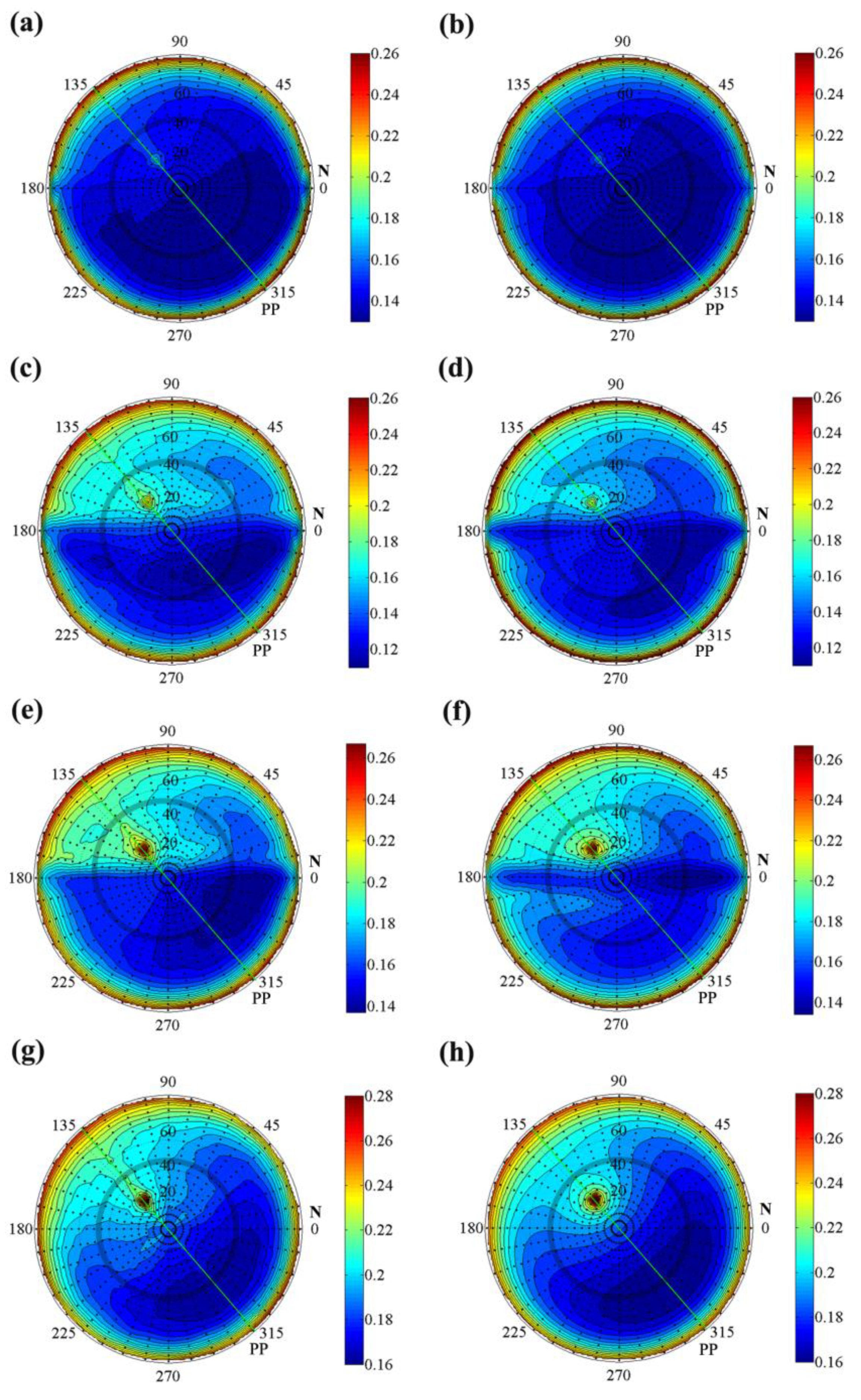
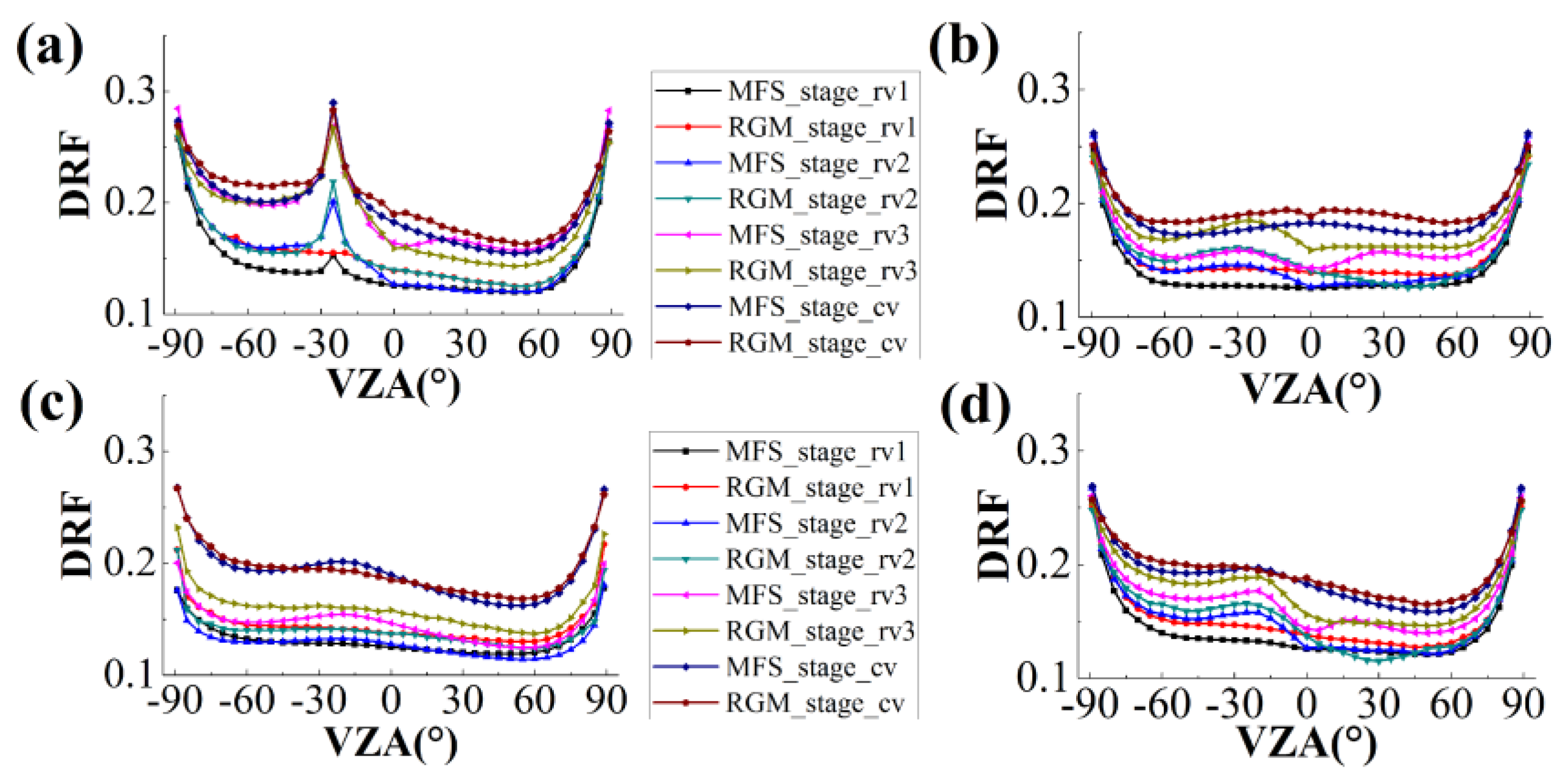
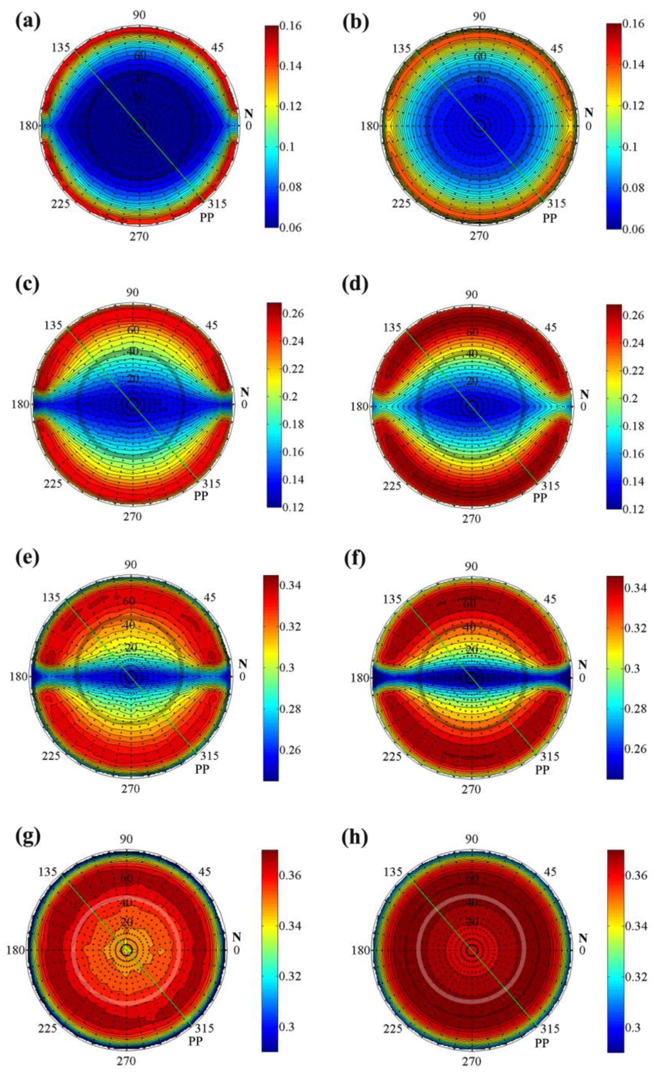
4.1.1. Results of the Qualitative Analysis of DRFs in the Red Band

In Figure 3, the RGM model and MFS model were used to simulate the DRF fields in red band (670 nm) changes in the growing stage of the crops, including DRFs for three stages for row-planted crops and DRFs for one stage for continuous crops. The figure results show that the values of DRF fields simulated by the MFS model are highly consistent with the values of DRF fields simulated by the RGM model, especially in the DRF fields with zenith angles greater than 40° (outside of shaded annulus in Figure 3). The contours of the fields are slightly different. However, the magnitude of the DRF fields simulated by the two models is between 10⁻³ and 10⁻², and the difference between the two model simulations is not more than 16.69% (

Table 3. Statistics for comparison of the DRFs simulated by the MFS model versus DRFs derived from the RGM model for four scenes.

Scenes.	Statistics	DRF_red	DRF_NIR	DRF_NIR_1	DRF_NIR_m
Stage_rv1	R	0.9842	0.9900	0.9881	0.9846
	RMSE	0.0018	0.0082	0.0038	0.0063
	Average difference	−16.69%	−7.49%	9.41%	−22.64%
Stage_rv2	R	0.9788	0.9807	0.9667	0.9864
	RMSE	0.0017	0.0141	0.0087	0.0079
	Average difference	−13.76%	−11.69%	−9.99%	3.35%
Stage_rv3	R	0.9341	0.9352	0.9714	0.9610
	RMSE	0.0008	0.0186	0.0065	0.0112
	Average difference	4.80%	−0.48%	−1.02%	−0.10%
Stage_cv	R	0.9662	0.8207	0.9895	0.9084
	RMSE	0.0005	0.0083	0.0035	0.008
	Average difference	−5.25%	1.53%	1.16%	−3.02%

Here DRF_red = DRF in red band, DRF_NIR=DRF in NIR band, DRF_NIR_1 = singlescattering of DRF in NIR band, DRF_NIR_m = multiple scattering of DRF in NIR band, Stage_rv1 = the proportion of between row dominance, Stage_rv2 = proportions of between row and canopy closure equality, Stage_rv3 = the proportion of canopy closure dominance, and Stage_cv = continuous vegetation, R = correlation coefficient, RMSE = root mean squared error, Average difference is ${\displaystyle \sum _i\left[\left(A-B\right)/A\right]\times 100\%}$; here, A denotes the DRF of the RGM model, B denotes the DRF of the MFS model, and i is the number of interpolation points in the DRF field. The negative numbers represent an overestimation and the positive numbers represent an underestimation.

). Hence, the difference is very small. From Figure 5a,b to Figure 5g,h, the high-value area generated by the soil background shrinks into hotspots as the crop grows. In the cross-sectional view of the DRF fields, i.e., Figure 4, the difference in the contours of the fields in Figure 3 is very small. For the four viewing modes in the red band, DRFs simulated by the MFS model and DRFs simulated by the RGM model are more consistent, except for the simulation at a viewing zenith angle greater than 80° along row plane (AR) mode (Figure 4c).

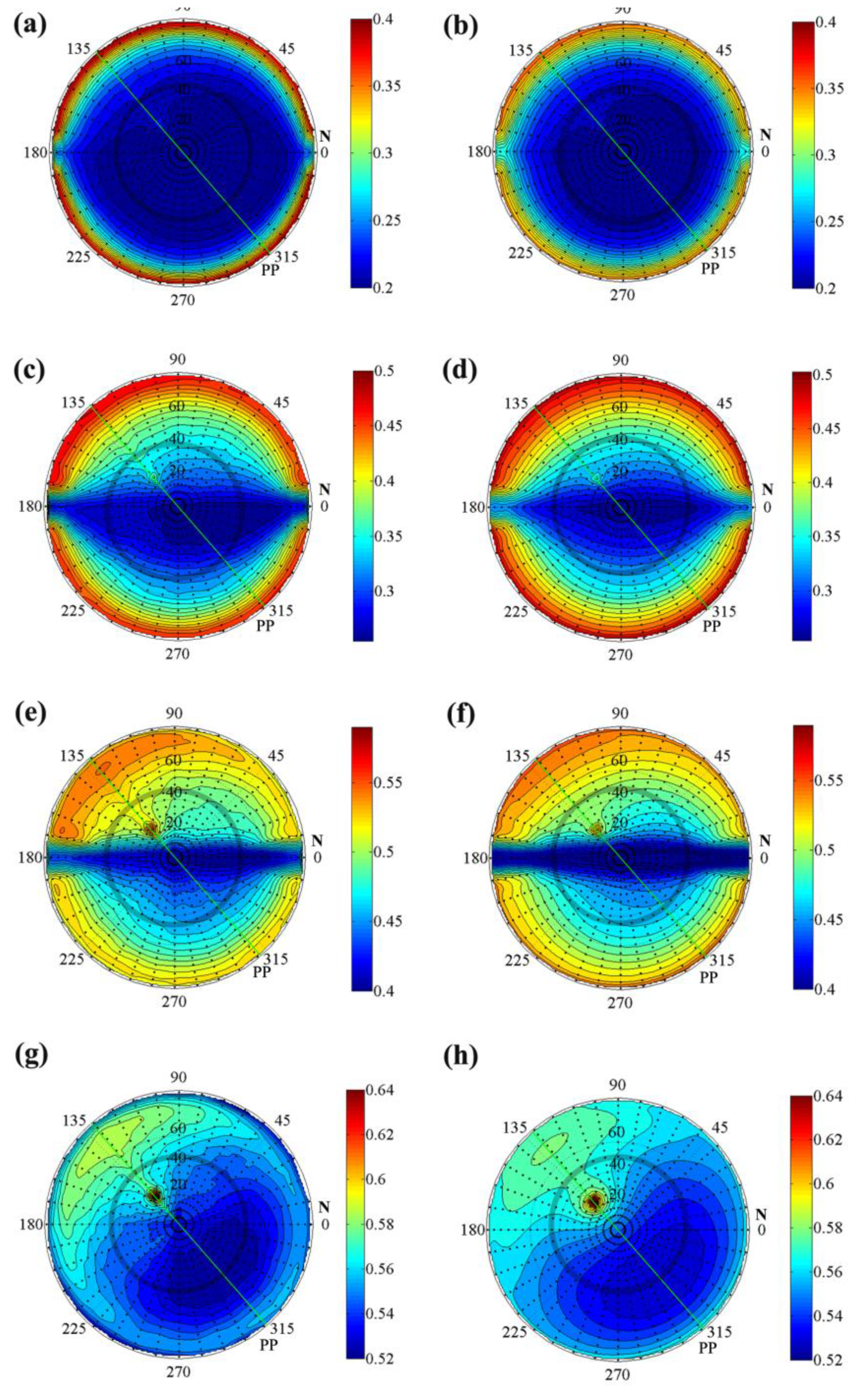
4.1.2. Results of the Qualitative Analysis of DRFs in the NIR Band

Figure 5 shows the DRF fields of the growth stages of crops in the NIR band (850 nm) simulated by the RGM model and the MFS model. The DRFs simulated by the MFS model and the DRF simulated by the RGM model are very consistent at zenith angles greater than 40° (outside of shaded annulus in Figure 5), and the difference between the two models does not exceed 11.69% (Table 3). Different from the shape of DRF fields in the red band, the shape of DRF fields in the NIR band presents a bowl-shape (Figure 5). In the growth stage of the DRF fields, the bowl edges (the area where the reflectance increases rapidly) shrink toward a small zenith angle, e.g., the bowl edge is around 80° for stage_rv1 (Figure 5a,b), around 70° for stage_rv2 (Figure 5c,d), around 60° for stage_rv3 (Figure 5e,f). From the AR direction, i.e., stripe area from 0 to 180 ° in the DRF fields, there is a distinct low-value area. Among the cross-sectional views of the four viewing modes in Figure 5, namely Figure 6, the DRFs simulated by the MFS model and the DRFs simulated by the RGM model have higher consistency.

Unlike the red band, the multiple scattering effects of the NIR band can be ignored. For the NIR band, it is very important. To further analyze the differences between the RGM model and the MFS model in the simulations, DRFs in the NIR band are divided into two groups, i.e., single scattering and multiple scattering DRFs. For single scattering, the difference between the two models does not exceed 9.99% (Table 3). When the zenith angle is greater than 40° (outside of shaded annulus in Figure 7), the consistency between the DRFs simulated by the two models is very high (Figure 7). When the row structure is obvious (Figure 7c–f), the low-value area for the DRFs appears in the opposite direction to the incident hemisphere (${\phi }_o\in \left[{180}^{\circ },{360}^{\circ }\right]$). The high-value area due to the hotspot effect appears in the second quadrant of the polar coordinates systems (${\phi }_o\in \left[{90}^{\circ },{180}^{\circ }\right]$), and a curved low-value area appears in the first quadrant (${\phi }_o\in \left[0^{\circ },{90}^{\circ }\right]$). For the DRF fields in Figure 7b,d,f,h, the lowest DRF values are in the fourth quadrant of the polar coordinates (${\phi }_o\in \left[{270}^{\circ },{360}^{\circ }\right]$). Figure 8 shows the single scattering of DRF in the four viewing modes in the NIR band. Although the values for LAI = 0.58 in Figure 8a were slightly different, the overall consistency was high.

Figure 9 displays changes in the growing stage of the crops due to the multiple scattering of the NIR band. This shows that the DRFs simulated by the MFS model are slightly higher than DRFs simulated by the RGM model, and the difference between the two models does not exceed 3.35%, except for stage_rv1 (Figure 9a,b). With changes in the row structure, the low-value area shrinks toward the center of the row angle. For the cross-sections of the four viewing modes in Figure 10, the DRFs of the multiple scattering simulated by the MFS model are highly consistent with the DRFs of the multiple scattering simulated by the RGM model.

4.1.3. Quantitative Analysis Results

The results of the qualitative analysis between the two models are shown in Section 4.1.1 and Section 4.1.2. To further describe the comparison between the two models, we present the results of the quantitative analysis. Figure 3, Figure 5, Figure 7 and Figure 9 include 684 samples simulated under the same sun and viewing geometries for each abstract scene. The average difference of the DRF fields between the two models is summarized in Table 3. In Table 3, the average difference between the DRF simulated by the MFS model and the DRF simulated by the RGM model is generally not more than 10%, except for DRF in red band (DRF_red) (−16.69%) and multiple scattering of DRF in NIR band (DRF_NIR_m) (−22.64%) in the stage_rv1. On the same computer with the same configuration, the calculation time for the MFS model was 0.135 hours for all of the scenes, while the calculation time for the RGM model was 5.678 hours for all of the scenes. In Table 3, the DRFs simulated by the MFS model show good correlation with DRFs simulated by the RGM model, with correlation coefficients greater than 0.9341, except for the DRFs in the NIR band in stage_cv (R = 0.8207). RMSEs are less than 0.0019 in the red band and less than 0.0187 in the NIR band. The MFS model simulates the DRFs contributed by single scattering and multiple scattering in the NIR band with good accuracy, i.e., R is greater than 0.96 and RMSEs are less than 0.0088 for single scattering, while R is greater than 0.9 and RMSEs are less than 0.012 for multiple scattering.

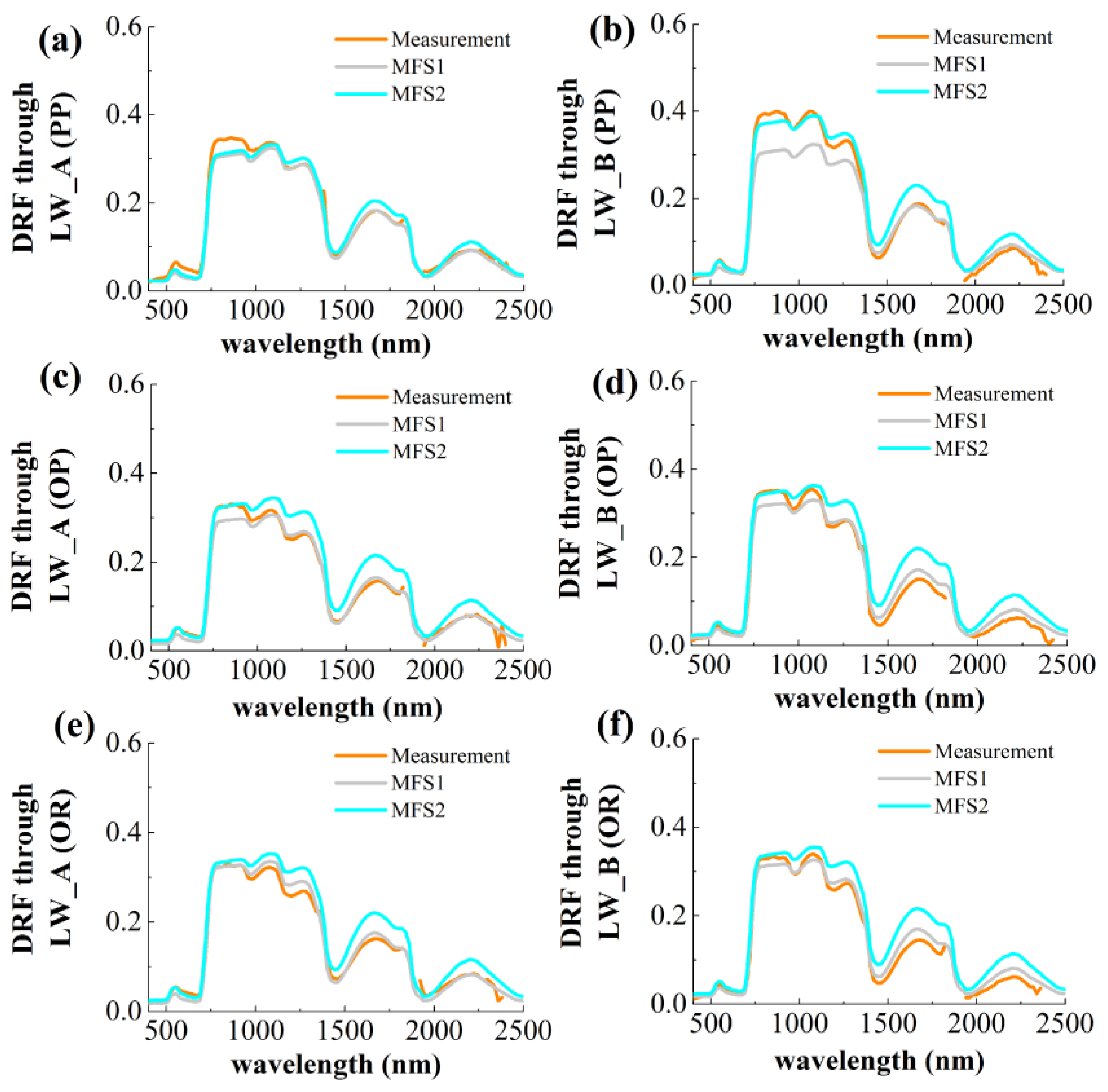
4.2. Validation of the MFS Model Using In Situ Data

Figure 11a–f and Figure 12a–f show the simulation differences between the row models under the PP, OR, and OP at zenith angles of 60° and 50°, respectively. MFS₁ and MFS₂ are highly consistent with the measured data. The DRFs simulated by MFS₂ are better than the DRFs simulated by MFS₁, and their correlation coefficients (R) are higher than 0.985 with RMSEs of less than 0.023 (

Table 4. Summary of statistics for the comparison of the simulated DRFs versus in situ measurements.

	RC(PP)				RC(OP)				RC(OR)				CV
	lateral wall A		lateral wall B		lateral wall A		lateral wall B		lateral wall A		lateral wall B
	R	RMSE	R	RMSE	R	RMSE	R	RMSE	R	RMSE	R	RMSE		R	RMSE
DRM	0.997	0.012	0.997	0.011	0.990	0.026	0.998	0.010	0.996	0.017	0.999	0.008	SAIL	0.998	0.012
MFS1 (60)	0.994	0.013	0.997	0.008	0.989	0.020	0.998	0.009	0.996	0.017	0.998	0.006	MFS	0.998	0.012
MFS2 (60)	0.996	0.010	0.998	0.007	0.990	0.018	0.999	0.006	0.996	0.011	0.998	0.006
MFS1 (50)	0.991	0.016	0.994	0.012	0.996	0.012	0.995	0.013	0.996	0.011	0.996	0.011
MFS2 (50)	0.991	0.018	0.990	0.016	0.990	0.019	0.986	0.022	0.991	0.018	0.987	0.021

Here RC = row-planted crops, CC = continuous crops, PP = principal plane, OP = orthogonal plane, OR = orthogonal row.

). The DRF simulated by the DRM model is seriously overestimated when the zenith angle is greater than 40°, especially in the NIR band (Figure 11a–f). Comparatively, the DRF simulated by MFS₁ and MFS₂ at the zenith angle of 60° is slightly better than that at the zenith angle of 50°. For the continuous crops, the performance of MFS and SAIL models is comparable, and DRFs simulated by the two models have the same R and RMSE values (Figure 11g).

5. Discussion

5.1. Systematic Deviation of the DRFs in the NIR Band at Zenith Angles Larger than 40°

Comparing the validation using computer simulation and the validation using in situ measurements, the MFS model had higher accuracy in calculating DRFs. For the validation using computer simulation, the MFS model achieved high accuracy during the growth stage of crops (Figure 3, Figure 5, Figure 7 and Figure 9) and effectively reduced the systematic deviation of the DRFs in the NIR band calculated by the row model based on the four-stream radiative transfer theory when the zenith angle was greater than 40° (outside of shaded annulus in Figure 5). For validation using in situ measurements, the consistency of the MFS model (MFS₁ and MFS₂) and the in situ measurement was maintained to the greatest extent and solved the systematic deviation of the DRM model in the NIR band when the zenith angle was greater than 40° (Figure 11a–f). Compared with MFS₁ and MFS₂, the clumping index and the canopy dimension parameter ($l_L^{*}$) did not obviously improve the overall accuracy (Figure 11a–f and Figure 12a–f). Therefore, when the zenith is larger than 40°, the large systematic deviation of the DRF in the NIR band simulated by the DRM model is not caused by these two factors. A previous study on the DRM model pointed out that the systematic deviation of the DRFs in the NIR band at zenith angles larger than 40° may be caused by the coefficient calculation method SAIL model used by the four-stream radiative transfer equations [40]. In this study, the calculation method for the coefficients ($k$, $K$, $s^{\prime }$, $s$, $\sigma$, $w$, $v$, $v^{\prime }$, and $a$ in Equations (1)–(4) and Equations (6)–(9), i.e., SAIL model [19]) was used to solve the modified four-stream radiative transfer equations, but the systematic deviation of the DRFs in the NIR band did not occur when the zenith angle was larger than 40° (Figure 11a–f and Figure 12a–f). These results also showed that when the zenith angle is greater than 40°, the large systematic deviation of the DRFs in the NIR simulated by the DRM model comes from other aspects. We further analyzed the core equations in the DRM model, but the horizontal radiative transfer was not considered. For the equation of the canopy closure for multiple scattering in the DRM model (i.e., Equation (13) in [40]), this was derived from an approximate radiative transfer equation [52] (i.e., Equation (4) in this study; the derivation process is detailed in Appendix A in [40]) instead of all of the four-stream radiative transfer equations (i.e., Equations (1)–(4)). These mathematical derivations imply that the original four-stream radiative transfer equations are subjected to a second mathematical approximation. Therefore, the calculation accuracy of the DRFs is reduced in the multiple scattering of the canopy closure. Based on the above analysis, the systematic deviation of the DRFs in the DRM model (Figure 11a–f) may come from the multiple scattering equation for the canopy closure and the lack of horizontal radiative transfer. The MFS model did not make any assumptions or simplifications in the original four-stream radiative transfer equations, directly calculated the exact solutions for the differential equations, solved the MFS radiative transfer equations (Section 2.2 and Supplementary material D), and then considered the DRF for between rows (Supplementary materials E) to build the MFS model, in which it was applied in the multi-angle simulation of DRF fields in row-planted crops.

5.2. Differences between MFS Model and Computer Simulation

The DRF values simulated by the MFS model produced results that were essentially in agreement with the DRF values simulated by the RGM model. However, the contours in the DRF fields simulated by the MFS model did not have the jitter of the contours in the DRF field simulated by the RGM model (Figure 3, Figure 5, Figure 7 and Figure 9). The same phenomenon also occurred in [40]. For the differences in the contours in the DRF fields, these should come from the systematic deviation of the algorithm between the two models. Further analyzing the algorithms, in the MFS model, the amplitude of the DRF fields should be determined by the area fraction of each component calculated by the gap probabilities (Supplementary Material C) and the solution method for the modified four-stream radiative transfer equations (non-numerical adding method, i.e., $R_c$, $R_b$, and $R_d$ in Supplementary Material D and $R_{br}$ in Supplementary Material E). In the RGM model, the amplitude of the DRF fields should be determined by the visible polygons factors (i.e., visual probabilities of two polygon elements) [11] and the numerical algorithm (Gauss–Saidel method) to solve the system of equations [59]. As a result, the differences in results are generated based on the differences in the core solutions described above.

In further analysis of the four anisotropic DRF viewing modes (PP, OP, AR, and OP), DRFs simulated by the MFS model and DRFs simulated by the RGM model were more consistent, except when the viewing zenith angle was greater than 80° in the AR mode (Figure 4c). The reason for this phenomenon may be the difference between the design strategies for the extinction process in the two models. To calculate extinction, the MFS model used a penetration function based on optical paths (Equation (C-5) in Supplementary Material C), and RGM used the visual factors between polygons and used a duplicated canopy (Section 3.1.2). The calculation difference between the two extinction principles was the main cause of the system deviation. When the fraction of the distances between rows was large, the systematic deviation occurred between the two models, e.g., the maximum absolute value for the average difference in stage_rv1 was 22.64% (Table 1), while the maximum absolute value for the average difference in stage_rv2 was 13.76% (Table 1). The possible reason is that the two models use different algorithms to calculate the DRF of the soil between rows. The MFS uses a one-dimensional integral equation (Equation (E-1) in Supplementary Material E), which calculates the isotropic DRF of the soil between rows. The RGM is a three-dimensional computer model that calculates the anisotropic DRF of the soil between rows (e.g., the brown squares shown in Figure 2 are approximated as an anisotropic soil). Therefore, as the distances between rows increases, the area fraction of soil increases, and the differences in DRFs become more obvious.

Based on the analysis of these algorithms, aside the RGM model needing to use computer graphics technology to construct computer scenes, the biggest difference between the MFS model and the RGM model was the algorithms used to solve the equations. The MFS model used a non-numerical method to solve the radiative transfer equation, while the RGM model used a numerical method to solve the radiative transfer equation. The accuracy of the numerical algorithm was very high, but achieving this higher accuracy took more computing time (e.g., 5.678 hours for the RGM model, shown in Section 4.1.3). Therefore, computer simulation is mostly used for the understanding of the radiation regime and as a “surrogate truth” to validate other models [5]. Although the radiative transfer model used a non-numerical method with a small loss in calculation accuracy, the calculation time was greatly reduced (e.g., 0.135 hours for the MFS model, shown in Section 4.1.3), making it the best choice for the ill-conditioned inversion issue, which required large datasets.

5.3. The Relationship between the MFS Model and SAIL Model

As an extension of the four-stream radiative transfer equations in row-planted crops, the horizontal radiative transfer (Equations (10) and (11)) was considered in the MFS model, and the non-numerical method for four differential equations with four-stream radiative transfer theory continued to be used. For continuous crops, the performance of the MFS and SAIL models is comparable, while DRFs simulated by the two models had the same R and RMSE values (Figure 11g and Table 4). The reason for this is that the MFS model used a form of overdetermined systems (six equations with only four unknowns) in mathematics, the horizontal radiative transfer equations were two redundant equations, and these were degraded in the simulation for continuous crops, which seamlessly connected the MFS radiative transfer equations and original four-stream radiative transfer equations using mathematics. This implied that the MFS model extended the original four-stream radiative transfer equations in row-planted crops.

6. Conclusions

In this study, we presented a refined radiative transfer model for row-planted crops. We proposed a modified four-stream (MFS) radiative transfer model by considering horizontal radiation through the lateral “walls” and took row structure into consideration for more accurate estimation. We validated the MFS model using both computer simulations and in situ measurements. This shows that the MFS model can be used to simulate crop canopy reflectance at different growth stages, with an accuracy comparable to the computer simulations. Moreover, the MFS model can be successfully used to simulate the reflectance of continuous and row crop canopies, and therefore can address the large viewing zenith angle problems in the previous row model based on four-stream radiative transfer equations, especially when the zenith angle is greater than 40°. Our results demonstrate that horizontal radiation is an important factor that needs to be considered in modeling the canopy reflectance of row-planted crops. Hence, the refined four-stream radiative transfer model is applicable to the real world.

References

1. Jackson, J.E.; Palmer, J.W. Interception of Light by Model Hedgerow Orchards in Relation to Latitude, Time of Year and Hedgerow Configuration and Orientation. J. Appl. Ecol. 1972, 9, 341. [Google Scholar] [CrossRef]
2. Jackson, R.D.; Reginato, R.J.; Pinter, P.J.; Idso, S.B. Plant canopy information extraction from composite scene reflectance of row crops. Appl. Opt. 1979, 18, 3775–3782. [Google Scholar] [CrossRef] [PubMed]
3. Suits, G.H. Extension of a uniform canopy reflectance model to include row effects. Remote Sens. Environ. 1981, 13, 113–129. [Google Scholar] [CrossRef] [Green Version]
4. Annandale, J.G.; Jovanovic, N.Z.; Campbell, G.S.; Du, S.N.; Lobit, P. Two-dimensional solar radiation interception model for hedgerow fruit trees. Agric. For. Meteorol. 2004, 121, 207–225. [Google Scholar] [CrossRef]
5. Liang, S.L. Quantitative Remote Sensing of Land Surfaces; John Wiley-Sons, Inc.: Hoboken, NJ, USA, 2004. [Google Scholar]
6. Chen, J.M.; Li, X.; Nilson, T.; Strahler, A. Recent advances in geometrical optical modelling and its applications. Urban Stud. 2013, 50, 1403–1422. [Google Scholar] [CrossRef]
7. Zhou, K.; Guo, Y.; Geng, Y.; Zhu, Y.; Cao, W.; Tian, Y. Development of a Novel Bidirectional Canopy Reflectance Model for Row-Planted Rice and Wheat. Remote Sens. 2014, 6, 7632–7659. [Google Scholar] [CrossRef] [Green Version]
8. Wang, W.M.; Li, Z.L.; Su, H.B. Comparison of leaf angle distribution functions: Effects on extinction coefficient and fraction of sunlit foliage. Agric. For. Meteorol. 2007, 143, 106–122. [Google Scholar] [CrossRef]
9. Wit, D.C.T. Photosynthesis of leaf canopies. J. Agric. Sci. 1965, 13, 57–59. [Google Scholar]
10. Ross, J. The Radiation Regime and Architecture of Plant Stands; Springer: Berlin/Heidelberg, Germany, 1981. [Google Scholar]
11. Goel, N.S.; Rozehnal, I.; Thompson, R.L. A computer graphics based model for scattering from objects of arbitrary shapes in the optical region. Remote Sens. Environ. 1991, 36, 73–104. [Google Scholar] [CrossRef]
12. Lewis, P. Three-dimensional plant modelling for remote sensing simulation studies using the Botanical Plant Modelling System. Agronomie 1999, 19, 185–210. [Google Scholar] [CrossRef]
13. Verhoef, W. Earth observation modeling based on layer scattering matrices. Remote Sens. Environ. 1985, 17, 165–178. [Google Scholar] [CrossRef] [Green Version]
14. Myneni, R.B.; Ross, J.; Asrar, G. A review on the theory of photon transport in leaf canopies. Agric. For. Meteorol. 1989, 45, 1–153. [Google Scholar] [CrossRef]
15. Myneni, R.B.; Ross, J. Photon-Vegetation Interactions; Springer: Berlin/Heidelberg, Germany, 1991. [Google Scholar]
16. Kubelka, P.; Munk, F. Ein beitrag zur optik der farbanstriche. Z. Fur Tech. Phys. 1931, 12, 593–601. [Google Scholar]
17. Allen, W.A.; Gayle, T.V.; Richardson, A.J. Plant-canopy irradiance specified by the Duntley equations. J. Optic. Soc. Am. 1970, 60, 372–376. [Google Scholar] [CrossRef]
18. Suits, G.H. The calculation of the directional reflectance of a vegetative canopy. Remote Sens. Environ. 1971, 2, 117–125. [Google Scholar] [CrossRef] [Green Version]
19. Verhoef, W. Light scattering by leaf layers with application to canopy reflectance modeling: The SAIL model. Remote Sens. Environ. 1984, 16, 125–141. [Google Scholar] [CrossRef] [Green Version]
20. Atzberger, C.; Richter, K. Spatially constrained inversion of radiative transfer models for improved LAI mapping from future Sentinel-2 imagery. Remote Sens. Environ. 2012, 120, 208–218. [Google Scholar] [CrossRef]
21. Durbha, S.S.; King, R.L.; Younan, N.H. Support vector machines regression for retrieval of leaf area index from multiangle imaging spectroradiometer. Remote Sens. Environ. 2007, 107, 348–361. [Google Scholar] [CrossRef]
22. Liang, L.; Di, L.; Zhang, L.; Deng, M.; Qin, Z.; Zhao, S.; Lin, H. Estimation of crop LAI using hyperspectral vegetation indices and a hybrid inversion method. Remote Sens. Environ. 2015, 165, 123–134. [Google Scholar] [CrossRef]
23. Verrelst, J.; Camps-Valls, G.; Muñoz-Marí, J.; Rivera, J.P.; Veroustraete, F.; Clevers, J.G.; Moreno, J. Optical remote sensing and the retrieval of terrestrial vegetation bio-geophysical properties—A review. ISPRS J. Photogramm. Remote Sens. 2015, 108, 273–290. [Google Scholar] [CrossRef]
24. Jia, K.; Liang, S.; Gu, X.; Baret, F.; Wei, X.; Wang, X.; Yao, Y.; Yang, L.; Li, Y. Fractional vegetation cover estimation algorithm for Chinese GF-1 wide field view data. Remote Sens. Environ. 2016, 177, 184–191. [Google Scholar] [CrossRef]
25. Pieri, P. Modelling radiative balance in a row-crop canopy: Cross-row distribution of net radiation at the soil surface and energy available to clusters in a vineyard. Ecol. Model. 2010, 221, 802–811. [Google Scholar] [CrossRef]
26. Colaizzi, P.D.; Evett, S.R.; Agam, N.; Schwartz, R.C.; Kustas, W.P. Soil heat flux calculation for sunlit and shaded surfaces under row crops: 1. Model development and sensitivity analysis. Agric. For. Meteorol. 2016, 216, 115–128. [Google Scholar] [CrossRef] [Green Version]
27. Colaizzi, P.D.; Evett, S.R.; Agam, N.; Schwartz, R.C.; Kustas, W.P.; Cosh, M.H.; McKee, L. Soil heat flux calculation for sunlit and shaded surfaces under row crops: 2. Model test. Agric. For. Meteorol. 2016, 216, 129–140. [Google Scholar] [CrossRef]
28. Verbrugghe, M.; Cierniewski, J. Effects of Sun and view geometries on cotton bidirectional reflectance. Test of a geometrical model. Remote Sens. Environ. 1995, 54, 189–197. [Google Scholar] [CrossRef]
29. Kimes, D.S. Remote sensing of row crop structure and component temperatures using directional radiometric temperatures and inversion techniques. Remote Sens. Environ. 1983, 13, 33–55. [Google Scholar] [CrossRef]
30. Kuusk, A. The hot-spot effect of a uniform vegetative cover. Sov. J. Remote Sens. 1985, 3, 645–658. [Google Scholar]
31. Yan, B.Y.; Xu, X.R.; Fan, W.J. A unified canopy bidirectional reflectance (BRDF) model for row crops. Sci. China Earth Sci. 2012, 55, 824–836. [Google Scholar] [CrossRef]
32. Yang, X.; Short, T.H.; Fox, R.D.; Bauerle, W.L. Plant architectural parameters of a greenhouse cucumber row crop. Agric. For. Meteorol. 1990, 51, 93–105. [Google Scholar] [CrossRef]
33. Chen, L.; Liu, Q.; Fan, W.; Li, X.; Xiao, Q.; Yan, G.; Tian, G. A bi-directional gap model for simulating the directional thermal radiance of row crops. China Sci. Earth Sci. 2002, 45, 1087–1098. [Google Scholar] [CrossRef]
34. Yan, G.J.; Jiang, L.M.; Wang, J.D.; Chen, L.F.; Li, X.W. Thermal bidirectional gap probability model for row crop canopies and validation. Sci. China Earth Sci. 2003, 46, 1241–1249. [Google Scholar] [CrossRef]
35. Gijzen, H.; Goudriaan, J. A flexible and explanatory model of light distribution and photosynthesis in row crops. Agric. For. Meteorol. 1989, 48, 1–20. [Google Scholar] [CrossRef] [Green Version]
36. Goel, N.S.; Grier, T. Estimation of canopy parameters for inhomogeneous vegetation canopies from reflectance data. III. TRIM: A model for radiative transfer in heterogeneous three-dimensional canopies. Int. J. Remote Sens. 1986, 25, 255–293. [Google Scholar] [CrossRef]
37. Goel, N.S.; Grier, T. Estimation of canopy parameters of row planted vegetation canopies using reflectance data for only four view directions. Remote Sens. Environ. 1987, 21, 37–51. [Google Scholar] [CrossRef]
38. Li, X.; Strahler, A.H. Modeling the gap probability of a discontinuous vegetation canopy. IEEE Trans. Geosci. Remote Sens. 1988, 26, 161–170. [Google Scholar] [CrossRef]
39. Li, X.; Strahler, A.H.; Woodcock, C.E. A hybrid geometric optical-radiative transfer approach for modeling albedo and directional reflectance of discontinuous canopies. IEEE Trans. Geosci. Remote Sens. 1995, 33, 466–480. [Google Scholar] [CrossRef]
40. Zhao, F.; Gu, X.; Verhoef, W.; Wang, Q.; Yu, T.; Liu, Q.; Huang, H.; Qin, W.; Chen, L.; Zhao, H. A spectral directional reflectance model of row crops. Remote Sens. Environ. 2010, 114, 265–285. [Google Scholar] [CrossRef]
41. Dorigo, W.A. Improving the Robustness of Cotton Status Characterisation by Radiative Transfer Model Inversion of Multi-Angular CHRIS/PROBA Data. IEEE J. Sel. Top. Appl. Earth Obs. Remote Sens. 2012, 5, 18–29. [Google Scholar] [CrossRef]
42. Andrade, J.F.; Edreira, J.I.; Mourtzinis, S.; Conley, S.P.; Ciampitti, I.A.; Dunphy, J.E.; Gaska, J.M.; Glewen, K.; Holshouser, D.L.; Kandel, H.J.; et al. Assessing the influence of row spacing on soybean yield using experimental and producer survey data. Field Crop. Res. 2019, 230, 98–106. [Google Scholar] [CrossRef]
43. Cahalan, R.F.; Ridgway, W.; Wiscombe, W.J.; Bell, T.L.; Snider, J.B. The Albedo of Fractal Stratocumulus Clouds. J. Atmos. Sci. 1994, 51, 2434–2460. [Google Scholar] [CrossRef]
44. Titov, G.A. Radiative Horizontal Transport and Absorption in Stratocumulus Clouds. J. Atmos. Sci. 1998, 55, 2549–2560. [Google Scholar] [CrossRef]
45. Szczap, F.; Isaka, H.; Saute, M.; Guillemet, B.; Ioltukhovski, A. Effective radiative properties of bounded cascade absorbing clouds: Definition of an effective single-scattering albedo. J. Geophys. Res. Atmos. 2000, 105, 20635–20648. [Google Scholar] [CrossRef] [Green Version]
46. Marshak, A.; Davis, A.B. Horizontal Fluxes and Radiative Smoothing; Springer: Berlin/Heidelberg, Germany, 2005. [Google Scholar]
47. Titov, G.A. Statistical Description of Radiation Transfer in Clouds. J. Atmos. Sci. 2010, 47, 24–38. [Google Scholar]
48. Widlowski, J.L.; Pinty, B.; Lavergne, T.; Verstraete, M.M.; Gobron, N. Horizontal radiation transport in 3–D forest canopies at multiple spatial resolutions: Simulated impact on canopy absorption. Remote Sens. Environ. 2006, 103, 379–397. [Google Scholar] [CrossRef]
49. Knyazikhin, Y.; Marshak, A.; Myneni, R.B. Three-dimensional radiative transfer in vegetation canopies. In 3D Radiative Transfer in Cloudy Atmospheres; Marshak, A., Davis, A., Eds.; Springer: New York, NY, USA, 2005. [Google Scholar]
50. Bunnik, N.J.J. The multispectral reflectance of shortwave radiation by agricultural crops in relation with their morphological and optical properties. Ph.D. Thesis, Technische Hogeschool te Twente, Wageningen, The Netherlands, 1978. [Google Scholar]
51. Campbell, G.S. Derivation of an angle density function for canopies with ellipsoidal leaf angle distributions. Agric. For. Meteorol. 1990, 49, 173–176. [Google Scholar] [CrossRef]
52. Verhoef, W. Theory of Radiative Transfer Models Applied in Optical Remote Sensing of Vegetation Canopies. Ph.D. Thesis, Landbouw Universiteit Wageningen, Wageningen, The Netherlands, 1998. [Google Scholar]
53. Feret, J.B.; François, C.; Asner, G.P.; Gitelson, A.A.; Martin, R.E.; Bidel, L.P.; Ustin, S.L.; Le Maire, G.; Jacquemoud, S. PROSPECT-4 and 5: Advances in the leaf optical properties model separating photosynthetic pigments. Remote Sens. Environ. 2008, 112, 3030–3043. [Google Scholar] [CrossRef]
54. Jacquemoud, S.; Baret, F. PROSPECT: A model of leaf optical properties spectra. Remote Sens. Environ. 1990, 34, 75–91. [Google Scholar] [CrossRef]
55. Widlowski, J.L.; Pinty, B.; Lopatka, M.; Atzberger, C.; Buzica, D.; Chelle, M.; Disney, M.; Gastellu-Etchegorry, J.P.; Gerboles, M.; Gobron, N.; et al. The fourth radiation transfer model intercomparison (RAMI-IV): Proficiency testing of canopy reflectance models with ISO-13528. J. Geophys. Res. Atmos. 2013, 118, 6869–6890. [Google Scholar] [CrossRef] [Green Version]
56. Pinty, B.; Gobron, N.; Widlowski, J.L.; Gerstl, S.A.; Verstraete, M.M.; Antunes, M.; Bacour, C.; Gascon, F.; Gastellu, J.P.; Goel, N.; et al. Radiation transfer model intercomparison (RAMI) exercise. J. Geophys. Res. Atmos. 2001, 106, 523–538. [Google Scholar] [CrossRef]
57. Pinty, B.; Widlowski, J.L.; Taberner, M.; Gobron, N.; Verstraete, M.M.; Disney, M.; Gascon, F.; Gastellu, J.-P.; Jiang, L.; Kuusk, A.; et al. Radiation Transfer Model Intercomparison (RAMI) exercise: Results from the second phase. J. Geophys. Res. Atmos. 2004, 109, 523–538. [Google Scholar] [CrossRef] [Green Version]
58. Pinty, B.; Widlowski, J.L.; Taberner, M.; Gobron, N.; Verstraete, M.M.; Disney, M.; Gascon, F.; Gastellu, J.P.; Jiang, L.; Kuusk, A.; et al. The third RAdiation transfer Model Intercomparison (RAMI) exercise: Documenting progress in canopy reflectance modelling. J. Geophys. Res. Atmos. 2007, 112, 139–155. [Google Scholar]
59. Liu, Q.; Huang, H.; Qin, W.; Fu, K.; Li, X. An Extended 3–D Radiosity–Graphics Combined Model for Studying Thermal-Emission Directionality of Crop Canopy. IEEE Trans. Geosci. Remote Sens. 2007, 45, 2900–2918. [Google Scholar] [CrossRef]
60. Widlowski, J.L.; Mio, C.; Disney, M.; Adams, J.; Andredakis, I.; Atzberger, C.; Brennan, J.; Busetto, L.; Chelle, M.; Ceccherini, G.; et al. The fourth phase of the radiative transfer model intercomparison (RAMI) exercise: Actual canopy scenarios and conformity testing. Remote Sens. Environ. 2015, 169, 418–437. [Google Scholar] [CrossRef]
61. Fan, W.; Xin, X.; Yan, G.; Wang, J.; Tao, X.; Yao, Y.; Yan, B.; Shen, X.; Zhou, C.; Li, L.; et al. WATER: Dataset of LAI Measurements in the Yingke Oasis and Huazhaizi Desert Steppe Foci Experimental Areas; Heihe Plan Science Data Center: Lanzhou, China, 2010. [Google Scholar] [CrossRef]
62. Li, X.; Ma, M.G.; Wang, J.; Liu, Q.; Che, T.; Hu, Z.Y.; Xiao, Q.; Liu, Q.H.; Su, P.X.; Chu, R.Z. Simultaneous remote sensing and ground-based experiment in the Heihe River Basin: Scientific objectives and experiment design. Adv. Earth Sci. 2008, 23, 897–914. [Google Scholar]
63. Sandoval, C.; Kim, A.D. Extending generalized Kubelka-Munk to three-dimensional radiative transfer. Appl. Opt. 2015, 54, 7045. [Google Scholar] [CrossRef]
64. Yan, G.; Ren, H.; Xin, X.; Liu, Q.; Wang, J. WATER: Dataset of Setting of the Sampling Plots and Stripes in the Yingke Oasis and Huazhaizi Desert Steppe Foci Experimental Areas; Heihe Plan Science Data Center: Lanzhou, China, 2013. [Google Scholar] [CrossRef]
65. Yao, Y.; Fan, W.; Liu, Q.; Li, L.; Tao, X.; Xin, X.; Liu, Q. Improved harvesting method for corn LAI measurement in corn whole growth stages. Trans. Csae 2010, 26, 189–194. [Google Scholar]
66. Li, L.; Xin, X.; Zhang, Y.; Zhou, M. WATER: Dataset of Chlorophyll Content Observations in the Yingke Oasis and Linze Grassland Foci Experimental Areas; Heihe Plan Science Data Center: Lanzhou, China, 2010. [Google Scholar] [CrossRef]
67. Wu, C.; Gao, S.; Dong, J.; Wu, M. WATER: Dataset of Crop Biochemical Parameter Measurements in the Yingke Oasis Foci Experimental Area; Heihe Plan Science Data Center: Lanzhou, China, 2010. [Google Scholar] [CrossRef]
68. Han, X. Quantitative Remote Sensing of Vegetation Water Based on MODIS and Spectra of Vegetation. Master’s Thesis, Chang’an University, Xi’an, China, 2009. [Google Scholar]
69. Yan, G.; Zhang, W.; Wang, H.; Ren, H.; Chen, L.; Qian, Y.; Wang, J.; Wang, T. Dataset of Vegetation Cover Fraction Observations in the Yingke Oasis, Huazhaizi Desert Steppe and Biandukou Foci Experimental Areas; Heihe Plan Science Data Center: Lanzhou, China, 2010. [Google Scholar] [CrossRef]
70. Hosgood, B.; Jacquemoud, S.; Andreoli, G.; Verdebout, J.; Pedrini, G.; Schmuck, G. Leaf Optical Properties EXperiment 93 (LOPEX93); Institue for Remote Sensing Applications, European Commission: Luxemberg, 1994. [Google Scholar]
71. Verhoef, W. Improved modelling of multiple scattering in leaf canopies: The model SAIL++. In Proceedings of the First RAQRS Symposium, Torrent, Spain, 16–20 September 2002. [Google Scholar]
Figure 1. Sketch of radiative transfer in continuous crops and row-planted crops: (a) cross-section of row-planted crops; (b) scene of row-planted crops with nadir view; (c) cross-section of the continuous vegetation; (d) the three-dimensional map of row-planted crops. Here, A1 is the row width, A2 is the distance between rows, and h is the height of the canopy.
Remotesensing 12 01290 g001
Figure 2. The abstract scenes of row-planted crops and canopy closures: (a) leaf area index (LAI) = 0.58 for row-planted crops; (b) LAI = 1.75 for row-planted crops; (c) LAI = 3.51 for row-planted crops; and (d) LAI = 5.11 for continuous crops.
Remotesensing 12 01290 g002
Figure 3. Polar plots of the DRF field in the red band simulated by the 3D radiosity graphics model (RGM) model (left panels) and MFS model (right panels): (a,b) stage_rv1, (c,d) stage_rv2, (e,f) stage_rv3, (g,h) stage_cv. Here, points in the polar plots refer to the interpolation points, N represents the north direction, the blue line represents the principal plane (PP) mode, and the shaded annulus lies at a zenith angle of 40°.
Remotesensing 12 01290 g003
Figure 4. The distribution of directional reflectance factors (DRFs) in the red band simulated by the RGM model and the MFS model in four viewing modes: (a) principal plane (PP) mode, (b) orthogonal plane (OP) mode, (c) along row plane (AR) mode, and (d) orthogonal (OR) mode. Here VZA = viewing zenith angle.
Remotesensing 12 01290 g004
Figure 5. Polar plots of the DRF field in the NIR band simulated by the RGM model (left panels) and MFS model (right panels): (a,b) stage_rv1, (c,d) stage_rv2, (e,f) stage_rv3, (g,h) and stage_cv. Here, points in the polar plots of DRFs refer to the interpolation points, N represents the north direction, the blue line represents the PP mode, and the shaded annulus lies at a zenith angle of 40°.
Remotesensing 12 01290 g005
Figure 6. The distribution of directional reflectance factors (DRFs) in the NIR band simulated by the RGM model and MFS model in four viewing modes: (a) principal plane (PP) mode, (b) orthogonal plane (OP) mode, (c) along row plane (AR) mode, and (d) orthogonal (OR) mode. Here VZA = viewing zenith angle.
Remotesensing 12 01290 g006
Figure 7. Polar plots of the DRF field in the single scattering of the NIR band simulated by the RGM model (left panels) and MFS model (right panels): stage_rv1 (a,b), stage_rv2 (c,d), stage_rv3 (e,f), and stage_cv (g,h). Here, points in the polar plots of DRFs refers to the interpolation points, N represents the north direction, the blue line represents the PP mode, and the shaded annulus lies at a zenith angle of 40°.
Remotesensing 12 01290 g007
Figure 8. The distribution of directional reflectance factors (DRFs) in the single scattering of the NIR band simulated by the RGM model and MFS model in four viewing modes: (a) principal plane (PP) mode, (b) orthogonal plane (OP) mode, (c) along row plane (AR) mode, and (d) orthogonal (OR) mode. Here VZA = viewing zenith angle.
Remotesensing 12 01290 g008
Figure 9. Polar plots of the DRF field in the multiple scattering of the NIR band by the RGM model (left panels) and MFS model (right panels): stage_rv1 (a,b), stage_rv2 (c,d), stage_rv3 (e,f), and stage_cv (g,h). Here, points in the polar plots of DRFs refers to the interpolation points, N represents the north direction, the blue line represents the PP mode, and the shaded annulus lies at a zenith angle of 40°. The white shaded annulus in Figure 9. (g,h) is used to distinguish it from the DRF field.
Remotesensing 12 01290 g009
Figure 10. The distribution of directional reflectance factors (DRFs) in the multiple scattering of the NIR band simulated by the RGM model and MFS model in four viewing modes: (a) principal plane (PP) mode, (b) orthogonal plane (OP) mode, (c) along row plane (AR) mode, and (d) orthogonal (OR) mode. Here VZA = viewing zenith angle.
Remotesensing 12 01290 g010
Figure 11. Comparison of the simulated and measured DRFs at wavelengths ranging from 400 to 2500 nm with a viewing zenith angle of −60° in the (a) principal plane (PP), (c) orthogonal plane (OP) and (e) orthogonal row (OR) on lateral “wall” A (left panels); and with a viewing zenith angle of 60° in the (b) PP, (d) OP, and (f) OR on lateral “wall” B (right panels). (g) Vertical observation of continuous crops. The in situ measurements in the spectrum impacted by water vapor are removed. Here LW_A = lateral wall A, LW_B = lateral wall B, DRM = a spectral directional reflectance model, SAIL = light scattering by leaf layers with application to canopy reflectance modeling, MFS1 = modified four-stream radiative transfer model with considering clumping index, MFS2 = modified four-stream radiative transfer model without considering clumping index.
Remotesensing 12 01290 g011
Figure 12. Comparison of the simulated and measured DRFs at wavelengths ranging from 400 to 2500 nm, with a viewing zenith angle of −50° in the (a) principal plane (PP), (c) orthogonal plane (OP), and (e) orthogonal row (OR) on lateral “wall” A (left panels); with a viewing zenith angle of 50° in the (b) PP, (d) OP,and (f) OR on lateral “wall” B (right panels). The in situ measurements in the spectrum impacted by water vapor are removed. Here LW_A = lateral wall A, LW_B = lateral wall B. MFS1 = modified four-stream radiative transfer model with considering clumping index, MFS2 = modified four-stream radiative transfer model without considering clumping index.
Remotesensing 12 01290 g012