Automatic Classification of Cotton Root Rot Disease Based on UAV Remote Sensing

Abstract

Cotton root rot (CRR) is a persistent soilborne fungal disease that is devastating to cotton in the southwestern U.S. and Mexico. Research has shown that CRR can be prevented or at least mitigated by applying a fungicide at planting, but the fungicide should be applied precisely to minimize the quantity of product used and the treatment cost. The CRR-infested areas within a field are consistent from year to year, so it is possible to apply the fungicide only at locations where CRR is manifest, thus minimizing the amount of fungicide applied across the field. Previous studies have shown that remote sensing (RS) from manned aircraft is an effective means of delineating CRR-infested field areas. Applying various classification methods to moderate-resolution (1.0 m/pixel) RS images has recently become the conventional way to delineate CRR-infested areas. In this research, an unmanned aerial vehicle (UAV) was used to collect high-resolution remote sensing (RS) images in three Texas fields known to be infested with CRR. Supervised, unsupervised, and combined unsupervised classification methods were evaluated for differentiating CRR from healthy zones of cotton plants. Two new automated classification methods that take advantage of the high resolution inherent in UAV RS images were also evaluated. The results indicated that the new automated methods were up to 8.89% better than conventional classification methods in overall accuracy. One of these new methods, an automated method combining k-means segmentation and morphological opening and closing, provided the best results, with overall accuracy of 88.5% and the lowest errors of omission (11.44%) and commission (16.13%) of all methods considered.

1. Introduction

Cotton root rot (CRR), caused by the fungus Phymatotrichopsis omnivora, is a major disease problem for cotton production in Texas and the southwestern U.S. It was first observed in the 19th century, and it kills cotton and other dicots by preventing water and nutrients from being transported from roots to the rest of the plant [1]. An infected plant dies so quickly that the death of the plant is often the first observable symptom. The fungus tends to occur in specific portions of fields and thrives in warm, moist, and alkaline (7.2–8.5) soil environments. The fungus spreads, commonly in circular patterns, through root contact between plants and the growth of mycelia in the soil [2]. Once infected, a plant usually dies within ten days [3]. If the disease occurs in the early stage of growth, the plant will die before bearing any fruit. If it occurs late enough to allow plants to flower, the disease will reduce the yield and lint quality. CRR-infested areas in a field can expand to more than 50% of an entire field area during the season [3]. Until recently, control practices were neither economical nor effective [4]. However, a fungicide, flutriafol, known commercially as Topguard Terra (FMC Agricultural Solutions, Philadelphia, PA), was proven effective for CRR [5,6,7,8]. To apply the fungicide most efficiently, the CRR-infested areas must be identified. Because the CRR fungus is long-lived and colonizes specific areas of a field, the disease typically occurs at the same locations over many years, so future infested locations can be assumed to be consistent with historical position data. Multispectral and hyperspectral remote sensing (RS) have been used to accurately distinguish infested areas from non-infested areas. Three-band multispectral is widely available and thus a good candidate for practical application [9].

RS is appropriate for identifying CRR zones because of its efficiency over large areas [10]. Taubenhaus et al. used RS for this purpose as early as the 1920s [11], photographing an infested cotton field from an airplane with a handheld camera. Nixon et al. introduced color-infrared (CIR) photography as early as the 1970s, documenting the distribution of CRR infection and detecting the effect of chemical treatment for CRR [12]. Multispectral video imagery of CRR was evaluated as early as 1987 [13]. Yang et al. later used this technique along with a high-precision global positioning system (GPS) receiver to map CRR [14]. Their research indicated that this method could be used to delineate the CRR-infested areas in both dryland and irrigated fields. Song et al. (2018) proved that Sentinel-2A satellite images, which have multispectral spatial resolution of 10 m, could be used to detect CRR [15]. Unmanned aerial vehicles (UAVs) can fly at a lower above-ground level (AGL) than manned aircraft and satellites, so UAVs can supply imagery with higher resolution. However, there is scant literature about research on UAV-based RS for CRR delineation.

On the other hand, RS with UAVs has increased in agricultural research in recent years and has been considered for yield prediction, production management, disease detection, etc. [16,17,18,19,20,21,22,23,24,25,26]. For example, Huang et al. used a rotary-wing UAV with an RGB camera to derive the normalized difference photosynthetic vigor ratio (NDPVR) index to estimate soybean yield [17]. Zhou et al. used a rotary-wing UAV with RGB and other multispectral cameras to generate normalized difference vegetation index (NDVI) and visible atmospherically resistant index (VARI) in an effort aimed at yield prediction in grain [19]. This research also indicated that the red edge and near-infrared (NIR) bands were effective in predicting yield. Albetis et al. used a fixed-wing UAV with a multispectral camera to detect grape disease in a vineyard [20]. Images were captured at 120 m AGL with 85% forward overlap and 70% side overlap. A radial basis function (RBF) support vector machine (SVM) classifier was used to differentiate diseased from non-diseased areas. The overall classification accuracy ranged from 97% to 99%. Su et al. found that wheat yellow rust disease could be detected with UAV-based spectral data and vegetation indices. The red and NIR bands performed best at separating infected from non-infected plants [27]. Mattupalli et al. used a fixed-wing UAV at 120 m AGL to carry an RGB camera to detect Phymatotrichopsis root rot (PRR) in alfalfa [22]. The images were downgraded to a resolution of 0.10 m prior to supervised classification with a maximum likelihood classifier, which achieved an overall accuracy of 90% to 96%.

It is clear that UAVs are useful as RS platforms for various agronomic uses including disease detection. Furthermore, application equipment for crop protection inputs is undergoing continuous advances in the level of precision. It is thus desirable to exploit the extremely high resolution (e.g., 2-cm) afforded by UAV RS by classifying the images to produce prescription maps for (e.g.,) fungicides to mitigate CRR, possibly even at the level of single plants. However, this type of map creation commonly requires two-class image classification, and conventional classifications use lower-resolution image data to achieve this. In lower-resolution images, aggregated pixels do not represent reflectance information from unique objects on the ground. Pixels in a live plant zone will likely include live plants and shadows and soil, whereas pixels in a dead plant zone will include dead plants and shadows and a greater amount of soil. These aggregated pixels give a general response that enables two-class classification between live plant zones and dead plant zones. The high resolution of UAV images means many of the pixels consist of one unique object type. These differences in detailed information content between image resolutions were quantified by Matese et al., who compared NDVI values among satellite data, manned-aircraft data, and UAV data. They reported NDVI ranges of 0.02, 0.04, and 0.08, respectively, making clear the higher variability and thus information content in the UAV data [28]. The increase in non-aggregated pixels leads to a larger number of data categories, presenting difficulties in classifying images directly into two classes like CRR and healthy. It must also be noted that CRR in cotton presents particular challenges for high-resolution imagery that are not present in some other crops like alfalfa. For example, alfalfa tends to be planted in closely spaced (e.g., 19 to 20 cm) rows and thus presents a full canopy in early growth stages, so issues related to more than two classes (e.g., including healthy plants, diseased plants, sunlit soil between rows, and shaded soil between rows) may not be evident in alfalfa when they are evident in cotton, which is commonly planted with 76 to 102 cm row spacings. Images from UAVs can be resampled to a lower resolution to give an aggregated-pixel response (e.g., Mattupalli et al. resampled UAV data to 0.1 m [22]), but doing so can defeat the purpose of creating a highly detailed prescription map that can take full advantage of the utility of extremely high-resolution UAV data. Thus, classification methods need to be developed to accurately classify the larger number of pixel categories in high-resolution CRR images.

Various classification methods [29,30,31,32,33,34,35,36,37] have been widely used in RS image analysis [38,39,40,41,42]. Huang et al. noted that supervised classification is commonly used but is time-consuming and costly because of human involvement in training data selection [43]. They proposed an automatic selection method to classify land cover, but thresholds between classes still had to be determined manually. Yang et al. evaluated several conventional classification methods for mapping CRR from manned-aircraft images having been resampled to a 1.0-m resolution. Two of the classifications were unsupervised: ISODATA on four-band (blue, green, red, and NIR) multispectral data, and ISODATA on NDVI. Six additional classifications of multispectral data were supervised: minimum distance, Mahalanobis distance, maximum likelihood, SVM, spectral angle mapper, and neural network. They found that both supervised and unsupervised classification methods were effective, but the supervised methods were generally more accurate [5]. The unsupervised classifications involved from two to twenty classes, and those with higher numbers of classes were more accurate, the optimal numbers of classes being 17 and 19 for two different fields. Even though the two-class unsupervised methods did not require manual selection of training data, the more accurate unsupervised methods with more than two classes did require an extra procedure involving class combination based on human expertise. Ideally, accurate unsupervised methods requiring no human intervention could be used. However, in differentiating CRR-infected plants from healthy plants in multispectral RS images, the CRR and healthy datapoints (pixels) have varying degrees of two-class separability in multi-dimensional (e.g., green, red, and NIR) space. Ideally, a clear margin (i.e., defined pixel value) between the two classes would exist, but this is generally not the case. On the other hand, with the SVM classifier, a “soft margin” (i.e., a permissible range for the pixel value) can be constructed by establishing a tolerance level for misclassification, a so-called penalty factor, which can be adjusted to improve the overall classification. The soft margin exemplifies the advantages of supervised methods in classifying data strictly based on spectral responses. It is desirable to find a way to combine the automated nature of unsupervised methods with the more accurate nature of supervised methods.

Furthermore, non-seeded areas of the field caused by planter malfunctions are difficult to differentiate from CRR areas by classifications based simply on spectral responses, because the bare soil in those areas gives a similar spectral response to that of CRR areas where dead plants and soil make up a combined response, with soil commonly being predominant. The fact that these non-seeded areas have a known rectangular shape is helpful, however. It is conceivable to automate procedures in conjunction with classification that take local shape into account.

Considering the advantages of high-resolution UAV images and the attendant difficulties of classifying CRR in cotton as well as the need for simple and rapid data processing, it is desirable to (a) incorporate the additional information available in high-resolution UAV images into improved classification methods, and (b) develop automated methods of image classification. The specific objectives were thus to (1) develop automated classification methods to detect CRR at high resolution from UAV imagery, and (2) compare the proposed automated classification methods to conventional unsupervised and supervised classification methods for CRR detection that require resampling of UAV RS imagery to a lower resolution.

2. Materials and Methods

2.1. Study Sites

This study was conducted on three dryland fields (Figure 1) near Thrall, Texas, with a history of cotton in rotation with corn and a history of CRR: Chase field (“CH”; 30°35′28.46″N, 97°17′33.03″W, 12.5 ha), West Poncho field (“WP”; 30°35′47.07″N, 97°17′45.77″W, 32.9 ha), and School House field (“SH”; 30°35′38.88″N, 97°17′30.16″W, 12.7 ha).

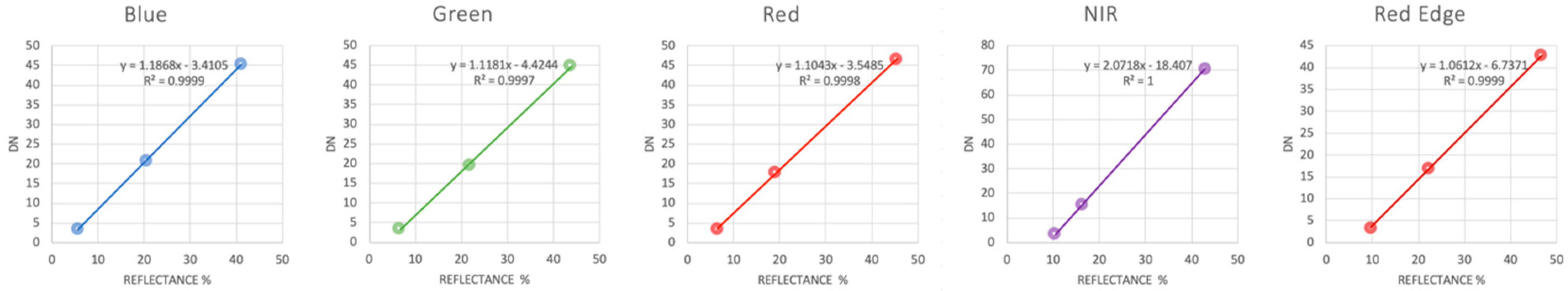
2.2. Data Collection

On 20 August 2017, image data were acquired with a RedEdge camera (Micasense, Seattle, WA, USA) (Figure 2) carried by a Tuffwing Mapper fixed-wing UAV platform (Tuffwing LLC, Boerne, TX, USA) (Figure 3) flying at 120 m AGL. The camera collected images with 1280 × 960 pixels at 7.64 cm/pixel resolution in five bands: blue (475–500 nm), green (550–565 nm), red (665–675 nm), red edge (715–725 nm), and NIR (825–860 nm). The images were taken between 11:00 and 13:00 local time on a cloud-free day, with fixed exposure settings that had been experimentally determined to be optimal for the crop, location, date, and time of day. The manual exposure settings were 0.44, 0.44, 0.44, 1.00, and 0.44 milliseconds, and gain settings were 1×, 1×, 2×, 2×, 2×, respectively for Blue, Green, Red, NIR and Rededge bands.

2.3. Data Processing

With the AGL and camera used, a 0.95-ha area was covered with each image. The overlap percentages used for UAV surveys were 80% forward-lap and 70% side-lap. Raw images were saved in tiff format with GPS and inertial measurement unit (IMU) data stored in metadata. Image mosaicking was performed in Pix4D software (Lausanne, Switzerland). When the ground control point (GCP) information was used in processing the mosaic, three to six overlapping images per location were tied, which is varied on the distance between GCPs and the edge of mosaic. All these procedures were conducted in Pix4D. The point cloud density is in the “High” option with the minimum number of matches of 3. The 3D textured mesh was generated with the default option “Medium Resolution”.

A Trimble Geoexplorer 6000 (Trimble, Sunnyvale, CA) GPS receiver was used to measure the coordinates at the center of ground control points (GCPs) in order to geo-reference the images. Geo-referencing was also performed in Pix4D, and the centers of the GCPs in each raw image were manually identified and linked to the corresponding ground truth GPS coordinates.

Three radiometric calibration references were used: light gray (≈45% reflectance), medium gray (≈20% reflectance), and dark gray (≈3% reflectance). The reflectance spectra of the calibration references were collected on the day of flight with a portable spectroradiometer (PSR+ 3500 High-Resolution Full Range Portable Spectroradiometer, Spectral Evolution, Haverhill, MA). On each calibration reference, the reflectance spectra of five points (one close to each corner and one at the center) were collected and averaged. A linear relationship between digital number (DN) values and reflectance was derived for each image band (Figure 4). Based on these relationships, each image mosaic was converted to reflectance in ENVI software (Harris Geospatial Solutions, Boulder, CO). Then the UAV mosaics were resampled at 1.0-m resolution for use by the conventional classifiers.

2.4. Classifications

Unsupervised and supervised methods were used to classify image data into two classes that indicated healthy and CRR-infested areas. The data used by each classifier in generating a classification result were only the green, red, and NIR bands from the MicaSense camera. This selection was based on three reasons. First of all, Yang et al. compared 3-band multispectral data (green, red, NIR) to hyperspectral data (475 to 845 nm) for CRR detection [9]. The spectral range of the hyperspectral data included the bandwidth range of the red edge. The results indicated both multispectral and hyperspectral images could similarly accurately distinguish the CRR-infested area, giving convincing evidence that CIR data (green, red, NIR) are sufficient to detect CRR. Second, in work preliminary to the research discussed herein, two performance comparisons based on the SVM classifier with different sets of training data were made among groups of all five bands (B, G, R, NIR, red edge), four bands (G, R, NIR, red edge), CIR (G, R, NIR), and RGB. Results indicated that CIR performed the best of all the groupings. Accuracies averaged 82.0% for five bands, 83.0% for four bands, 84.2% for CIR, and 77.2% for RGB. Finally, CIR cameras are in fairly common use, while five-band multispectral cameras are not, and a commonly applicable solution was desired. All the conventional classifications thus were generated based on CIR data, and the images were resampled to 1.0-m resolution.

2.4.1. Conventional Classification

The green, red, and NIR bands from the MicaSense camera were used as input to the classifiers, and the associated CIR images were used for visual evaluation of the classification methods. These images covered 5.68-ha, 0.42-ha, and 0.34-ha portions of the CH, SH, and WP fields, respectively (Figure 5). The 1.0-m resampled data were used with all the conventional classification methods, because standard operating procedure for this type of remote-sensing analysis involves resampled data.

All the conventional classifications were conducted in ENVI. Each image was processed individually with corresponding classification methods. One unsupervised classification method was used to classify the image data directly into two classes, and three unsupervised methods were used to classify the image data into three, five, or ten classes that were then combined into two classes based on user judgment.

K-means clustering is an unsupervised classification method that does not require labeled training data. It can classify the data based on the similarity of data in multidimensional space. The user specifies the number of clusters to be generated based on knowledge of the application; e.g., if only CRR and healthy regions were evident, only two clusters would be specified. Initially, “seeds” are generated in the data space randomly to serve as initial cluster centroids. Individual data are classified into the category associated with the closest cluster centroid. Then the centroids are recalculated based on the data in the new classes. The data are relabeled into a new class based on the updated centroid position. Iteration of these steps continues until the centroids no longer move significantly according to specified stopping criteria. In this way, most of the healthy and CRR-infected cotton can be differentiated because of the big difference between their spectral responses.

The k-means clustering method was applied to each image to generate two-class, three-class, five-class, and ten-class classification. The two-class classification was regarded as unsupervised classification, while the others were regarded as semi-supervised because class combinations were based on human expertise. In the three-class classification, Classes 1 and 2 were combined as the healthy class, and Class 3 was assigned as the CRR class. In the five-class classification, Classes 1 through 3 were combined as the healthy class, and Classes 4 and 5 were combined as the CRR class. In the ten-class classifications, Classes 1 through 6 were combined as the healthy class, and Classes 7 through 10 were combined as the CRR class.

Additionally, four supervised classification methods were used to classify the image data directly into two classes, and all used the same training regions of interest (ROIs). In each field, about 20,000 to 40,000 pixels (about 0.5% to 1.0% of an entire field) were selected for each class. The training data were uniformly distributed across the fields. Different classification rules were calculated from the training data for each supervised classification method. The classifications were then generated based on these rules. The unsupervised methods were all based on k-means classification, while the supervised methods included support vector machine (SVM), minimum distance, maximum likelihood, and Mahalanobis distance.

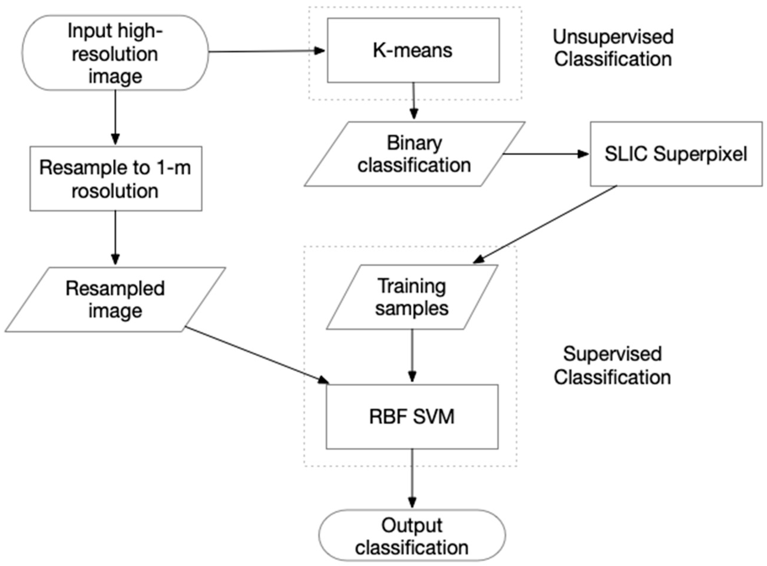
2.4.2. An Improved Semi-Supervised Classifier Based on k-means and SVM

Unsupervised clustering methods such as the k-means method can classify data without human intervention but tend to compromise on accuracy. On the other hand, supervised classification methods like SVM, do not classify the data automatically but tend to be more accurate. It was noted previously that SVM was used to differentiate disease in RS images [20]. SVM has proven capable of classifying CRR accurately with 1.0-m resolution images [5], but it requires training data typically selected by a human operator. It was proposed to use k-means to automatically select training data that would subsequently be used by SVM for complete image classification.

The idea behind combining k-means clustering with SVM was to classify pixels into CRR and healthy classes automatically while maintaining relatively high accuracy. Figure 6 makes it clear that CRR and healthy cotton generally have strong differences in reflectance. However, large numbers of pixels on the boundaries are not easily separable. Once clusters are generated, many pixels are located between the two cluster centroids, and there is overlap among the pixels. Visualization of sampled data of CRR and healthy cotton plants indicates that the data are not linearly separable either in two dimensions or three dimensions (green, red, and NIR). Unsupervised clustering such as k-means separates the data with a flat plane equidistant from cluster centroids and can cause large amounts of misclassification. Unlike k-means, which is a so-called hard classifier in that it has no tunable parameters, SVM with the RBF kernel trick can generally classify image data based on labeled training data and a flexible classification rule involving the influence distance of training data and the aforementioned penalty factor. The RBF kernel trick can map the raw dataset into a higher dimensional space for separating the data more easily, and thus make the SVM classification more accurate.

The method of combining k-means and SVM processes (KMSVM) is able to label clusters of data points automatically based on the human experience built into the code that CRR pixels have lower reflectance overall. The workflow of KMSVM is shown in Figure 7. The k-means algorithm was used to automatically select initial training data from the original high-resolution image mosaics, because the high-resolution data should have many more non-mixed pixels, enabling more precise placement of the plane between the cluster centroids. Two-class k-means clustering was thus applied to the raw ortho-mosaicked image as the first step of pre-processing to locate the distribution of CRR and healthy plants. The CRR-infected plants were assigned a digital number (DN) of 0, and the healthy plants were assigned a DN of 255. Another step was required to optimize the training data, because the ideal training data selected by the k-means algorithm must contain as much as possible of the unique features of the corresponding class and must avoid the features of the other classes. Therefore, simple linear iterative clustering (SLIC) superpixel segmentation was then applied to optimize the training data based on probability associated with the size and shape of small zones (superpixels) in the images corresponding to the expectations for individual cotton plants (Figure 8). The SLIC superpixel segmentation method was applied with a minimum superpixel compactness of 300 to the binary k-means classification data. The seeding rate for the SLIC superpixel algorithm was based on the expected size of an individual cotton plant based on row width and spacing of cotton seeds. The SLIC superpixel segmentation algorithm divided the binary image into hundreds of superpixels, calculated the mean value of DN in each superpixel, and reassigned the mean value as the new DN of each superpixel. A new DN value larger than 243 meant the segment contained more than 95% pixels labeled as healthy in the training dataset. On the other hand, DN values smaller than 12 meant 95% of the classified infested area in the segment was labeled as CRR in the training dataset. After this step, superpixels were assigned as either CRR or healthy in order to train the SVM classifier. The RBF SVM algorithm was then used on the resampled 1.0-m data to execute the final classification.

2.4.3. An Improved Classification Based on k-means Segmentation

The k-means segmentation (KMSEG) algorithm was based on k-means clustering and morphological processes. The addition of morphological processes was expected to mitigate misclassifications associated with non-seeded areas resulting from a planter malfunction. These areas are commonly misclassified as CRR zones, but their rectangular shape can be exploited to better classify them. The workflow of KMSVM is shown in Figure 9. The images were first classified with k-means, and then dilation and erosion were applied to the k-means classification result in order to segment larger CRR zones. UAV RS provides high-resolution image data, but more irrelevant data like pixels of bare soil between planting rows are introduced (Figure 10). Once the two-class k-means classification was generated based on a UAV high-resolution image mosaic, the bare soil between planting rows was classified as CRR. In conventional classification approaches, to avoid the effects of bare soil between planting rows, the image resolution is downgraded so that the pixels of plants and gaps between rows are aggregated. A shortcoming of this process is that a large amount of information is lost with the decreasing image resolution, especially at the boundaries between infected and uninfected regions. The KMSEG method generates the classification directly on the original high-resolution image mosaics and then smooths the classification result through a morphological closing process. A 3 × 3 filter was used for dilation in the healthy cotton class to fill the gaps between rows. Then, erosion of the healthy cotton class was conducted with the same size filter to shrink the class and neutralize the influence of dilation at the boundaries between CRR and healthy cotton regions. This morphological closing procedure aims to remove small or narrow bare soil areas. Five iterations each of dilation and erosion were used to ensure boundaries between classes were not affected. Finally, a morphological opening, erosion followed by dilation, was conducted in the same number of iterations, which cleaned the small healthy areas inside of infected areas.

2.5. Accuracy Assessment

Accuracy assessment is an indispensable procedure of image classification [44,45].A ground-truth map was used to assess the accuracy of classifications. The ground-truth map was drawn manually according to collected GPS coordinates and the following protocols:

(a)

A region with more than 10 adjacent cotton plants infected with CRR was marked as a CRR-infested region.

(b)

In a CRR-infested area, a region with more than 10 adjacent healthy cotton plants was regarded as a non-infested area.

A digitizer and graphic pad were used in this procedure. An expert in RS and plant pathology used experience and judgment to delineate infested areas. The generated map was classified into two values, ‘0’ (healthy) and ‘1’ (CRR) (Figure 11).

The classifications derived from the various classifiers were also converted to a binary map to test their accuracy against the human expert classification. As in the ground-truth map, the healthy area is represented by ‘0’ and the infested area is represented by ‘1’. When the two maps were overlaid, the intersecting (i.e., correctly classified) parts were assigned a value of ‘1’are, while the non-intersecting (i.e., misclassified) parts were assigned a value of ‘0’.

To assess the accuracy of classifications, the confusion matrix including agreement, omission error, commission error, and overall accuracy was generated. An error of omission represents pixels that belong to a class but are not classified into that class. For instance, the omission of CRR means CRR infested areas fail to be classified as CRR. This error is termed producer’s accuracy. Error of commission represents pixels which belong to one class but are classified into another class. For example, the commission error of CRR means healthy cotton plants are classified as CRR. This error is termed user’s accuracy.

For an accurate classification, both omission and commission errors should be at a low level. A high omission error of the CRR-infested class means that a large number of CRR-infested areas are classified healthy. Contrarily, a high commission error of the infested class means many healthy plants are misclassified as CRR-infected plants. Compared with the omission of the CRR-infested class, the commission of the CRR-infested class is more tolerable, because the CRR-infested area may extend or shrink year by year, and slight over-application of fungicide is more likely to guarantee an effective treatment result.

3. Results

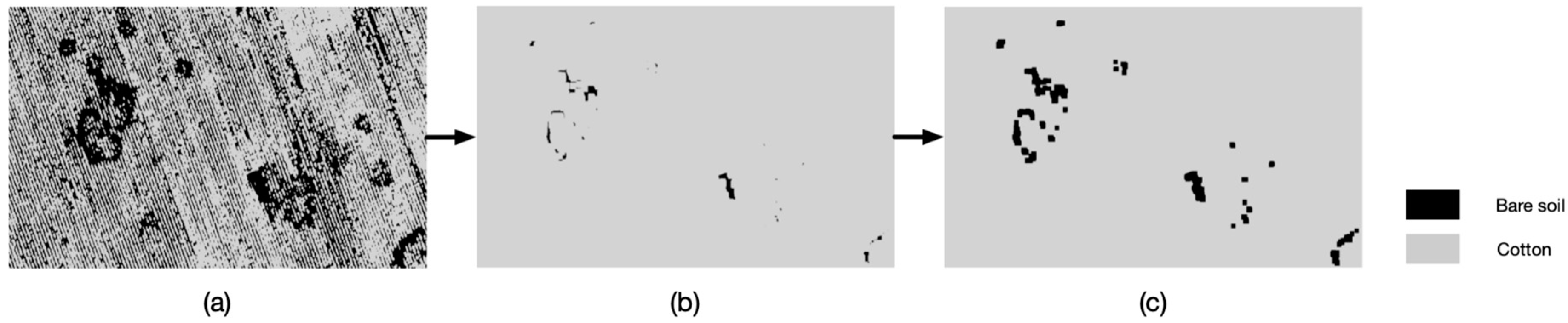
3.1. The Newly Proposed Classification Methods

Thirty confusion matrices corresponding to the ten classifiers and the three cotton fields (CH, WP, and SH) were developed and compared.

Table 1. A confusion matrix of k-means support vector machine (SVM) regional classification for Chase field.

Overall accuracy		90.69%
Kappa coefficient		0.7277
	Class types determined from the reference source (Ground-truth)				Commission	Omission
Class types determined from classified map		Infested plants	Healthy plants	Totals
	Infested plants	2157162	684748	2841910	24.09%	18.24%
	Healthy plants	481191	9205114	9686305	4.97%	6.92%
	Totals	2638353	9889862	12528215

and

Table 2. Confusion matrix of k-means segmentation regional classification for Chase field.

Overall accuracy		92.63%
Kappa coefficient		0.7786
	Class types determined from reference source (Ground-truth)				Commission	Omission
Class types determined from classified map		Infested plants	Healthy plants	Totals
	Infested plants	2182161	467623	2649784	17.65%	17.29%
	Healthy plants	456192	9422239	9878431	4.62%	4.73%
	Totals	2638353	9889862	12528215

are detailed examples of the confusion matrix for KMSVM and KMSEG in the CH field. The results from all 30 confusion matrices are summarized in

Table 3. The summarized results of accuracy comparison between unsupervised, combined-unsupervised, supervised classifications, and proposed automatic regional classifications. Three cotton fields were used to evaluate the methods of classification between healthy and cotton root rot (CRR) infested field areas.

		Overall Accuracy					Kappa Coefficient
		CH	WP	SH	Mean	Std. Dev.	CH	WP	SH	Mean	Std. Dev.
U	2-class k-means	78.60%	78.76%	81.44%	79.60%a	1.60%	0.5106	0.4527	0.6162	0.5265A	0.0829
C-U	3 to 2-class k-means	88.89%	87.26%	79.45%	85.20%ab	5.05%	0.6868	0.5751	0.5392	0.6004A	0.0770
	5 to 2-class k-means	88.67%	88.81%	83.49%	86.99%ab	3.03%	0.6085	0.5293	0.6452	0.5943A	0.0592
	10 to 2-class k-means	90.97%	88.01%	81.14%	86.71%ab	5.04%	0.6986	0.5885	0.5911	0.6261A	0.0628
S	SVM	92.02%	78.66%	87.48%	86.05%ab	6.79%	0.7587	0.4481	0.7345	0.6471A	0.1728
	Minimum distance	88.12%	86.14%	82.79%	85.68%ab	2.69%	0.6753	0.5604	0.6346	0.6234A	0.0583
	Maximum likelihood	91.71%	77.92%	87.65%	85.76%ab	7.09%	0.7498	0.4419	0.7422	0.6446A	0.1756
	Mahalanobis distance	89.60%	87.13%	86.27%	87.67%ab	1.73%	0.7076	0.5764	0.7144	0.6661A	0.0778
PA	KMSVM	90.69%	84.47%	88.15%	87.77%ab	3.13%	0.7277	0.6048	0.7494	0.6940A	0.0780
	KMSEG	92.62%	85.80%	87.06%	88.49%b	3.63%	0.7786	0.6428	0.7379	0.7198A	0.0697
		Error of Commission (CRR class)					Error of Omission (CRR class)
		CH	WP	SH	Mean	Std. Dev.	CH	WP	SH	Mean	Std. Dev.
U	2-class k-means	50.43%	56.88%	27.16%	44.82%a	15.63%	7.84%	14.10%	18.00%	13.31%A	5.13%
C-U	3 to 2-class k-means	30.04%	40.17%	17.43%	29.21%ab	11.39%	17.22%	28.28%	41.43%	28.98%BCD	12.12%
	5 to 2-class k-means	14.26%	24.23%	19.36%	19.28%ab	4.99%	44.58%	51.63%	25.30%	40.50%D	13.63%
	10 to 2-class k-means	10.85%	37.51%	21.20%	23.19%ab	13.44%	34.95%	29.83%	30.73%	31.84%CD	2.73%
S	SVM	18.50%	57.07%	16.18%	30.58%ab	22.97%	19.66%	15.04%	16.69%	17.13%AB	2.34%
	Minimum distance	32.90%	43.70%	22.15%	32.92%ab	10.78%	14.48%	24.71%	23.19%	20.79%ABC	5.52%
	Maximum likelihood	19.38%	57.88%	18.53%	31.93%ab	22.48%	20.17%	13.23%	12.39%	15.26%AB	4.27%
	Mahalanobis distance	28.74%	40.79%	20.73%	30.09%ab	10.10%	15.18%	26.86%	13.25%	18.43%ABC	7.36%
PA	KMSVM	24.09%	32.34%	9.26%	21.90%ab	11.70%	18.24%	25.17%	9.97%	17.79%ABC	7.61%
	KMSEG	17.64%	7.46%	23.30%	16.13%b	8.03%	17.29%	11.95%	5.09%	11.44%A	6.12%

Note: U stands for unsupervised, C-U stands for combined-unsupervised, S stands for supervised, PA stands for proposed automatic. Letters a, b and c (A, B and C) in Column Mean indicate statistical different groups (α = 0.05, Duncan test).

. KMSVM had consistent performance in all three fields. The overall accuracies for KMSVM in the CH, WP, and SH fields were 90.69%, 84.47%, and 88.15%, respectively. Table 1 shows that 12,528,215 pixels in CH were evaluated in the accuracy assessment. Exactly 684,758 pixels (24.09%) of healthy plants were overclassified into the CRR-infested class. Additionally, 481,191 pixels (18.24%) of CRR-infected plants failed to be detected. Finally, 9,205,114 pixels of healthy plants and 2,157,162 pixels of infected plants were correctly classified with an overall accuracy of 90.69% and a kappa coefficient of 0.7277, indicating substantial agreement (0.61–0.80) with the true data [46,47]. The KMSVM classification results are at about the same accuracy level as the supervised classifications (Table 3).

The same dataset was used to evaluate the KMSEG method (Table 2). KMSEG had better performance than KMSVM in overall accuracy, kappa coefficient, error of commission and error of omission. For the CH field, the overall accuracy (92.63%) was as good as those for the supervised classifications (Table 1 and Table 3), and the commission error (17.65%) and omission error (17.29%) were relatively low.

3.2. Comparison Between Newly Proposed and Conventional Classification Methods

The conventional unsupervised and supervised classification methods were compared with the newly proposed methods (Table 3). The two-class k-means clustering method was able to generate CRR distribution maps automatically, similar to KMSVM and KMSEG from an automation perspective. However, the average accuracy of 79.60% and the average kappa coefficient of 0.5265 were lower than those for KMSVM (87.77% and 0.6940) and KMSEG (88.49% and 0. 7198). The error of omission of 13.31% was acceptable, but the error of commission was 44.82%, indicating that nearly half of the estimated CRR area was over-classified. The two proposed methods performed significantly better than two-class k-means (α = 0.05) in terms of commission error. However, the omission errors were similar between two-class k-means and the two proposed methods.

The combined three-class, five-class, and 10-class k-means clustering methods achieved accuracies of 85.20%, 86.99%, and 86.71%, respectively, indicating that generating more classes for k-means clustering improved classification results and reduced the error of commission to the level of the proposed methods. However, the procedure of combining classes required human input and knowledge of relevant classes, making these methods less desirable than the proposed methods from the perspective of automation. Compared with the two-class k-means classification, the combined multi-class k-means classifications had better results in overall accuracy, kappa coefficient, and error of commission, but the differences were not significant (α = 0.05). For the error of omission, the two-class k-means classification performed significantly better than the combined multi-class k-means classifications.

The performance of the four supervised classifications was generally good. The overall accuracies for SVM, minimum distance, maximum likelihood, and Mahalanobis distance were 86.05%, 85.68%, 85.76%, and 87.67%, respectively. The respective errors of commission were 30.58%, 32.92%, 31.93%, and 30.09%, and the respective errors of omission were 17.13%, 20.79%, 15.26%, and 18.43%. Compared with KMSVM and KMSEG, the supervised classification methods had similar performance in terms of accuracy and kappa coefficient. However, the errors of commission of the supervised classifications were almost twice those of the proposed methods. And the errors of omission were also higher than those of the proposed methods. Figure 12 shows the classification results of eight conventional and two proposed classifiers for the CH field. The CRR-infested zone is in dark gray, and the healthy zone is in light gray. Each classification in Figure 10 has a corresponding error map that shows the difference between the classification and the ground truth map. The omission error of CRR is in cyan and represents misdetection of CRR, while the commission error of CRR is in pink and represents overclassified CRR. The classification results of the CH field indicated that all the supervised classifications, especially SVM (Figure 12e), maximum likelihood (Figure 12g), and Mahalanobis distance (Figure 12h), had large commission errors (see stripes) at the northwest corner of the CH field where non-seeded areas were wrongly classified into CRR. KMSVM (Figure 12i) also had a similar misclassification at the northwest corner of the CH field.

A scatterplot of errors of commission versus errors of omission is shown in Figure 13. The shorter the distance from the classifier to the origin, the less overall error the classifier had. The error data points of the conventional classifiers fell roughly along a common curve, while the two proposed classification methods, which took advantage of the higher resolution of the UAV image mosaics, were much closer to the origin.

4. Discussion

An idealized goal of developing CRR detection methods is to enable the uploading of raw UAV images to a cloud server or farm computer for automatic image mosaicking and processing and then to convert the classified map to a prescription map as the final product. The prescription map would be loaded to the control system for the planter to apply fungicide automatically at planting. The entire process including image classification would ideally be automatic or at least semi-automatic. Although supervised classification and combined unsupervised classification have good classification results, they all require human expertise, making it impossible to process the data automatically. On the other hand, unsupervised classification with the two proposed methods, KMSVM and KMSEG, meets the requirement of automation.

A dataset containing roughly 584,000 pixels of data sampled from two different fields was used to analyze the features of CRR data. Statistical analysis of CRR and healthy sample data indicates that the DN values of both CRR and healthy cotton follow a bell-shaped distribution in green, red, and NIR bands (Figure 14). Assuming the distance between two cluster centroids is normalized to 100%, the data closer than 50%, 33%, and 25% to the closer centroid were considered in groups with respect to classification accuracy. The 50% group was correctly classified in the range of 42% to 58%. The 33% group was correctly classified in the range of 77% to 96%. Finally, the 25% group was correctly classified in the range of 85% to 100%. Selecting training data by using k-means classification directly may cause overfitting in classification. Selecting training data around the cluster centroid within 33% of the distance between two cluster centers could be a strategy to automatically select training data, but this may lead to underfitting. Therefore, SLIC superpixel segmentation was introduced to improve the fit associated with the training data. The non-linear separable feature of the data is one of the reasons that the conventional unsupervised classifier was not able to directly achieve a good classification result.

Combined multi-class k-means methods were able to improve the accuracy of the classification compared to the two-class k-means methods. More classes could lead to higher accuracy theoretically, because the boundary effects could be reduced with the increasing number of classes. However, the decision criterion for class combination was subjective. Considering the combined five-class k-means classification as an example, combining Classes 1 and 2 to the CRR class and Classes 3, 4 and 5 to the healthy class led to very similar accuracy as compared to combining Classes 1, 2 and 3 to CRR and Classes 4 and 5 to healthy. The first combination had high omission error, while the second combination had high commission error, indicating that Class 3 included both CRR and healthy areas. Rigid separation of classes caused inaccurate and subjective results.

The conventional supervised classifications and KMSVM had difficulty distinguishing CRR-infected plants from non-seeded areas. The unsupervised methods also had a similar issue, but it was not as severe as with the supervised methods. This issue occurred because the spectral features of CRR plants and bare soil were similar. Using only spectral information led to misclassification. However, KMSEG avoided this issue by making use of the morphology of how CRR presents itself in the field. CRR-infested areas are generally in circular or ring shapes [3], but non-seeded areas caused by planter mechanical failure are normally in strips with bare soil. Taking the CH field as an example, there is a seeding error at the northeast corner (Figure 12). The bare soil area caused by mis-seeding is long and narrow. The morphological closing transformation procedure in KMSEG tended to aggregate the strip-shaped bare soil pixels (Figure 15). This is one reason why KMSEG achieved the lowest error of commission among all methods.

An ideal classifier for detecting CRR should have not only good overall accuracy but should also keep the omission and commission errors of the CRR class as low as possible. Commission error indicates over-classification; i.e., larger commission error means more fungicide treatment area, which wastes fungicide and increases environmental risk. To the contrary, a large omission error causes the under-application of fungicide to infested areas, thus reducing cotton yield and quality. In future studies, image classification should be optimized to minimize misclassified areas while reducing application costs.

A principal benefit of using the high-resolution imagery of UAVs is that it may ultimately enable highly precise application of fungicide to protect cotton plants from CRR, but for this research it also enabled highly precise ground truth maps to be used for accuracy assessment. The classifications were evaluated based on all image pixels in a specific zone instead of randomly sampled points, making the result more robust. However, the pixels at a boundary of two classes could decrease the overall accuracy more easily in some scenarios (Figure 16). This phenomenon is known as the boundary effect, and while it could influence the absolute accuracy somewhat, it was not expected to affect the comparisons between classifiers. The results (Table 3) basically agreed with Yang’s research [5] in that the combined unsupervised classification methods were as good as the supervised classification methods. The maximum likelihood classifier was slightly better than minimum distance in overall accuracy. The SVM had the best overall accuracy among all the supervised classifiers. But overall, the supervised classifiers all performed well and showed no major differences.

Two morphological operations were used with the high-resolution data to account for shape in the proposed classification methods: opening and closing was used in KMSEG to eliminate non-seeded areas, and superpixel analysis was used in KMSVM to enable specific focus on cotton plants. While these spatially focused operations can potentially account for the different look of other causes of plant death and wilt, the image analysis done here assumes CRR to be the major cause of wilted and dead plants, based on historical knowledge that CRR is in the field, and sampling of individual plants verifies it, along with the commonly round patterns in the field.

The particular innovations were fully automated classifiers, classifiers that perform well with high-resolution UAV data, and the inclusion of spatial information in the classifiers. We believe the proposed classification methods can be useful in other disease and pest detection contexts. However, it must be noted that the proposed methods were designed specifically for use in CRR, in which in-season mitigation is not possible. The goal with CRR is to allow the disease to take its course so the full-scale of the disease pattern can be measured. Once the disease pattern is clearly delineated at high resolution, fungicide can be applied during planting with extreme precision to minimize cost and environmental risk.

While a fixed-wing UAV was used in this work, rotary-wing UAVs are more common today, particularly in research applications. We used a fixed-wing aircraft because we desire to develop a data-collection and classification system that may be potentially practical on-farm, and thus covering large fields quickly is critical. Because fixed-wing aircraft generate lift from forward speed, they are more efficient at staying in the air over large areas and can cover a 100-acre field in a typical 20-minute flight, including adequate overlap for the orthomosaicking process.

5. Conclusions

This study compared multiple conventional classifiers and proposed two improved automatic classifiers, KMSVM and KMSEG, to classify CRR-infected and healthy plants in cotton fields. KMSVM is a self-labeling machine learning classifier, while KMSEG emphasizes morphological processes, and both of these were used in a way that took advantage of the high resolution inherent in UAV images. All the classifiers were evaluated based on two criteria, automation and accuracy. The two proposed methods performed better in terms of accuracy than the conventional classifiers and could be implemented automatically. In particular, the KMSEG classifier had the best performance in terms of overall accuracy (88.39%), Kappa coefficient (0.7198), error of commission (16.13%), and error of omission (11.44%). The two-class unsupervised classification had the lowest overall accuracy (79.60%) and the highest error of commission (44.82%), but it had the advantage in automation over the supervised classifications. The combined multi-class unsupervised classifications and supervised classifications had relatively good accuracy (85.2% to 87.67%) but required human intervention. Overall, the proposed methods proved superior in classifying high-resolution UAV images into healthy and diseased areas at roughly the level of a single plant.

References

1. Pammel, L.H. Root rot of cotton or “cotton blight”. Texas Agric. Exp. Stn. Ann. Bull. 1888, 4, 50–65. [Google Scholar]
2. Smith, H.E.; Elliott, F.C.; Bird, L.S. Root rot losses of cotton can be reduced. Misc. Publ. Tex. Agric. Exp. Stn. No. 361 1962. [Google Scholar]
3. Yang, C.; Odvody, G.N.; Fernandez, C.J.; Landivar, J.A.; Minzenmayer, R.R.; Nichols, R.L.; Thomasson, J.A. Monitoring cotton root rot progression within a growing season using airborne multispectral imagery. J. Cotton Sci. 2014, 93, 85–93. [Google Scholar]
4. Smith, R. South Texas Cotton Root Rot Draws Study. Available online: https://www.farmprogress.com/south-texas-cotton-root-rot-draws-study (accessed on 23 September 2019).
5. Yang, C.; Odvody, G.N.; Fernandez, C.J.; Landivar, J.A.; Minzenmayer, R.R.; Nichols, R.L. Evaluating unsupervised and supervised image classification methods for mapping cotton root rot. Precis. Agric. 2015, 16, 201–215. [Google Scholar] [CrossRef]
6. Isakeit, T.; Minzenmayer, R.R.; Drake, D.R.; Morgan, G.D.; Mott, D.A.; Fromme, D.D.; Multer, W.L.; Jungman, M.; Abrameit, A. Fungicide management of cotton root rot (Phymatotrichopsis omnivora): 2011 results. In Proceedings of the Beltwide Cotton Conference, San Antonio, TX, USA, 3–6 January 2012; pp. 235–238. [Google Scholar]
7. Isakeit, T.; Minzenmayer, R.; Abrameit, A.; Moore, G.; Scasta, J.D. Control of phymatotrichopsis root rot of cotton with flutriafol. In Proceedings of the Beltwide Cotton Conference, San Antonio, TX, USA, 9 January 2013; pp. 200–203. [Google Scholar]
8. Isakeit, T. Management of cotton root rot. In Proceedings of the Beltwide Cotton Conference, San Antonio, TX, USA, 3–5 January 2018; p. 43. [Google Scholar]
9. Yang, C.; Everitt, J.H.; Fernandez, C.J. Comparison of airborne multispectral and hyperspectral imagery for mapping cotton root rot. Biosyst. Eng. 2010, 107, 131–139. [Google Scholar] [CrossRef]
10. Chenhai, Y.; Minzenmayer, R.R.; Extension, T.A.; Nichols, R.L.; Incorporated, C.; Isakeit, T.; Thomasson, J.A.; Fernandez, C.J.; Landivar, J.A. Monitoring cotton root rot infection in fungicide-treated cotton fields using airborne imagery. In Proceedings of the Beltwide Cotton Conferences, New Orleans, LA, USA, 6–8 January 2013. [Google Scholar]
11. Taubenhaus, J.J.; Ezekiel, W.N.; Neblette, C.B. Airplane photography in the study of cotton root rot. Phytopathology 1929, 19, 1025–1029. [Google Scholar]
12. Nixon, P.R.; Lyda, S.D.; Heilman, M.D.; Bowen, R.L. Incidence and control of cotton root rot observed with color infrared photography. MP Tex. Agric. Exp. Stn. 1975. [Google Scholar]
13. Nixon, P.R.; Escobar, D.E.; Bowen, R.L. A multispectral false-color video imaging system for remote sensing applications. In Proceedings of the 11th Biennial Workshop on Color Aerial Photography and Videography in the Plant Sciences and Related Fields, Weslaco, TX, USA, 1 september 1987; pp. 295–305. [Google Scholar]
14. Yang, C.; Fernandez, C.J.; Everitt, J.H. Mapping phymatotrichum root rot of cotton using airborne three-band digital imagery. Trans. ASAE 2005, 48, 1619–1626. [Google Scholar] [CrossRef]
15. Song, X.; Yang, C.; Wu, M.; Zhao, C.; Yang, G.; Hoffmann, W.C.; Huang, W. Evaluation of Sentinel-2A satellite imagery for mapping cotton root rot. Remote Sens. 2017, 9, 906. [Google Scholar] [CrossRef] [Green Version]
16. Yang, C.; Greenberg, S.M.; Everitt, J.H.; Fernandez, C.J. Assessing cotton defoliation, regrowth control and root rot infection using remote sensing technology. Int. J. Agric. Biol. Eng. 2011, 4, 1–11. [Google Scholar]
17. Huang, Y.; Thomson, S.J.; Brand, H.J.; Reddy, K.N. Development and evaluation of low-altitude remote sensing systems for crop production management. Int. J. Agric. Biol. Eng. 2016, 9, 1–11. [Google Scholar]
18. Easterday, K.; Kislik, C.; Dawson, T.E.; Hogan, S.; Kelly, M. Remotely sensed water limitation in vegetation: Insights from an experiment with unmanned aerial vehicles (UAVs). Remote Sens. 2019, 11, 1853. [Google Scholar] [CrossRef] [Green Version]
19. Zhou, X.; Zheng, H.B.; Xu, X.Q.; He, J.Y.; Ge, X.K.; Yao, X.; Cheng, T.; Zhu, Y.; Cao, W.X.; Tian, Y.C. Predicting grain yield in rice using multi-temporal vegetation indices from UAV-based multispectral and digital imagery. ISPRS J. Photogramm. Remote Sens. 2017, 130, 246–255. [Google Scholar] [CrossRef]
20. Albetis, J.; Duthoit, S.; Guttler, F.; Jacquin, A.; Goulard, M.; Poilvé, H.; Féret, J.B.; Dedieu, G. Detection of Flavescence dorée grapevine disease using unmanned aerial vehicle (UAV) multispectral imagery. Remote Sens. 2017, 9, 308. [Google Scholar] [CrossRef] [Green Version]
21. Romero, M.; Luo, Y.; Su, B.; Fuentes, S. Vineyard water status estimation using multispectral imagery from an UAV platform and machine learning algorithms for irrigation scheduling management. Comput. Electron. Agric. 2018, 147, 109–117. [Google Scholar] [CrossRef]
22. Mattupalli, C.; Moffet, C.A.; Shah, K.N.; Young, C.A. Supervised classification of RGB Aerial imagery to evaluate the impact of a root rot disease. Remote Sens. 2018, 10, 917. [Google Scholar] [CrossRef] [Green Version]
23. Duan, B.; Fang, S.; Zhu, R.; Wu, X.; Wang, S.; Gong, Y.; Peng, Y. Remote estimation of rice yield with unmanned aerial vehicle (uav) data and spectral mixture analysis. Front. Plant Sci. 2019, 10, 204. [Google Scholar] [CrossRef] [Green Version]
24. Herrmann, I.; Bdolach, E.; Montekyo, Y.; Rachmilevitch, S.; Townsend, P.A.; Karnieli, A. Assessment of maize yield and phenology by drone-mounted superspectral camera. Precis. Agric. 2020, 21, 51–76. [Google Scholar] [CrossRef]
25. Cai, Y.; Guan, K.; Nafziger, E.; Chowdhary, G.; Peng, B.; Jin, Z.; Wang, S.; Wang, S. Detecting In-season crop nitrogen stress of corn for field trials using UAV-and cubesat-based multispectral sensing. IEEE J. Sel. Top. Appl. Earth Obs. Remote Sens. 2019, 12, 5153–5166. [Google Scholar] [CrossRef]
26. Zhang, L.; Zhang, H.; Niu, Y.; Han, W. Mapping maizewater stress based on UAV multispectral remote sensing. Remote Sens. 2019, 11, 605. [Google Scholar] [CrossRef] [Green Version]
27. Su, J.; Liu, C.; Coombes, M.; Hu, X.; Wang, C.; Xu, X.; Li, Q.; Guo, L.; Chen, W. Wheat yellow rust monitoring by learning from multispectral UAV aerial imagery. Comput. Electron. Agric. 2018, 155, 157–166. [Google Scholar] [CrossRef]
28. Matese, A.; Toscano, P.; Di Gennaro, S.F.; Genesio, L.; Vaccari, F.P.; Primicerio, J.; Belli, C.; Zaldei, A.; Bianconi, R.; Gioli, B. Intercomparison of UAV, aircraft and satellite remote sensing platforms for precision viticulture. Remote Sens. 2015, 7, 2971–2990. [Google Scholar] [CrossRef] [Green Version]
29. Ball, G.H.; Hall, D.J. ISODATA, a Novel Method of Data Analysis and Pattern Classification; Stanford Research Institute: Menlo Park, CA, USA, 1965. [Google Scholar]
30. Hartigan, J.A.; Wong, M.A. Algorithm AS 136: A K-means clustering algorithm. J. R. Stat. Soc. Ser. C Appl. Stat. 1979, 28, 100–108. [Google Scholar] [CrossRef]
31. Breiman, L. Random forests. Mach. Learn. 2001, 45, 5–32. [Google Scholar] [CrossRef] [Green Version]
32. Aha, D.W.; Kibler, D.; Albert, M.K. Instance-based learning algorithms. Mach. Learn. 1991, 6, 37–66. [Google Scholar] [CrossRef] [Green Version]
33. Burges, C.J.C. A tutorial on support vector machines for pattern recognition. Data Min. Knowl. Discov. 1998, 2, 121–167. [Google Scholar] [CrossRef]
34. Chang, C.C.; Lin, C.J. LIBSVM: A Library for support vector machines. ACM Trans. Intell. Syst. Technol. 2011, 2, 27. [Google Scholar] [CrossRef]
35. Dempster, A.P.; Laird, N.M.; Rubin, D.B. Maximum likelihood from incomplete data via the EM algorithm. J. R. Stat. Soc. Ser. B 1977, 39, 1–22. [Google Scholar]
36. MacQueen, J. Some methods for classification and analysis of multivariate observations. Proc. Fifth Berkeley Symp. Math. Stat. Probab. 1967, 1, 281–297. [Google Scholar]
37. De Maesschalck, R.; Jouan-Rimbaud, D.; Massart, D.L. The Mahalanobis distance. Chemom. Intell. Lab. Syst. 2000, 50, 1–18. [Google Scholar] [CrossRef]
38. Pal, M.; Mather, P.M. Support vector machines for classification in remote sensing. Int. J. Remote Sens. 2005, 26, 1007–1011. [Google Scholar] [CrossRef]
39. Mountrakis, G.; Im, J.; Ogole, C. Support vector machines in remote sensing: A review. ISPRS J. Photogramm. Remote Sens. 2011, 66, 247–259. [Google Scholar] [CrossRef]
40. Gong, P.; Howarth, P.J. Land-use classification of SPOT HRV data using a cover-frequency method. Int. J. Remote Sens. 1992, 13, 1459–1471. [Google Scholar] [CrossRef]
41. Lu, D.; Weng, Q. A survey of image classification methods and techniques for improving classification performance. Int. J. Remote Sens. 2007, 28, 823–870. [Google Scholar] [CrossRef]
42. Fauvel, M.; Benediktsson, J.A.; Chanussot, J.; Sveinsson, J.R. Spectral and spatial classification of hyperspectral data using SVMs and morphological profiles. IEEE Trans. Geosci. Remote Sens. 2008, 46, 3804–3814. [Google Scholar] [CrossRef] [Green Version]
43. Huang, X.; Weng, C.; Lu, Q.; Feng, T.; Zhang, L. Automatic labelling and selection of training samples for high-resolution remote sensing image classification over urban areas. Remote Sens. 2015, 7, 16024–16044. [Google Scholar] [CrossRef] [Green Version]
44. Congalton, R.G. A review of assessing the accuracy of classifications of remotely sensed data. Remote Sens. Environ. 1991, 37, 35–46. [Google Scholar] [CrossRef]
45. Huang, C.; Davis, L.S.; Townshend, J.R.G. An assessment of support vector machines for land cover classification. Int. J. Remote Sens. 2002, 23, 725–749. [Google Scholar] [CrossRef]
46. Landis, J.R.; Koch, G.G. The measurement of observer agreement for categorical data. Biometrics 1977, 33, 159–174. [Google Scholar] [CrossRef] [Green Version]
47. Rafieyan, V. Effect of cultural distance on translation of culture-bound texts. Int. J. Educ. Lit. Stud. 2016, 4, 67–73. [Google Scholar]
Figure 1. The study was conducted at (a) a farm in Williamson County, Texas; (b) the Chase field (CH for short) (Scale 1:10000); (c) the West Poncho field (WP for short) (Scale 1:15000); and (d) the School House field (SH for short) (Scale 1:6000).
Remotesensing 12 01310 g001
Figure 2. MicaSense RedEdge camera. It has five separate imaging sensors with specific optical filters to provide five spectral bands. The weight is 150 g and the size is 12.1 × 6.6 × 4.6 cm (4.8″ × 2.6″ × 1.8″), so it is designed well for use on small unmanned aerial vehicles (UAVs). Images are captured at rate of 1 capture/s and stored in SD card.
Remotesensing 12 01310 g002
Figure 3. Fixed-wing UAV “TuffWing UAV Mapper.” The aircraft body is made of expanded polypropylene (EPP) foam with reinforcing carbon fiber spars, so it is strong with low mass to maximize flight time. Including the Micasense RedEdge camera, the weight is about 2 kg, and the wingspan is 1218 cm. At the manufacturer-reported flying endurance of 40 min, the Tuffwing can cover 275 acres at 100 m above-ground level (AGL).
Remotesensing 12 01310 g003
Figure 4. The linear relationships between digital number (DN) value and reflectance of the calibration tiles in the MicaSense camera’s five spectral bands.
Remotesensing 12 01310 g004
Figure 5. Multispectral color infrared (CIR) images for (a) Chase field (Scale 1:3000), (b) School house field (Scale 1:1550), and (c) West Poncho field (Scale 1:2110).
Remotesensing 12 01310 g005
Figure 6. The relationships between bands in a sampled dataset along with k-means cluster centroids.
Remotesensing 12 01310 g006
Figure 7. The workflow of the proposed k-means support vector machine (KMSVM) method. KMSVM makes use of unsupervised clustering and the superpixel algorithm to select training data for SVM classification.
Remotesensing 12 01310 g007
Figure 8. A k-means classification (a) was converted to a super-pixel image (b) by using the simple linear iterative clustering segmentation method (Scale 1:700).
Remotesensing 12 01310 g008
Figure 9. The workflow of the proposed k-means segmentation (KMSEG) method. KMSEG makes use of unsupervised clustering and morphological image processing methods to classify the image.
Remotesensing 12 01310 g009
Figure 10. The cotton root rot (CRR) infested cotton shown in color-infrared composites with different resolutions: (a) 0.076 m/pixel; and (b) 1 m/pixel (Scale 1:200).
Remotesensing 12 01310 g010
Figure 11. The ground-truth map of Chase field was used for accuracy assessment (Scale 1:2800).
Remotesensing 12 01310 g011
Figure 12. Classification results of (A) 2-class k-means, (B) combined 3-class k-means, (C) combined 5-class K-means, (D) combined 10-class k-means, (E) SVM, (F) minimum distance, (G) maximum likelihood, (H) Mahalanobis distance, (I) KMSVM, and (J) KMSEG. Corresponding error maps of: (a) 2-class k-means, (b) combined 3-class k-means, (c) combined 5-class k-means, (d) combined 10-class k-means, (e) SVM, (f) minimum distance, (g) maximum likelihood, (h) Mahalanobis distance, (i) KMSVM, and (j) KMSEG. (Scale 1:9000).
Remotesensing 12 01310 g012
Figure 13. Error of commission versus error of omission for 10 classification methods. The errors of conventional classifications were distributed as a curved trend. The proposed methods KMSVM and KMSEG are superior and lie off the trend line.
Remotesensing 12 01310 g013
Figure 14. Spectral value distribution of CRR-infested and healthy plants.
Remotesensing 12 01310 g014
Figure 15. The strip-shaped bare soil pixels were effectively removed using morphological closing transformation at northeast of CH field. The (a) k-means classification was applied (Scale 1:2000) (b) dilation of healthy cotton class followed by (c) erosion of healthy cotton class.
Remotesensing 12 01310 g015
Figure 16. The pixels at the boundary of two classes could impact the accuracy. (a) The raw CIR image derived (Scale 1:200) (b) ground-truth image which could have boundary effect when compared to (c) real classification.
Remotesensing 12 01310 g016