Abstract
Rainfall-induced floods often cause significant loss of life as well as damage to infrastructure and crops. Synthetic Aperture Radar (SAR) Earth Observation Satellites (EOS) can be used to determine the extent of flooding over large geographical areas. Unlike optical sensors, SAR instruments are suitable for cloudy weather conditions, making them suitable for flood detection and mapping during extreme weather events. In this study, we explore the application of the Normalized Difference Sigma-Naught Index (NDSI) and Shannon’s entropy of NDSI (SNDSI) of Sentinel-1 data for open water flooding detection, based on automatic thresholding and Bayesian probability. The proposed methodology was tested using the floods in Sofala province, Mozambique, caused by cyclone Idai on March 14–19 of 2019. Results show that thresholding of the NDSI Vertical Transmit-Horizontal Receive (VH) can produce results with Overall Accuracy above 90%, and Kappa higher than 0.6. Considerable performance improvements were obtained by our thresholding method over the entropy of NDSI, yielding results with Kappa of 0.70–0.77. Additionally, it was found that Weibull distribution can properly describe the properties of flooded pixels within the histogram of SNDSI, which allows us to generate a flood probability raster using a Bayesian approach. The final per-pixel flooding probability is useful to indicate certainty in the classification results. The SNDSI Bayesian model produced an AUC (Area Under the Receiver Operating Characteristic Curve) of 0.93–0.97, with cross-polarized data yielding the most accurate results.
1. Introduction
Floods are one of the most common and destructive natural hazards. This phenomenon has severe effects on society and the environment: numerous human lives are lost, vast urban areas are damaged, crops and livestock perish, and waterborne diseases rise [1,2]. Every year, around 250 million people worldwide are affected by flooding, with annual average losses upwards of USD 40 billion [3]. Unfortunately, the frequency and intensity of floods have increased over the last decades due to climate change and anthropogenic influence, placing even more people at risk [4]. Therefore, it is necessary to provide accurate and reliable information about the spatial extent and location of flooding areas so decision-makers and disaster relief agencies can deliver prompt support to affected populations.
Nowadays, Earth Observation Satellites (EOS) such as Landsat 5–8 [5,6], SPOT 6–7 [7], and Sentinel 2 [8] facilitate the detection of floods over large geographical areas at a consistent time interval [9]. As long as the atmospheric conditions are suitable, optical sensors can provide good delineation of flooded areas with very high ground resolution. Nevertheless, the main disadvantage of optical sensors is that they cannot retrieve information over areas covered by thick clouds, as it is the case in much of the flooding events generated by intense precipitation [10]. This reason by itself hinders the applicability of optical imagery for rapid flood detection and monitoring.
On the other hand, active sensors such as Synthetic Aperture Radar (SAR) sensors can operate under all kinds of weather conditions, thus facilitating the detection of floods over large geographical areas at a consistent time rate over the same area [11,12,13]. SAR sensors emit microwaves and receive the signals which scattered back from the target. These microwaves are capable of penetrating cloud and rain, thus allowing for data collection under all-weather conditions at both day and nighttime [14].
Many SAR-based methods have been developed for flood extent detection. Some of these algorithms include visual interpretation [15], image segmentation [16], fuzzy classification [17,18], texture analysis [19], change detection [14], and histogram thresholding [20,21,22]. Open-water flooding is detectable in SAR intensity images because smooth water surfaces lead to specular reflection, bouncing off the SAR pulse away from the satellite. As a result, the backscattering intensity detected by the SAR sensor is very low or nonexistent [23].
In this study, we develop a novel framework that combines multiple techniques in SAR intensity-derived products for open water flood proxy mapping. The first approach requires the computation of a normalized scattering difference between reference and event images, acquired before and during the flooding event. Changes in backscattering intensity are a consequence of alterations in the target characteristics (e.g., roughness and dielectric properties), and by normalizing the difference in backscattering, it is possible to highlight areas where significant decrease and increase in intensity have occurred. The use of the normalized difference facilitates the exclusion of water-like (e.g., smooth) land cover types such as airplane runways or large parking lots. Considering that image thresholding has been found to be a simple, robust, and computationally efficient method for flood detection, we implemented an automatic mechanism to calculate the threshold based on the histogram of the normalized scattering image, which is then applied to classify open water inundated zones.
Secondly, we extract texture information within the normalized difference image. This process involves the estimation of Shannon’s entropy for pixel values within a sliding moving window. By considering the texture of targets whose properties have changed between two SAR acquisitions, we are able to identify inundated areas and also reduce the salt-and-pepper noise inherent in pixel-based classification methods. Furthermore, the probability for each pixel in the texture image of being flooded is calculated through a Bayesian approach and curve-fitting of the histogram. The generated probabilistic map allows us to have a non-binary flood probability map on which several flood confidence thresholds for the mapped affected areas can be set.
2. Case Study
In this study, we focus on the large flooding triggered by Cyclone Idai in Sofala province, Mozambique, on 14–19 March 2019. On 14 March, Cyclone Idai made landfall over the southern African nations of Malawi, Mozambique, and Zimbabwe as a category 2 storm. The storm devastated Mozambique coastal cities, especially the city of Beira, with winds speed of 175 km h−1. At the time of landfall, Cyclone Idai caused the storm surge of up to 4 meters around the Pungwe River delta [24], on the east coast of Mozambique. As the storm moved inland at a slow pace, it brought extreme precipitation into Sofala and Manica provinces. Data from NASA Global Precipitation Mission (GPM) revealed that over the course of five days, some areas in Mozambique received more than 600 mm of accumulated rainfall [25]. The intense precipitation combined with strong winds generated large flash floods, killing at least 650 people and affecting almost 1.8 million people in Mozambique alone, where the total estimated economic loss amounted to USD$ 1.4 billion [26].
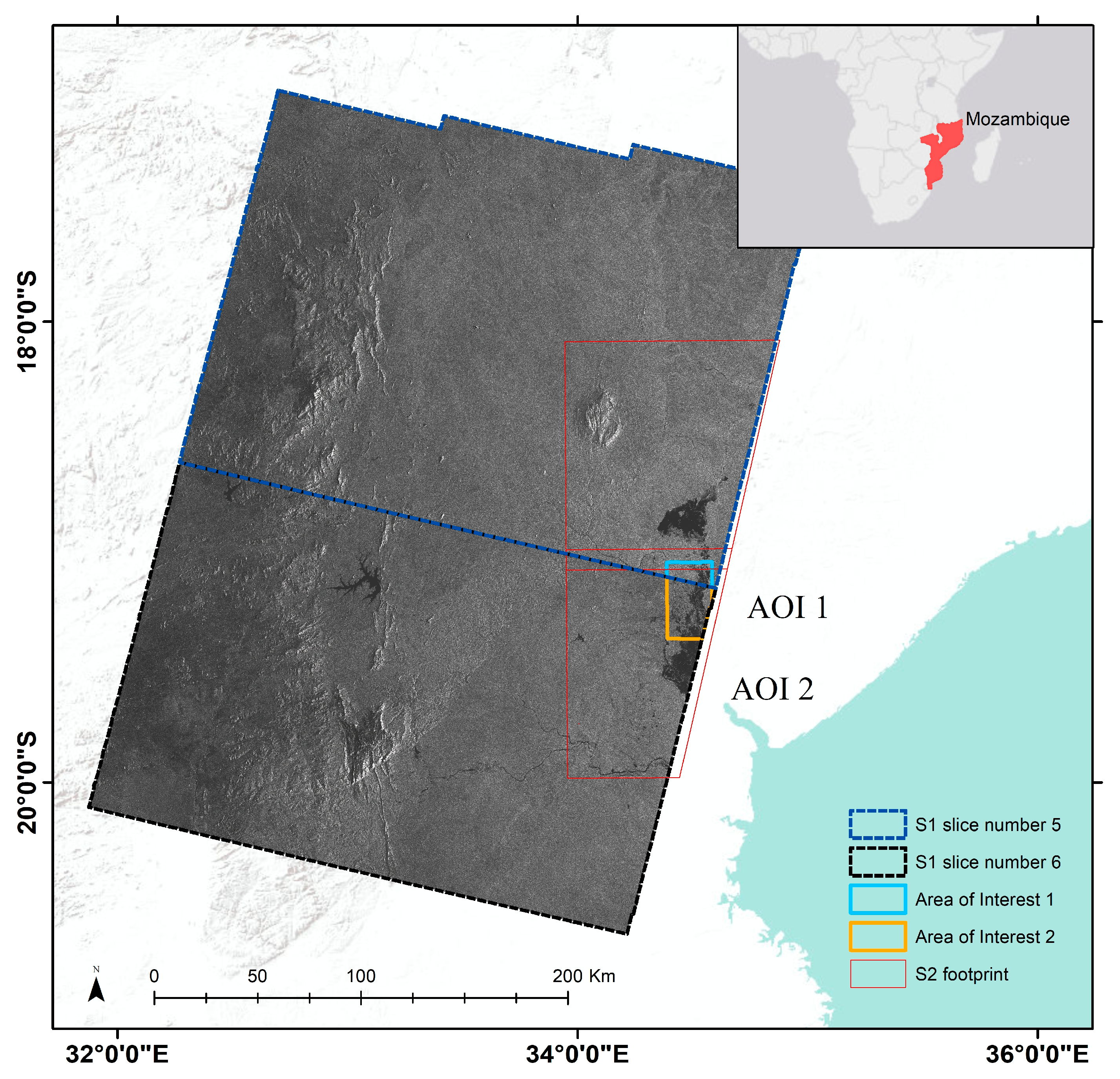
As shown in Figure 1, two Areas of Interest (AOI) have been selected, one for each Sentinel-1 image with a unique relative start orbit number. The extent of AOI 1 and AOI 2 is approximately 200 and 400 km2, respectively. In terms of land cover, more than 60% of AOI is covered by open forest and closed deciduous needle leaf forest, based on Copernicus Global Land Cover product [27]. AOI 2 presents a more heterogeneous landscape where the most predominant type is open forest, making up to 35% of the area.
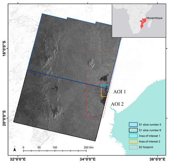
Figure 1.
Selected Areas of Interest (AOI 1 and AOI 2), and footprint of Sentinel-1 images from relative orbit 79 slices 5 and 6, and Sentinel-2 scenes.
The selected AOI present sizeable samples of inundated and non-inundated pixels, which are required to describe the characteristics of those two classes over the entire image. Moreover, we selected two AOI to check the consistency of the proposed method when applied to independent Sentinel-1 scenes.
3. Materials
3.1. Sentinel 1
The Sentinel-1 (S1) mission from the European Space Agency (ESA) consists of a pair of twin near-polar sun-synchronous satellites (S1A and S1B) equipped with Synthetic Aperture Radar (SAR) sensors that were launched in April of 2014 and 2016, respectively [28]. S1 data are acquired by a C-band sensor at a frequency of 5.407 GHz with an incidence angle in the range of 20–45° [29]. With two orbiting satellites, the S1 mission can gather data every three days in equatorial areas and more frequently at higher latitudes. The default acquisition mode over land is Interferometric Wide (IW) swath, producing dual-polarized images in VV (Vertical Transmit–Vertical Receive) and VH (Vertical Transmit–Horizontal Receive) with a footprint of 250 × 200 km and 5 × 20 m ground spatial resolution in range and azimuth direction, respectively [30,31].
S1 Level 1 Ground Range Detected (GRD) data were acquired and processed in Google Earth Engine (GEE), an open-access, cloud-based geospatial analysis platform for geospatial data visualization and analysis [32]. GEE’s Javascript Application Programing Interface (API) was used through the web browser Interactive Development Environment (IDE). S1 products on GEE have been radiometrically and thermally corrected, orthorectified, and resampled to 10 × 10 m pixel spacing. S1 backscattering intensity data was converted from decibels (dB) to a linear scale [33]. A total of four S1 Descending orbit images were collected: two pre-event and two during-event from relative orbit 79, slice number 5 and 6. We selected S1 images acquired on 25 March because they matched the acquisition time of the optical dataset, thus reducing the chance of significant variations in the flood extent due to inconsistency between the SAR and validation data acquisitions.
3.2. Sentinel 2
Optical imagery from Sentinel-2 (S2) mission was utilized as validation data in this study. Similar to the S1 mission, S2 consists of S2-A and S2-B satellites with an orbit altitude of 785 km, each of them equipped with a Multi-Spectral Instrument (MSI) capable of capturing data in the visible, near-infrared and shortwave-infrared parts of the electromagnetic spectrum [34,35]. Depending on the spectral band, S2 spatial resolution falls within the 10–60 m range, over a 2 km swath, with a temporal resolution of 5 days [36]. The available Level-2A surface reflectance [37] cloud-free pre-event imagery from the study site was dated 24 January 2019, while the during-event scenes were collected on 25 March. Large inundated areas were still visible in both the optical and SAR data, event after 10 days of the landfall of Cyclone Idai. Table 1 lists all the satellite imagery collected for this study.

Table 1.
Acquisition dates of S1 and S2 scenes used in this study.
4. Methods
4.1. Normalized Difference Scattering Index
In 2011, Furuta and Tomiyama [38] developed the Normalized Difference Sigma-Naught Index (NDSI) for surface change detection (i.e., landslide). This index is obtained by calculating the difference of the normalized sigma-naught values between two SAR images. For every pixel, the backscatter value from the reference image (e.g., pre-flood) is subtracted from the during-flood image and then divided by the sum of both. NDSI can be expressed as:
where and are the backscattering intensity value for the flooded and reference images in linear scale, respectively. The DSI value ranges from −1 to 1, where NDSI values close to 1 or −1 indicate significant changes in the properties of the imaged surface or objects. On the other hand, when the NDSI value approaches zero, it is inferred that the target did not experience substantial changes. Moreover, NDSI is sensitive to open-water inundations as the change in the properties of the ground surface during flooding turns it into a specular surface that bounces off the SAR signal away from the satellite, dramatically decreasing the backscattering coefficient, yielding NDSI values close to −1. Another advantage of using NDSI arises from the fact that is a normalized difference that can be described with a Gaussian distribution and has a common scale, thus enabling the comparison of multi-temporal data.
4.2. Entropy of NDSI
Shannon’s entropy (S), as defined in field information theory, is a measure of the average information content related to a random outcome [39]. Shannon’s entropy has several applications in different scientific fields, where it is used to measure the uncertainty of random processes [40]. In the context of digital image processing, Shannon’s entropy can be applied as a moving filter to describe the texture of a grayscale image by measuring its level of uncertainty or randomness [41]. It can be defined as:
where is the entropy of probability , and is the normalized histogram count for all the pixels that are elements of the set [42]. To calculate Shannon’s entropy of NDSI using Eqution (2), NDSI has to be scaled into an 8-bit unsigned integer raster, with gray values ranging from 0 to 255 [43]. Furthermore, a sliding window of 9 × 9 pixels was employed to derive the localized entropy for every pixel in the NDSI image. After trying different configurations, this window size was deemed appropriate, as larger window sizes can reduce the discernibility of different small-scale targets; conversely, very small sliding kernels would produce entropy values that are too localized.
4.3. NDSI and Shannon’s Entropy of NDSI Thresholding
A threshold for each NDSI and Shannon’s entropy of NDSI (SNDSI) products in VV and VH polarization was derived to discriminate between non-flooded and flooded pixels. The thresholds were calculated in a systematic automatic process based on the properties of each raster’s histogram. Every bin center in the histogram was treated as a sample of a discrete signal that could be compared to -neighboring bins to determine whether it is a local maximum or minimum. A point is considered a local minimum if its value is lower than the -preceding and -succeeding samples; conversely, if its value is higher, the point is labeled as a local maximum. In the case where none of the aforementioned criteria are met, the point was left unlabeled and the processed was repeated for the next bin.
Since open water flooding decreases the backscattering coefficient, consequently yielding low NDSI values, the threshold for the NDSI histogram is expected to be the local minimum at the left tail of the histogram, and the lowest local minimum is considered as the threshold to distinguish non-flooded and flooded pixels: pixel values equal or lower than the threshold were classified as potentially flooded pixels, while the remaining pixels were labeled as non-flooded. Similarly, the same thresholding procedure is applied for the SNDSI histogram. Because the randomness of the NDSI image over the flooded area should be relatively low, pixel values equal to or lower than the threshold were classified as potentially flooded pixels.
4.4. Bayesian Approach
Previous studies have implemented a Bayesian approach to calculate flooded pixel probability from SAR intensity products. In Giustarini et al. [44], the histograms of SAR images from different sensors were decomposed into different Gaussian probability density functions (PDF) that correspond to flooded and non-flooded pixels. The coefficients obtained from the PDFs were then employed to estimate the probability of every pixel being flooded based on the backscattering coefficient. Their results from the Severn River (United Kingdom) and Red River (United States) floodplains show that this approach can achieve good agreement between the backscattering-based Bayesian flood map and aerial imagery validation data. Moreover, Lin et al. [45] constructed a time-series-based normalized S1 intensity image (Z-score) for the flooding events of Lumberton, North Carolina, U.S. triggered by Hurricane Matthew, and then estimated the Bayesian probability functions to separately account for both decrease and increase in backscattering intensity related to specular reflection of the signal and double bounce, respectively. Their results show that by taking into account the historical backscattering trend of pixels, improved results can be obtained over urban and vegetated regions.
In this study, we explore the applicability of the SNDSI for the generation of flood probability maps in a Bayesian framework. According to Bayes’ theorem, we can determine the a posteriori probability of an event given an observation based on the a priori knowledge of the conditional probabilities [46]. In this study, we define the probability of a given pixel to be inundated based on the SNDSI value:
where the PDFs describing the flooded and non-flooded population in the histogram are and , respectively; and are the a priori probability for flood and non-flood, respectively, both equally likely (equal to 0.5) in a noninformative prior [47]. In previous works, flooded and non-flooded populations are assumed to have a normal distribution; however, in this study, we expect to detect a low-entropy decay trend in the SNDSI histogram when a large portion of the image is inundated. For this reason, we describe the likelihood function for flooded pixels as a Weibull distribution [48]:
is the shape parameter controlling the shape of the distribution, and is the scale parameter that affects the spread. An additional term equal to 0.1 has been added to avoid SNDSI values equal to zero. In the case of non-flooded pixels, their likelihood is assumed to follow a normal distribution as follows:
where is the standard deviation of the non-flooded population, and is its mean. The term is later expressed as , the peak of the distribution. A mixture modeling technique was used on the histogram of SNDSI of the AOI (where flooded and non-flooded pixels were both presented) to determine the four required parameters ().
The unknowns were estimated using curve fitting of the histogram using the trust-region-reflective least-square algorithm [49]. Initial approximations of the parameters are required in the curve fitting process. Firstly, we applied a threshold to the SNDSI calculated by the Otsu method () [50]. Terms b and a were initially set equal to the mean and standard deviation of the pixels below the threshold, respectively, whereas , , and were set to the mean, standard deviation, and peak of the values above [51].
Finally, a probability map can be generated once the four parameters have been calculated and input into Eqution (6). The final binary flood proxy map is obtained from setting a cutoff threshold (), which in this case is set to 0.5.
4.5. Validation
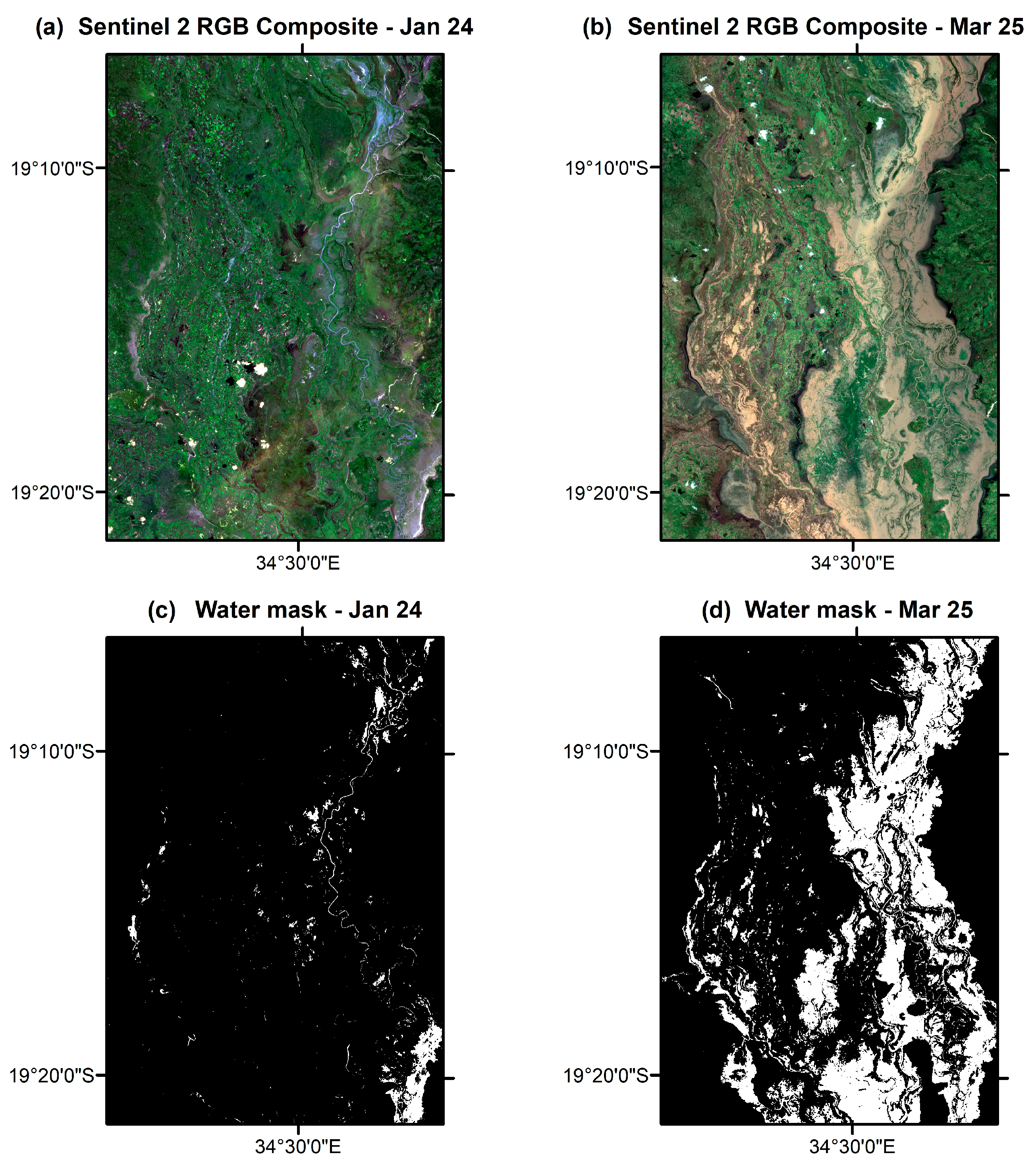
Binary flood maps from the automatic thresholding and probabilistic approach were validated using S2 optical imagery (Figure 2) from the same date, as this was the best available dataset in absence of in situ data. The Modified Normalized Difference Water Index (MNDWI) [52] was used to detect water bodies in the pre-event and during-flood images:
where is the reflectance from green band, and is the one from shortwave infrared. Next, the Otsu method was again utilized to identify a suitable threshold to classify water features [53]. The water bodies extents for the two epochs were then compared, thus obtaining the extent of the inundated zones. Accuracy metrics such as overall accuracy (OA), producer accuracy (PA), user’s accuracy (UA), and Cohen’s Kappa were then calculated for each dataset. Additionally, the Area Under the Receiver Operating Characteristic Curve (AUC) was computed in order to assess the performance of the SNDSI flood probabilistic raster.
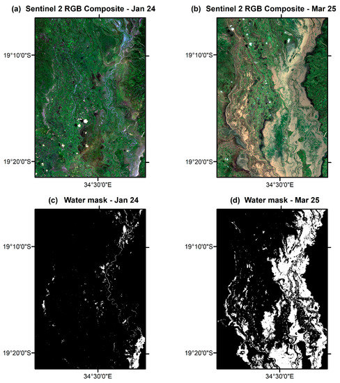
Figure 2.
Sentinel 2 RGB imagery and their respective water mask for pre-event (a,c) and during-event (b,d). The water mask was derived from Modified Normalized Difference Water Index (MNDWI) and Otsu thresholding.
5. Results
5.1. NDSI Thresholding
The results from AOI 1 and 2 show that open water flooding is easily detected in the NDSI product. As seen in Figure 3a, inundated zones exhibit very low negative NDSI values (lower than −0.6, shown in deep blue color) as a result of a dramatic decrease of backscattering intensity due to the mirror-like properties of the water surface. Moreover, the histograms of the cross and co-polarized products exhibit the same pattern: a bimodal distribution with one of the peaks centered near the lower limit of the distribution, and the other centered around zero.
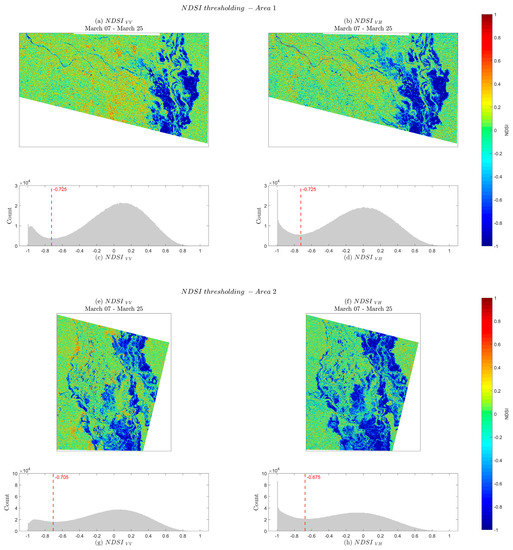
Figure 3.
Normalized Difference Sigma-Naught Index (NDSI) for Vertical Transmit-Vertical Receive (VV) and Vertical Transmit-Horizontal Receive (VH) polarization and their respective histograms for Area 1 (a,b,c,d) and Area 2 (e,f,g,h).
From the histogram, it can be inferred that two different populations are present in the data and that a threshold can be used to separate them. For Area 1, our described automated method set the threshold at −0.725, regardless of the polarization.
Similarly, the results for AOI 2 are congruent with those obtained in Area 1. Pixels potentially covered by water are those that present the lowest NDSI value, and given the magnitude of the flooding extent for this area, there is a large bin count for NDSI less than −0.6 in the two histograms (Figure 3b). The NDSI thresholds for VV and VH products were found at −0.705 and −0.675, respectively.
5.2. SNDSI Thresholding
The Shannon’s entropy of NDSI for both AOI is shown in Figure 4. At first sight, it is visible that inundated pixels correspond to the areas where the randomness (entropy) is closer to zero. Very low entropy indicates that the texture is similar within the inundated plains. Since a flooded pixel is usually surrounded by other flooded pixels, except in the boundaries of flooded and non-flooded areas, a very low entropy is obtained since many of the pixels within the moving window have very similar values.
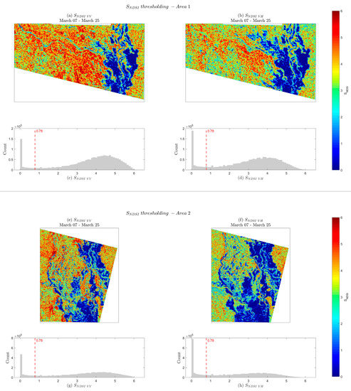
Figure 4.
Shannon’s entropy of NDSI (SNDSI) for VV and VH polarization and their respective histograms for Area 1 (a,b,c,d) and Area 2 (e,f,g,h).
Visual inspection of the four SNDSI results reveals that the spatial extent of the flooding is larger for the cross-polarized dataset. Additionally, the calculated classification threshold did not vary for any of the datasets (SNDSI = 0.78).
5.3. Accuracy Assessment
In general terms, the accuracy obtained by the first valley automatic thresholding method produced good results, as the validation with S2 data reveals in Table 2.

Table 2.
Estimated flooded area and accuracy assessment for automatic thresholding method.
Firstly, the NDSI thresholding for both AOI yielded results with PA ranging from 45% to 72%, with Cohen’s Kappa within the 0.51–0.68 range. The overall accuracy obtained with the NDSI is higher than 85% in all cases. When the performance between VV and VH polarization is compared, it can be seen that cross-polarization had lower omission errors (i.e., higher producer’s accuracy) than the co-polarization dataset.
Next, the SNDSI results show even higher accuracy results, with Kappa of 0.70–0.77 and OA ranging from 90% to 94%. In almost all cases, the omission and commission errors are considerably reduced when the entropy filter was applied to NDSI prior to the thresholding. In addition, cross-polarization also works better in both AOI, indicating that whether it is with NDSI or SNDSI, better results can be obtained with VH polarization.
The reference total flood extents estimated from optical imagery were 25.03 and 88.02 km2 for AOI 1 and AOI 2, respectively. Table 2 shows that VV polarization tends to yield lower flood extents when compared to VH polarization. Furthermore, Shannon’s entropy of NDSI in VH polarization produces flood estimates higher than the reference optical data. The results indicate the detectability of the roughness change of the land surface is different between VV and VH polarization. It can be hypothesized that the VV backscatter response is more sensitive to the wind roughening of the water surface [53]. However, to explore the detail sensing mechanism in the study area requires further analysis.
The results obtained from the automatic thresholding method are comparable to previous studies that utilized Sentinel 1 imagery for flood mapping. Cian et al. [33] generated flood maps for the flooding events in Malawi, Africa (2015) with an overall accuracy of 96.7%. Similar results were obtained by Clement et al. [53] when mapping flooding in Yorkshire, UK in 2015–2016 using the Change Detection and Threshold (CDAT) methodology, obtaining maps with total accuracy of 97%.
5.4. Bayesian Probabilistic Flood Mapping with SNDSI
The combination of the Weibull and Gaussian PDFs was capable of adequately describing the distribution of the flooded and non-flooded groups in the SNDSI images, as seen in Figure 5. The peak of each analyzed histogram is found in the lowest entropic states, decaying towards higher entropy values until another local peak is reached around the center of the distribution. Moreover, the R2 for all the four curve fitting models was between 0.95–0.98.
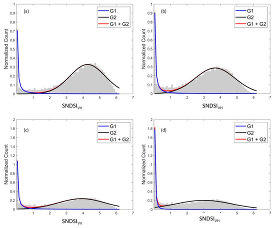
Figure 5.
Histogram curve fitting for SNDSI in VV and VH polarization for AOI 1 (a,b) and AIO 2 (c,d).
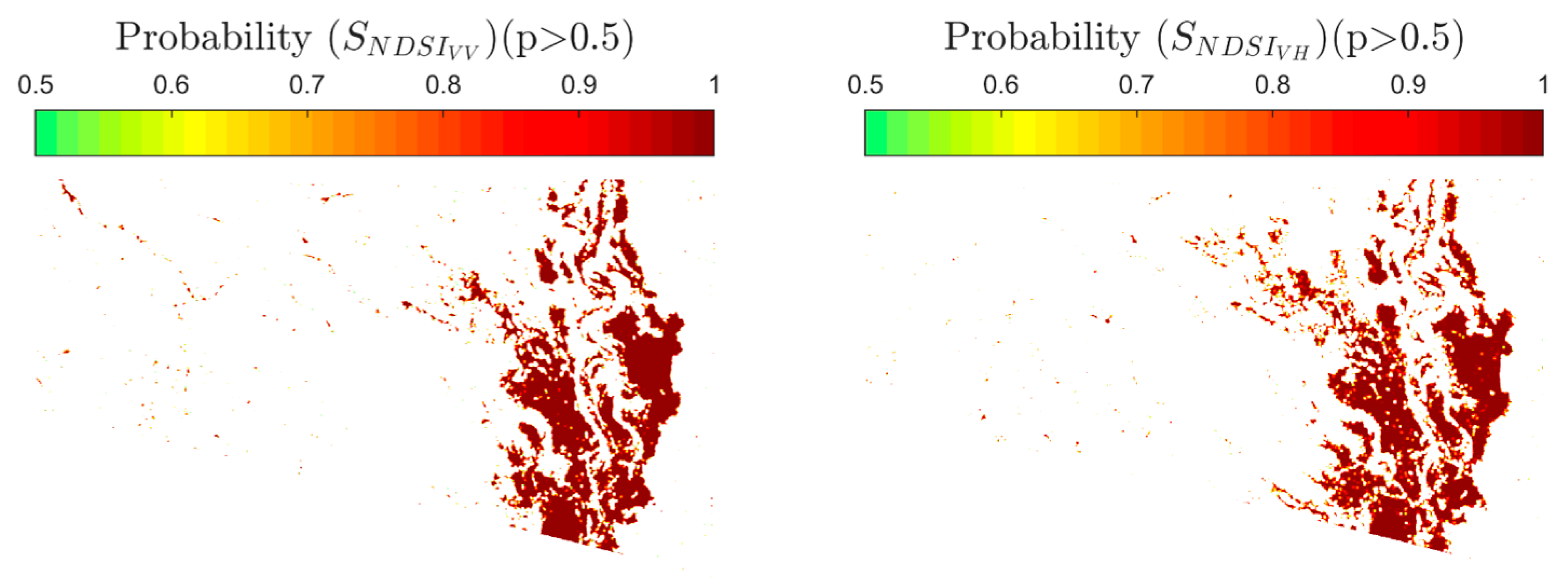
The histogram curve-fitting allows us to derive the required parameters to calculate the probability of a pixel of being flooded given a SNDSI value in the Bayesian framework, using Equation (3). As a result, a flood probability map was obtained, with values ranging from 0 to 1. We selected a cutoff threshold of p > 0.5 to separate flooding and non-flooding categories. The resulting flood probability maps for AOI 1 and 2 in VV and VH polarizations are shown in Figure 6 and Figure 7.
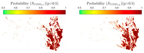
Figure 6.
Flood probability map for AOI 1 in VV (left) and VH (right) polarizations.
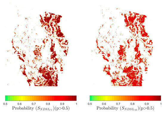
Figure 7.
Flood probability map for AOI 2 in VV (left) and VH (right) polarizations.
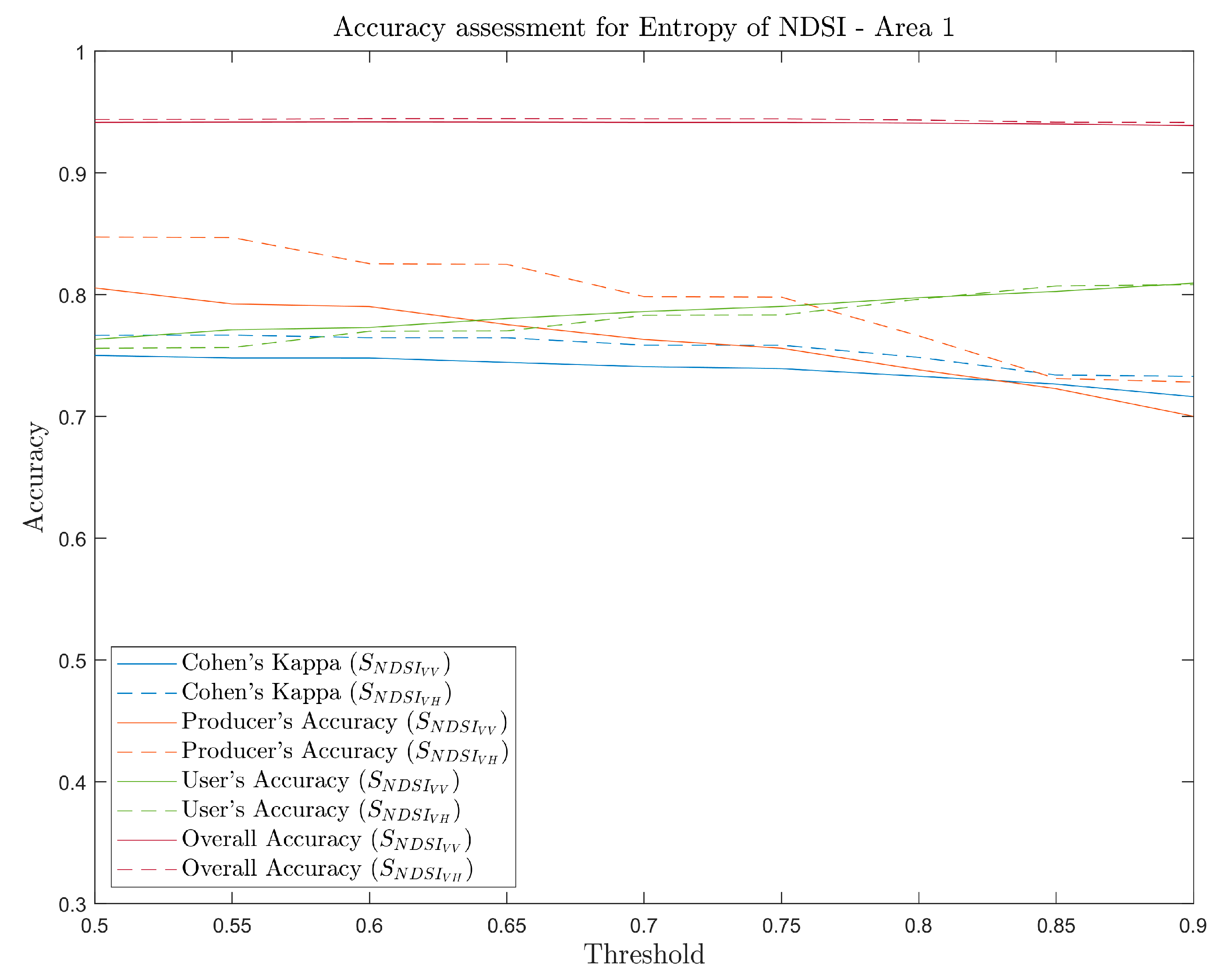
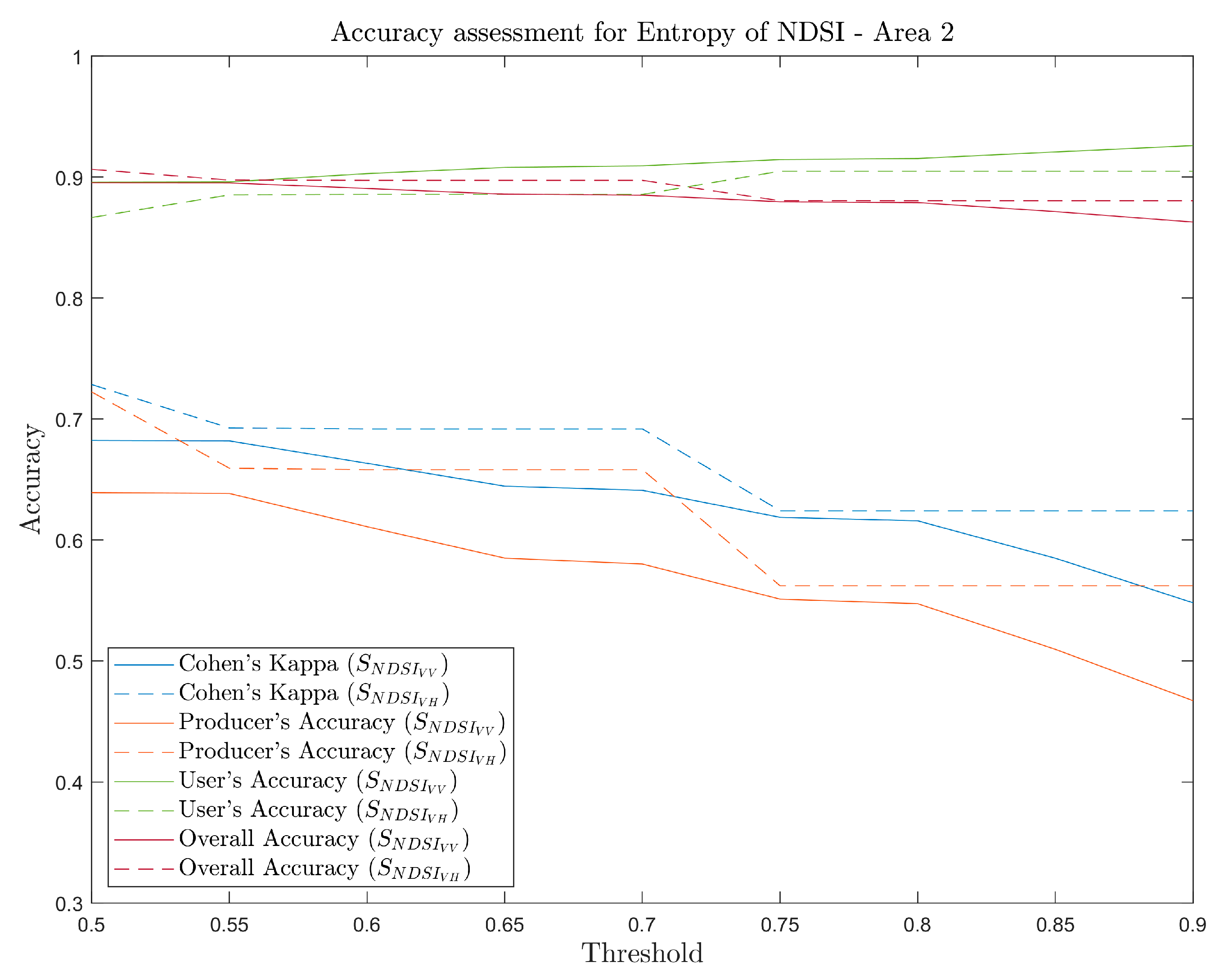
The pixels with the highest flooding probability exhibit a spatial pattern similar to the results of our automatic threshold method. The flood extents calculated for AOI 1 and AOI 2 are 26.82 and 74.72 km2 for VV polarization, and 29.06 and 86.97 km2 in VH polarization. Since the output of the Bayesian approach is a continuous raster, we examined the performance of the accuracy parameters at different probability levels, as shown in Figure 8.
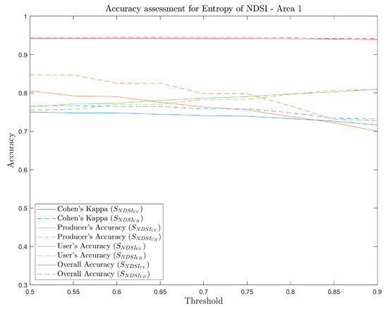
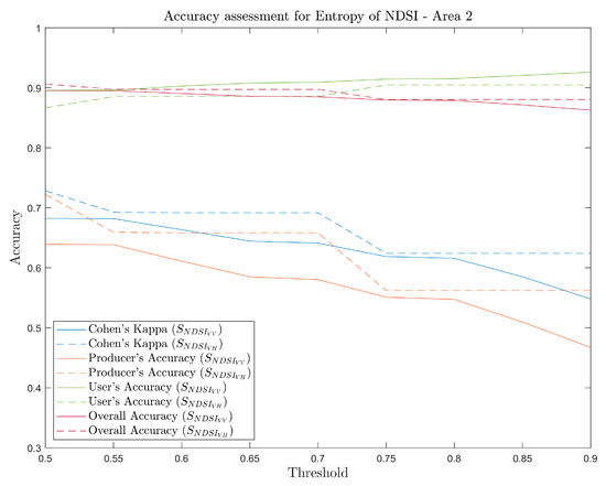
Figure 8.
Accuracy performance of NSDI in AOI 1 (up) and AOI 2 (down) at different probability intervals.
The Bayesian approach using texture information of the normalized backscattering difference produces results with good accuracy even at very conservative probability values. For AOI 1, the results indicate that the performance is quite stable from p > 0.5 to p > 0.9, indicating that the confidence level for flooded pixels is strong. On the other hand, in the case of AOI 2, Kappa higher than 0.65 was obtained when applying more relaxed thresholds, but we also noticed a drop in the accuracy metrics value as the probability cutoff increased, observing a considerable decline at p > 0.7. Additionally, as in the threshold classification, the accuracy of the classification is higher when VH polarization was used, thanks to better detection of true positive flooding pixels.
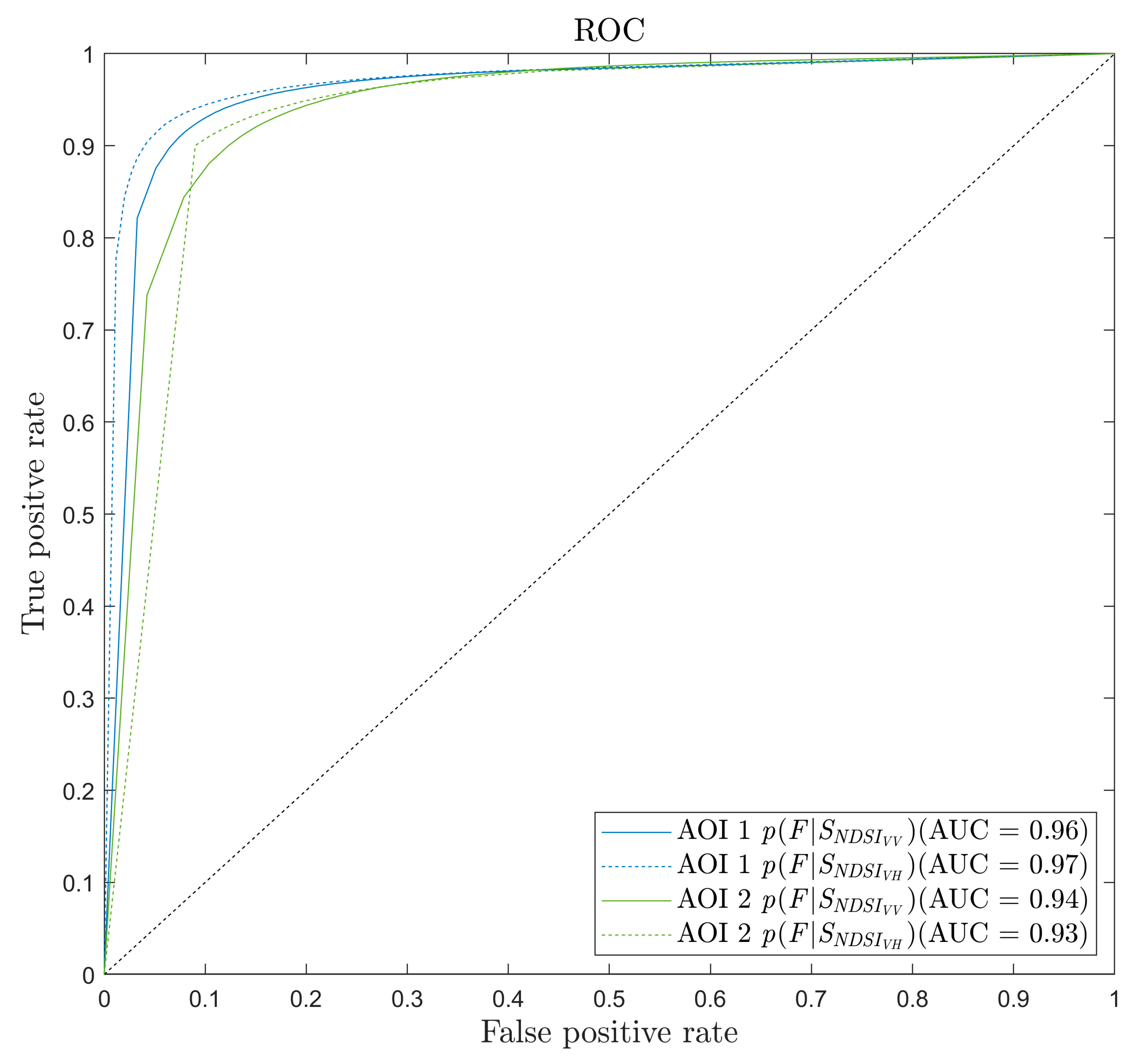
Further analysis was carried out by plotting the False Positive Rate (FPR) versus the sensitivity at different thresholds settings (Figure 9). The AUC values reported in Figure 9 show that our Bayesian model is capable of distinguishing between the two classes of interest: flooded and non-flooded. The two AUC values of AOI 1 are 0.96 (VV) and 0.97 (VH), respectively, indicating a very satisfied classifier, whereas a value of 0.5 indicates a completely random detector. For AOI 2, the AUC is 0.94 for the co-polarized model, and 0.93 for the cross-polarized.
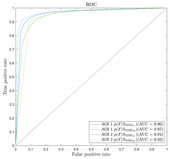
Figure 9.
Area Under the Receiver Operating Characteristic Curve (AUC) for flood probability map in both AOI.
6. Discussion
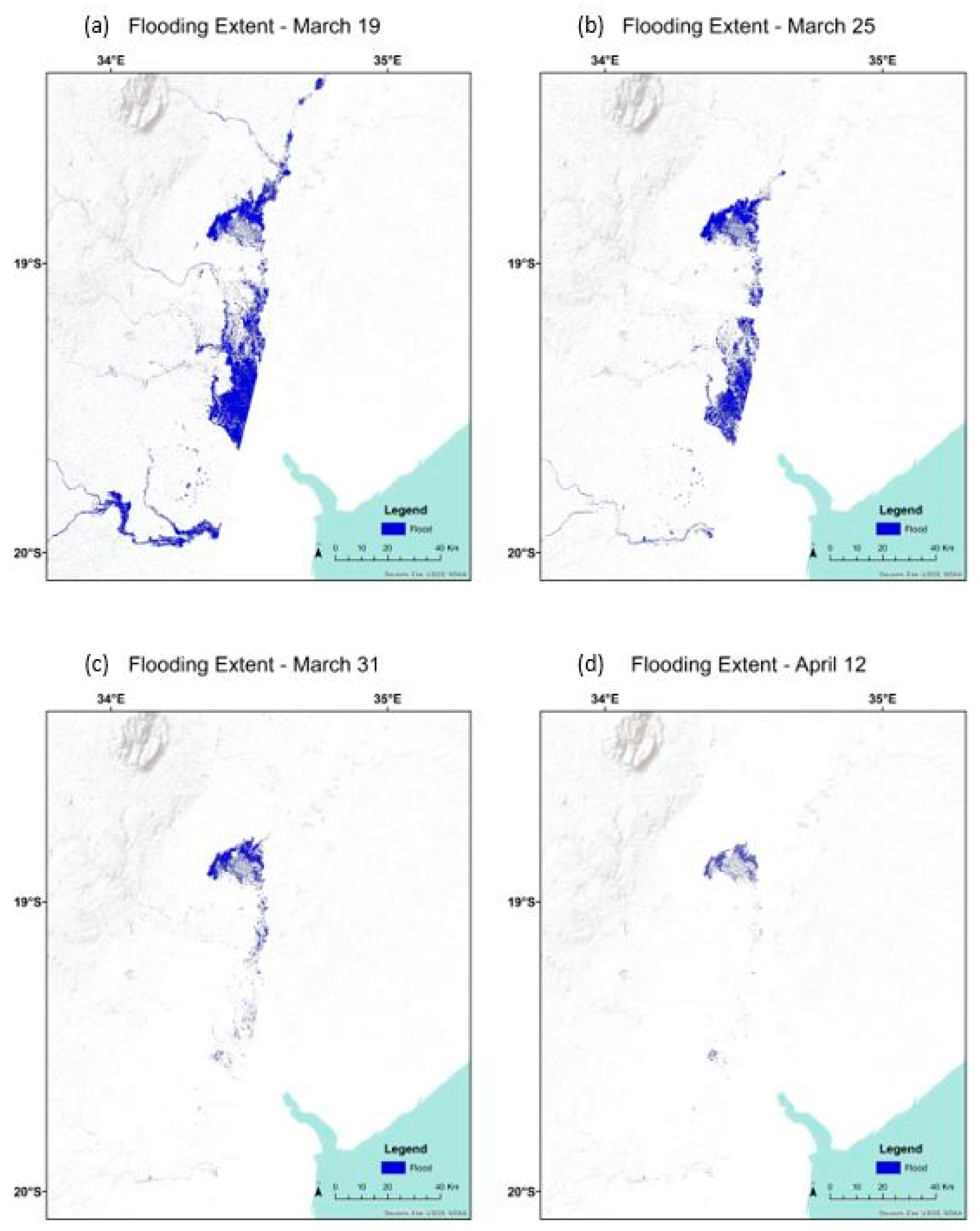
The effectiveness and minimal processing time of this proposed methodology makes it possible to produce flood proxy maps as soon as a new SAR scene is available. This is beneficial in situations such as emergency response scenarios, where time is a crucial asset and estimations of affected areas are necessary as soon as new data is ingested. To showcase its potential, we produced a Flood Proxy Map (FPM) time series for the Cyclone Idai, using the NDSI with VH polarization. The calculated thresholds were applied to the whole S1 scene. The during-flooding images correspond to the dates 19, 25, 31 March, and 12 April.
As seen in Figure 10, the largest extent of the flooded area was detected five days after the landfall of the Cyclone, on 19 March. The subsequent FPM reveal that a significant portion of the Sofala province was still inundated when the second post-event scene was acquired on 25 March. Six days later, the flooding receded significantly in the south section of the site. Finally, by 12 April, mostly areas nearby Lake Urema are identified as potentially flooded zones.
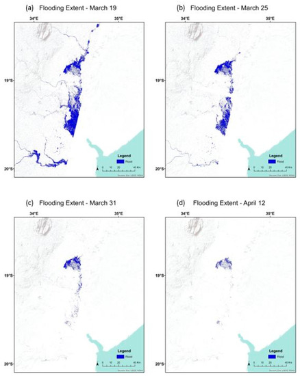
Figure 10.
Flood Proxy Maps time series (19 March (a), 25 March (b), 31 March (c), and 12 April (d)) for Cyclone Idai in Mozambique using automatic thresholding on S1 NDSI VH.
Furthermore, the usage of texture information in the form of an entropy filter of the NDSI enhances the accuracy of the proposed method. This approach presents a clear benefit: the texture of the SAR target and the spatial correlation between SAR pixels are both taken into account. By combining these two additional characteristics in a single product, we are able to improve the accuracy of open water flood proxy mapping over a large geographical region. In addition, our novel combination of Weibull and Gaussian PDFs allowed for the derivation of a continuous probability flood proxy map. Although the accuracy metrics are slightly lower than those obtained in the thresholding method, a continuous probabilistic product has the advantage over a binary map in that the former can provide the information of uncertainty associated with the classification.
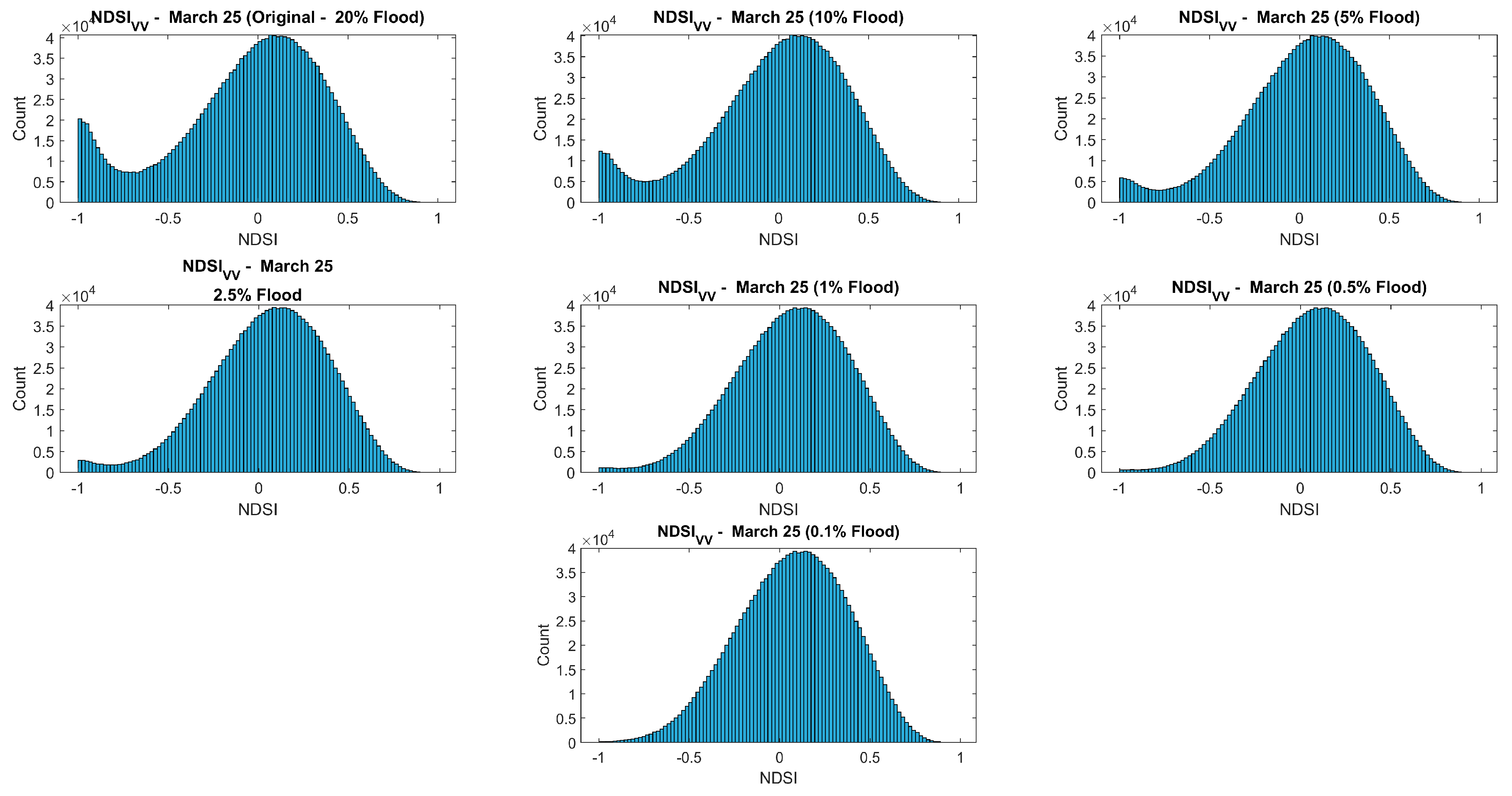
Nonetheless, some factors can influence the performance of the models presented, which merit further research and should be considered when applying these methods to other study areas. Firstly, the selection of an appropriate AOI is essential for the proper description of the flooded and non-flooded categories. An adequate AOI is one that contains considerable samples of both classes so that the histogram can properly describe their distribution. To highlight this issue, an experiment was conducted to explore the effect of the flood vs. non-flood sample ratio on the proposed method, by changing the ratio of flooded coverage of an AOI. The NDSI VV polarization data of AOI 1 (25 March 2019) was used to perform the test. Specifically, we randomly excluded flooded pixels from AOI 1 while maintaining the number of non-flooded pixels constant to simulate various flooded coverages: 20%, 10%, 5%, 2.5%, 1%, 0.5%, and 0.1% of the total area (Figure 11).
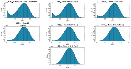
Figure 11.
Simulated NDSI histograms (VV polarization, March 25, 2019) with flooded coverages of 20%, 10%, 5%, 2.5%, 1%, 0.5% and 0.1% of the total area.
In Figure 11, the flooded area in the original AOI 1 is about 20% of the total area. As this percentage decreases, the left tail of the histogram becomes less prominent. Once the flooded area percentage reaches 0.5% and below, no threshold can be detected. This shows a limitation of this proposed approach: if the flooding is very small compared to the size of the clipped area, no threshold will be estimated.
Secondly, it is important to highlight that Shannon’s entropy, as a measure of texture in an image, is scale-dependent. The selection of the moving window size should be done according to the target of interest, but it is worth keeping in mind that smaller window sizes result in raster with a limited range of possible values, and when the histogram is computed it resembles a discretely sampled signal, with the bins very apart from one another. If the number of bins is not large enough, the curve fitting of the histogram may incur larger errors, or no converge at all.
Additionally, the land cover types present in any potential AOI could also affect the performance of this proposed method. Analysis of the land cover types for both Areas of Interest using the Copernicus Global Land Cover Layers [27] dataset reveals that in AOI 1 there are two predominant types of land cover classes: open forest and closed deciduous needle leaf forest, making up 60% of the study site. On the other hand, AOI 2 exhibits a more heterogeneous landscape, with only one predominant land cover class (open forest). The applicability of this approach is yet to be explored in urban environments, where the density of tall buildings could decrease the accuracy of the flood maps.
Another factor to take into account is the reduction in contrast between flooded and non-flooded areas as a consequence of wind-induced water surface roughness. Strong-wind conditions can affect the scattering mechanisms of open-water flooding sites, reducing its specular characteristics [54]. As a result, the normalized difference of the backscattering between the pre-flood and during-flood epochs might be lower. The impact that wind speed and direction have over the scattering mechanism of co-polarized and cross-polarized radar signals on open-water flooded surfaces is yet to be explored.
Finally, the detection of flooded areas with this method can be further improved by including topographical information into the workflow. Terrain filters such as slope and Height Above Drainage [55] can be incorporated to exclude areas where flooding is not possible, such as terrains with a steep slope or located too high above the nearest drainage line [56,57]. The magnitude at which the false positives are reduced thanks to the terrain filter will depend on the topographic conditions of the study site.
7. Conclusions
In this study, we demonstrate the applicability of the Normalized Difference Sigma-Naught Index for flood proxy mapping using an automatic threshold detection approach, as well as using the texture information of the image for estimating per-pixel flood probability. When using this proposed method to detect open water flooding over Mozambique after the landfall of cyclone Idai, we were able to obtain results with high accuracy, with Overall Accuracy between 85% and 93% and Kappa within the range 0.51–0.77. Moreover, the implementation of a moving window to calculate the randomness in the images reduces salt-and-pepper noise and decreases the omission errors for the flooded category.
We also found that Weibull distribution is suitable to describe rapidly decaying states, such as the low entropy populations in the SNDSI image. In this study, flooded zones are found to have similar texture characteristics that yield very low entropy zones. By using a Weibull PDF during the histogram curve-fitting process, we were able to properly describe the distribution of the inundated population within the normalized difference scattering data. The generated flood probability map was found to correctly identify the target class with Kappa > 0.65 for most confidence level thresholds, and its ROC yield AUC values between 0.93–0.97. This indicates that accurate flood mapping can be achieved with the proposed method. However, some limitations should be noticed in advance when the method is applied. First, the flood vs. non-flood sample ratio can affect the automatic thresholding procedure. Our experiment shows that flooded pixels could be misclassified when the flooded area percentage of the analyzed AOI is lower than 0.5%. Second, strong-wind conditions during Sentinel-1 image acquisition could have a strong impact on the validity of the mapping result. Nevertheless, thanks to its low computational cost, we suggest the proposed method has great potential to be applied in an emergency response situation for near-real-time monitoring of flooding events.
Author Contributions
Conceptualization, S.-H.C. and N.I.U.; methodology, S.-H.C. and N.I.U.; writing—original draft preparation, S.-H.C. and N.I.U.; writing—review and editing, S.-H.C., N.I.U., and S.-H.Y.; supervision, S.-H.C. and S.-H.Y.; funding acquisition, S.-H.C. All authors have read and agreed to the published version of the manuscript.
Funding
This research was funded by Taiwan’s Ministry of Science and Technology (MOST 108-2621-M-008-002-) and Hakka Affairs Council (HAC-108-IP-0005-01-04).
Acknowledgments
Part of the research was carried out at the Jet Propulsion Laboratory, California Institute of Technology, under a contract with the National Aeronautics and Space Administration (NASA Program NNH16ZDA001N-GEO). We would like to thank the editor and anonymous reviewers for providing constructive comments to improve the quality of this research.
Conflicts of Interest
The authors declare no conflict of interest.
References
- Jha, M.K. Natural and Anthropogenic Disasters: Vulnerability, Preparedness and Mitigation; Springer: Dordrecht, The Netherlands, 2010. [Google Scholar]
- Keller, E.; DeVecchio, D. Natural Hazards—Earth’s Processes as Hazards, Disasters, and Catastrophes, 5th ed.; Routledge: New York, NY, USA, 2019; p. 632. [Google Scholar]
- Organization for Economic Cooperation and Development. Financial Management of Flood Risk; OECD: Paris, France, 2016. [Google Scholar]
- Sen, Z. Flood Modeling, Prediction and Mitigation; Springer: Cham, Switzerland, 2018; p. 422. [Google Scholar]
- Bohorquez, P.; del Moral-Erencia, D.J. 100 Years of Competition between Reduction in Channel Capacity and Streamflow during Floods in the Guadalquivir River (Southern Spain). Remote Sens. 2017, 9, 727. [Google Scholar] [CrossRef]
- Tong, X.; Luo, X.; Liu, S.; Xie, H.; Chao, W.; Liu, S.; Makhinov, A.; Makhinova, A.; Jiang, Y. An approach for flood monitoring by the combined use of Landsat 8 optical imagery and COSMO-SkyMed radar imagery. ISPRS J. Photogramm. Remote Sens. 2018, 136, 144–153. [Google Scholar] [CrossRef]
- Sukojo, B.M.; Alfiansyah, F. Flood Disaster Analysis Using Landsat-8 and SPOT-6 Imagery for Determination of Flooded Areas in Sampang, Madura. IOP Conf. Ser. Earth Environ. Sci. 2017, 98, 012021. [Google Scholar] [CrossRef]
- Goffi, A.; Stroppiana, D.; Brivio, P.A.; Bordogna, G.; Boschetti, M. Towards an automated approach to map flooded areas from Sentinel-2 MSI data and soft integration of water spectral features. Int. J. Appl. Earth Obs. Geoinf. 2020, 84, 101951. [Google Scholar] [CrossRef]
- Refice, A.; D’Addabbo, A.; Capolongo, D. Flood Monitoring through Remote Sensing; Springer: Cham, Switzerland, 2018; p. 209. [Google Scholar]
- Schumann, G.; Bates, P.D.; Apel, H.; Aronica, G.T. Global Flood Hazard Mapping, Modeling, and Forecasting; Global Flood Hazard; American Geophysical Union: Washington, DC, USA, 2018; pp. 239–244. [Google Scholar]
- Schumann, G.J.P.; Moller, D.K. Microwave remote sensing of flood inundation. Phys. Chem. Earth Parts A/B/C 2015, 83–84, 84–95. [Google Scholar] [CrossRef]
- White, L.; Brisco, B.; Dabboor, M.; Schmitt, A.; Pratt, A. A Collection of SAR Methodologies for Monitoring Wetlands. Remote Sens. 2015, 7, 7615–7645. [Google Scholar] [CrossRef]
- Ndikumana, E.; Ho Tong Minh, D.; Baghdadi, N.; Courault, D.; Hossard, L. Deep Recurrent Neural Network for Agricultural Classification using multitemporal SAR Sentinel-1 for Camargue, France. Remote Sens. 2018, 10, 1217. [Google Scholar] [CrossRef]
- Townsend, P. Mapping Seasonal Flooding in Forested Wetlands Using Multi-Temporal Radarsat SAR. Photogramm. Eng. Remote Sens. 2001, 67, 857–864. [Google Scholar]
- Oberstadler, R.; Honsch, H.; Huth, D. Assessment of the mapping capabilities of ERS-1 SAR data for flood mapping: A case study in Germany. Hydrol. Process. 1997, 11, 1415–1425. [Google Scholar] [CrossRef]
- Pulvirenti, L.; Chini, M.; Pierdicca, N.; Boni, G. Use of SAR Data for Detecting Floodwater in Urban and Agricultural Areas: The Role of the Interferometric Coherence. IEEE Trans. Geosci. Remote Sens. 2016, 54, 1532–1544. [Google Scholar] [CrossRef]
- Martinis, S.; Kersten, J.; Twele, A. A fully automated TerraSAR-X based flood service. ISPRS J. Photogramm. Remote Sens. 2015, 104, 203–212. [Google Scholar] [CrossRef]
- Twele, A.; Cao, W.; Plank, S.; Martinis, S. Sentinel-1-based flood mapping: A fully automated processing chain. Int. J. Remote Sens. 2016, 37, 2990–3004. [Google Scholar] [CrossRef]
- Schumann, G.; Henry, J.; Hoffmann, L.; Pfister, L.; Pappenberger, F.; Matgen, P. Demonstrating the high potential of remote sensing in hydraulic modelling and flood risk management. In Proceedings of the Annual Conference of the Remote Sensing and Photogrammetry Society with the NERC Earth Observation Conference, Portsmouth, UK, 6–9 September 2005. [Google Scholar]
- Brown, K.M.; Hambidge, C.H.; Brownett, J.M. Progress in operational flood mapping using satellite synthetic aperture radar (SAR) and airborne light detection and ranging (LiDAR) data. Prog. Phys. Geogr. Earth Environ. 2016, 40, 196–214. [Google Scholar] [CrossRef]
- Brivio, P.A.; Colombo, R.; Maggi, M.; Tomasoni, R. Integration of remote sensing data and GIS for accurate mapping of flooded areas. Int. J. Remote Sens. 2002, 23, 429–441. [Google Scholar] [CrossRef]
- Henry, J.B.; Chastanet, P.; Fellah, K.; Desnos, Y.L. Envisat multi-polarized ASAR data for flood mapping. Int. J. Remote Sens. 2006, 27, 1921–1929. [Google Scholar] [CrossRef]
- Zoka, M.; Psomiadis, E.; Dercas, N. The Complementary Use of Optical and SAR Data in Monitoring Flood Events and Their Effects. Proceedings 2018, 2, 644. [Google Scholar] [CrossRef]
- The Earth Observatory. Devastation in Mozambique. 2019. Available online: https://earthobservatory.nasa.gov/images/144712/devastation-in-mozambique (accessed on 11 December 2019).
- Probst, P.; Annunziato, A. Tropical Cyclone IDAI: Analysis of the Wind, Rainfall and Storm Surge Impact; European Comission Joint Research Centre: Iapra, Italy, 2019. [Google Scholar]
- Global Facility for Disaster Reduction and Recovery. Mozambique Cyclone Idai Post-Disaster Needs Assessment; Global Facility for Disaster Reduction and Recovery: Washington, DC, USA, 2019. [Google Scholar]
- Buchhorn, M.; Lesiv, M.; Tsendbazar, N.E.; Herold, M.; Bertels, L.; Smets, B. Copernicus Global Land Cover Layers—Collection 2. Remote Sens. 2020, 12, 1044. [Google Scholar] [CrossRef]
- Schubert, A.; Miranda, N.; Geudtner, D.; Small, D. Sentinel-1A/B Combined Product Geolocation Accuracy. Remote Sens. 2017, 9, 607. [Google Scholar] [CrossRef]
- Torres, R.; Snoeij, P.; Geudtner, D.; Bibby, D.; Davidson, M.; Attema, E.; Potin, P.; Rommen, B.; Floury, N.; Brown, M.; et al. GMES Sentinel-1 mission. Remote Sens. Environ. 2012, 120, 9–24. [Google Scholar] [CrossRef]
- Tamm, T.; Zalite, K.; Voormansik, K.; Talgre, L. Relating Sentinel-1 Interferometric Coherence to Mowing Events on Grasslands. Remote Sens. 2016, 8, 802. [Google Scholar] [CrossRef]
- Schubert, A.; Small, D.; Miranda, N.; Geudtner, D.; Meier, E. Sentinel-1A Product Geolocation Accuracy: Commissioning Phase Results. Remote Sens. 2015, 7, 9431–9449. [Google Scholar] [CrossRef]
- Gorelick, N.; Hancher, M.; Dixon, M.; Ilyushchenko, S.; Thau, D.; Moore, R. Google Earth Engine: Planetary-scale geospatial analysis for everyone. Remote Sens. Environ. 2017, 202, 18–27. [Google Scholar] [CrossRef]
- Cian, F.; Marconcini, M.; Ceccato, P. Normalized Difference Flood Index for rapid flood mapping: Taking advantage of EO big data. Remote Sens. Environ. 2018, 209, 712–730. [Google Scholar] [CrossRef]
- Sovdat, B.; Kadunc, M.; Batič, M.; Milčinski, G. Natural color representation of Sentinel-2 data. Remote Sens. Environ. 2019, 225, 392–402. [Google Scholar] [CrossRef]
- Rapinel, S.; Mony, C.; Lecoq, L.; Clément, B.; Thomas, A.; Hubert-Moy, L. Evaluation of Sentinel-2 time-series for mapping floodplain grassland plant communities. Remote Sens. Environ. 2019, 223, 115–129. [Google Scholar] [CrossRef]
- Drusch, M.; Del Bello, U.; Carlier, S.; Colin, O.; Fernandez, V.; Gascon, F.; Hoersch, B.; Isola, C.; Laberinti, P.; Martimort, P.; et al. Sentinel-2: ESA’s Optical High-Resolution Mission for GMES Operational Services. Remote Sens. Environ. 2012, 120, 25–36. [Google Scholar] [CrossRef]
- Vuolo, F.; Żółtak, M.; Pipitone, C.; Zappa, L.; Wenng, H.; Immitzer, M.; Weiss, M.; Baret, F.; Atzberger, C. Data Service Platform for Sentinel-2 Surface Reflectance and Value-Added Products: System Use and Examples. Remote Sens. 2016, 8, 938. [Google Scholar] [CrossRef]
- Furuta, R.; Tomiyama, N. A Study of Detection of Landslide Disasters due to the Pakistan Earthquake using ALOS data. In Proceedings of the 34th International Symposium on Remote Sensing of Environment, Sydney, Australia, 7 November 2011. [Google Scholar]
- Prieto-Guerrero, A.; Espinosa-Paredes, G. 7—Nonlinear signal processing methods: DR estimation and nonlinear stability indicators. In Linear and Non-Linear Stability Analysis in Boiling Water Reactors; Prieto-Guerrero, A., Espinosa-Paredes, G., Eds.; Woodhead Publishing: Cambridge, UK, 2019; pp. 315–398. [Google Scholar]
- Galar, D.; Kumar, U. Chapter 3—Preprocessing and Features. In eMaintenance; Galar, D., Kumar, U., Eds.; Academic Press: Cambridge, UK, 2017; pp. 129–177. [Google Scholar]
- Navarro, P.J.; Fernández-Isla, C.; Alcover, P.M.; Suardíaz, J. Defect Detection in Textures through the Use of Entropy as a Means for Automatically Selecting the Wavelet Decomposition Level. Sensors 2016, 16, 1178. [Google Scholar] [CrossRef]
- Gonzalez, R.C.; Woods, R.E. Digital Image Processing; Addison-Wesley Longman Publishing: Boston, MA, USA, 2001. [Google Scholar]
- Gonzalez, R.C.; Woods, R.E.; Eddins, S.L. Digital Image Processing Using MATLAB; Prentice-Hall: Upper Saddle River, NJ, USA, 2003. [Google Scholar]
- Giustarini, L.; Hostache, R.; Kavetski, D.; Chini, M.; Corato, G.; Schlaffer, S.; Matgen, P. Probabilistic Flood Mapping Using Synthetic Aperture Radar Data. IEEE Trans. Geosci. Remote Sens. 2016, 54, 6958–6969. [Google Scholar] [CrossRef]
- Lin, N.Y.; Yun, S.-H.; Bhardwaj, A.; Hill, M.E. Urban Flood Detection with Sentinel-1 Multi-Temporal Synthetic Aperture Radar (SAR) Observations in a Bayesian Framework: A Case Study for Hurricane Matthew. Remote Sens. 2019, 11, 1778. [Google Scholar] [CrossRef]
- Morton, J.C. Image Analysis, Classification and Change Detection in Remote Sensing: With Algorithms for Python, 4th ed.; CRC Press: Boca Raton, FL, USA, 2019. [Google Scholar]
- Westerhoff, R.S.; Kleuskens, M.P.H.; Winsemius, H.C.; Huizinga, H.J.; Brakenridge, G.R.; Bishop, C. Automated global water mapping based on wide-swath orbital synthetic-aperture radar. Hydrol. Earth Syst. Sci. 2013, 17, 651–663. [Google Scholar] [CrossRef]
- Yang, F.; Ren, H.; Hu, Z. Maximum Likelihood Estimation for Three-Parameter Weibull Distribution Using Evolutionary Strategy. Math. Probl. Eng. 2019, 2019, 1–8. [Google Scholar] [CrossRef]
- Le, T.M.; Fatahi, B.; Khabbaz, H.; Sun, W. Numerical optimization applying trust-region reflective least squares algorithm with constraints to optimize the non-linear creep parameters of soft soil. Appl. Math. Model. 2017, 41, 236–256. [Google Scholar] [CrossRef]
- Otsu, N. A Threshold Selection Method from Gray-Level Histograms. IEEE Trans. Syst. Man Cybern. 1979, 9, 62–66. [Google Scholar] [CrossRef]
- Chini, M.; Hostache, R.; Giustarini, L.; Matgen, P. A Hierarchical Split-Based Approach for Parametric Thresholding of SAR Images: Flood Inundation as a Test Case. IEEE Trans. Geosci. Remote Sens. 2017, 55, 6975–6988. [Google Scholar] [CrossRef]
- Xu, H. Modification of normalised difference water index (NDWI) to enhance open water features in remotely sensed imagery. Int. J. Remote Sens. 2006, 27, 3025–3033. [Google Scholar] [CrossRef]
- Clement, M.A.; Kilsby, C.G.; Moore, P. Multi-temporal synthetic aperture radar flood mapping using change detection. J. Flood Risk Manag. 2018, 11, 152–168. [Google Scholar] [CrossRef]
- Pierdicca, N.; Pulvirenti, L.; Chini, M. Flood Mapping in Vegetated and Urban Areas and Other Challenges: Models and Methods. In Flood Monitoring through Remote Sensing; Refice, A., D’Addabbo, A., Capolongo, D., Eds.; Springer International Publishing: Cham, Switzerland, 2018; pp. 135–179. [Google Scholar]
- Rennó, C.; Nobre, A.; Cuartas, L.; Soares, J.; Hodnett, M.; Tomasella, J.; Waterloo, M. HAND, a new terrain descriptor using SRTM-DEM: Mapping terra-firme rainforest environments in Amazonia. Remote Sens. Environ. 2008, 112, 3469–3481. [Google Scholar] [CrossRef]
- Bioresita, F.; Puissant, A.; Stumpf, A.; Malet, J.P. A Method for Automatic and Rapid Mapping of Water Surfaces from Sentinel-1 Imagery. Remote Sens. 2018, 10, 217. [Google Scholar] [CrossRef]
- Jafarzadegan, K.; Merwade, V. Probabilistic floodplain mapping using HAND-based statistical approach. Geomorphology 2019, 324, 48–61. [Google Scholar] [CrossRef]
© 2020 by the authors. Licensee MDPI, Basel, Switzerland. This article is an open access article distributed under the terms and conditions of the Creative Commons Attribution (CC BY) license (http://creativecommons.org/licenses/by/4.0/).

