Abstract
Synthetic Aperture Radar (SAR) Automatic Target Recognition (ATR), most algorithms of which have employed and relied on sufficient training samples to receive a strong discriminative classification model, has remained a challenging task in recent years, among which the challenge of SAR data acquisition and further insight into the intuitive features of SAR images are the main concerns. In this paper, a deep transferred multi-level feature fusion attention network with dual optimized loss, called a multi-level feature attention Synthetic Aperture Radar network (MFFA-SARNET), is proposed to settle the problem of small samples in SAR ATR tasks. Firstly, a multi-level feature attention (MFFA) network is established to learn more discriminative features from SAR images with a fusion method, followed by alleviating the impact of background features on images with the following attention module that focuses more on the target features. Secondly, a novel dual optimized loss is incorporated to further optimize the classification network, which enhances the robust and discriminative learning power of features. Thirdly, transfer learning is utilized to validate the variances and small-sample classification tasks. Extensive experiments conducted on a public database with three different configurations consistently demonstrate the effectiveness of our proposed network, and the significant improvements yielded to surpass those of the state-of-the-art methods under small-sample conditions.
1. Introduction
Since images from Synthetic Aperture Radar (SAR) Automatic Target Recognition (ATR) outperform optical images in their adaptivity to different weather, durability in time and extensity of detection range, SAR has always been a vital interest of numerous researchers of space-based earth observation. Automatic Target Recognition in SAR images, as a paramount means of assisting the manual interpretation of images and early warnings for national homeland security, plays an essential role in civil and military target perception in this field [1,2], primarily including reports of disaster information and prevention of natural disasters, identification and localization of military targets, etc. Although a great number of approaches have been developed for SAR ATR, which have attracted lots of attention [3,4] in the field, a multitude of limitations simultaneously are yet to be solved. The primary limitations of SAR ATR are insignificant image texture information, serious speckle noise, severe geometric distortion, critical structural defects, and low angle sensitivity.
Nowadays, the mainstream SAR automatic target recognition method can be generally classified into the template-oriented method and model-oriented method. The core of the template-oriented approach is feature extraction and selection depending on the foundation of deep domain knowledge theory. While the template-based SAR ATR method focuses on the construction of the feature library, the traditional feature extraction method with mainly handcrafted features is based on space, spectrum, texture, shape and other information. Typical features include texture description [5], gist [6], scale-invariant feature transform [7], gradient Histogram [8], local binary pattern [9], etc. The template-based approach with more outline features significantly reduces computational complexity. However, its limitation lies in the fact that some implicit key features cannot be effectively utilized, therefore considerably limiting or degrading the performance improvement, because the feature-based approach is an essentially sparse approach to feature space. The model-based approach, occupying model design as its core feature, mainly works on the construction of the physical model of the object, including its shape, geometry, texture, material and so on. The representation of the physical structure of the interest object is close to its physical essence, which shares the ability of better robustness and generality. Nevertheless, domain-related knowledge is a requisite for reducing the influence produced by the feature extraction and template-matching technology of SAR images, and yet the optimal classification feature of SAR images cannot be learned by the ATR system independently [10]. Many works have been concerned with SAR image classifications [11]. Clemente et al. [12] presented a method of military vehicles with Krawtchouk Moments to solve the SAR tasks and obtained a good performance in recognition. Sun et al. [13] proposed a dictionary learning and joint dynamic sparse representation method which is an effective way to recognize SAR images. Kim et al. [14] used Adaboost-based feature selection to robust ground target detection by SAR and IR sensor fusion to solve the background scatter noise problem and obtained excellent results. Thus, the traditional artificial image interpretation has an inferior efficiency, higher error rate, and more resource consumption, which cannot meet the needs of time-sensitive applications.
The deep learning method based on big data provides a new technical route without manual feature engineering and target modeling. Lin et al. [15] designed a unique architecture called the convolutional highway unit to extract deep feature representations for classification. Sharifzadeh et al. [16] applied a new hybrid Convolutional Neural Networks (CNN)-Multilayer Perceptron (MLP) classifier for ship classification in SAR images. Tian et al. [17] integrated a weighted kernel module (WKM) to improve the feature extraction capability into the commonplace CNN and achieved superior performance. Ma et al. [18] utilized a CNN-based method to work on ship classification and detection using GF-3 SAR images. Recent advances in CNNs have been widely borne out in various SAR targets, but SAR ATR still suffers from insufficient training samples and inferior optimized model design.
To our best knowledge, SAR target recognition depends on substantial labeled training images to train a robust model for classification, but is widely limited by space scope, region accessibility, and high-cost data acquisition. In this regard, this paper specifically serves to mitigate the dependence on large training samples by designing a network called a multi-level feature fusion attention network that combines the feature fusion method to attach more attention to the classification mechanism. For a better measure of quality on model predictions, a novel optimization method with batch normalization has been fashioned in this paper as well. Meanwhile, transfer learning is introduced to validate the optimized model by using pre-trained weights for a new classification.
The contributions are as follows:
1. MFFA-SARNET: A deep learning architecture exploiting a multi-level feature fusion scheme is utilized to refine the extracted features and subsequently discard background features learned from the SAR targets, considerably facilitating the function of weight distribution and task focus;
2. A dual optimized loss for training optimization: A dual optimized loss is composed of two losses, with one to encourage the interclass dissimilarity, and the other to serve as the constraint to balance network optimization, the combination of which has considerably ameliorated the discriminative power to accomplish the SAR classification task;
3. Transfer learning adaptation: the theory of transfer learning is utilized to enforce the feature representation in the case of small samples, which indicates that the performance of the proposed method surpasses those of other advance works;
4. Small-sample classification task: the proposed network validates its superiority in working with small samples under three different configurations, significantly reducing the data dependence and enabling insight into the raw images.
The remainder of the paper is organized as follows. Section 2 presents a brief introduction to the basic related work from previous researchers, while Section 3 expounds the notions of the proposed methods. After the analysis and results of the proposed methods are unveiled in Section 4, Section 5 draws a short conclusion of the whole paper.
2. Related Work
In recent years, the SAR ATR task has obtained quite a few preliminary results. Researchers often consider the extraction of robust features during feature extraction, whose methods according to mathematical transformation are widely applied in automatic target recognition for SAR images, containing linear feature extraction and nonlinear feature extraction. The data are analyzed and transformed by mathematical methods so that they can be better represented in the feature space by better discrimination features. The orthogonal transform such as K-L Transform, Hough Transform, Wavelet Transform, Radon transform, and Mellin transform [19,20], can be recruited to extract the orthogonal component of the target and reduce the correlation between the image pixels and the feature dimension of the feature space. In addition, in SAR ATR tasks, the main linear feature extraction methods include Principal Component Analysis (PCA) [21] and linear discriminant analysis (LDA) [22] based on the Fisher criterion. The results of both methods in the Moving and Stationary Target Acquisition and Recognition (MSTAR) database have verified the effectiveness of PCA and LDA in SAR image feature extraction.
Apart from the elements mentioned above, sparse representation theory has also attracted interest from a myriad of researchers, and has been deployed in numerous fields of image processing, such as dictionary learning, image denoising and so forth. For instance, Yang et al. initialed an efficient and reliable classification method called Sparse Representation Classification (SRC), which can construct an over-complete library used for the linear representation of testing samples. In [23], sparse representation is engaged in SAR target classification with 2D canonical correlation analysis, which gives satisfying results. Moreover, Yu et al. [24] propounded a method by a joint sparse and dense representation of the monogenic signal, greatly decreasing the complexity of the algorithm and enhancing the performance.
Thanks to the accessibility of adequate training samples and the introduction of Deep Neural Networks (DNN), it has become much more popular in the field of machine learning. Furthermore, it has been noticed that the multi-hidden layer artificial neural network (ANN) possesses the excellent ability of feature learning beneficial to visual classification [25]. Consequently, the training limitation of DNN can be solved by adopting the policy of layer-wise pre-training [26]. CNN, proposed by Lecun [27], is the first learning algorithm to train the multi-layer network successfully. It is capable of reducing the storage of learned parameters and improving the efficiency of the network by using the local connection and weight sharing of the network and backpropagation. With its outstanding edges, CNN was flexibly exercised in various works. Hinton et al. [28] applied CNN to ImageNet, the largest database for image recognition, with stunning results obtained, surpassing all the previous ones, while Zhang et al. [29] suggested an approach based on CNN cascaded features and an AdaBoost rotation forest to extenuate the problems arising from the lack of samples. In Liu et al. [30], the sparse manifold regularized networks were presented for polarimetric SAR terrain classification, in which the number of training samples was reduced by fine-tuning a few parameters.
Furthermore, as an important research direction in SAR ATR, multi-feature fusion cannot be ignored. In this area, Amrani et al. [31] deployed the traditional cascade and discriminant correlation analysis algorithm to fuse the extracted deep features while Wang et al. [32] proposed a two-channel feature fusion method for intensity features and gradient amplitude features. This representation method can effectively maintain the spatial relationship between the two features and achieve a better feature fusion effect. Zheng et al. [33] offered an improved form of CNN with higher generalization ability and less fitting probability, combining the convolution (conv) layer of CNN with a two-dimensional PCA algorithm to further improve its efficiency and robustness. Yu et al. [34] presented a deep feature fusion network acquiring prominent results under limited data conditions, on the basis of which a structure containing multi-input parallel network topology was created, where the SAR image features of different perspectives were extracted layer by layer, and the features of different viewpoints were merged step by step, which were robust to the change in the visual angle.
Transfer learning also plays an indispensable role in deep learning. In [35], transfer learning was introduced to transfer the prior experience learned from enough unmarked SAR images to marked SAR targets. Rostami et al. [36] trained a DNN for SAR targets by deep transferring the weights to the target task, successfully eliminating the need for sufficient samples. Xu et al. [37] employed framework-oriented transfer learning method with discriminative adaptation regularization for ship classification. In short, transfer learning can contribute to boosting performance in the case of a lack of training samples.
3. Proposed MFFA-SARNET
The proposed MFFA-SARNET scheme is explained in Figure 1 in meticulous detail. We will present our newly developed framework in this section. In our work, given the characteristics of SAR targets, SAR images are transferred into the proposed network, in which different level features from multiple layers are fused into the attention module to complete the weight distribution and task focus. After the framework has learned the attention area for the class to be identified, a novel loss function with batch normalization is applied to recognize the target, after which SAR targets transferred into the network are trained through the backpropagation algorithm. Data analysis displayed in Table 1 aims to augment data intuitiveness for an easier and better understanding from readers.
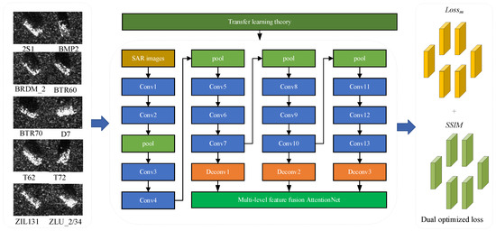
Figure 1.
The proposed multi-level feature fusion attention network with dual optimized loss. The diagram of the proposed classification framework can be divided into five parts. Feature Extractor 1 (Conv1–Deconv1), Feature Extractor 2 (Conv8–Deconv2), Feature Extractor 3 (Conv11–Deconv3), multi-level feature attention module and classifier which includes full connections 1 and 2 (fc1 and fc2). During the training stage, each feature extractor extracts feature information at different levels, such as shallow features, middle features, and high-level semantic features from raw images; then, all the learned features are concentrated to feature fusion before transferring into the attention module for task focus; finally, all the learned and attention features go through the classifier for the further classification task. During the training, the learned transferred parameters also serve in the network.

Table 1.
Data analysis of proposed multi-level feature attention Synthetic Aperture Radar network (MFFA-SARNET).
As displayed in Table 1, we could observe that parameters learned from each layer have been influenced by the network settings, from the parameters learned from the conv layers are increasing while descending after deconvolution (deconv) layers and fc1/fc2 layers. The final parameters are slightly smaller and are more effective for classification.
3.1. Multi-Level Feature Attention Network
3.1.1. Multi-Level Feature Extraction and Fusion
Feature fusion refers to the extraction of different types of features according to a method by utilizing a plurality of feature extraction methods. For its superiority in extracting abundant texture information and possessing promising robustness for various changes in images, it is well adapted to further mine image information. In this section, we optimized the accuracy of image recognition by adopting a method of multi-feature fusion, as shown in Figure 2. Specifically, SAR target classification is carried out by utilizing a method of multi-feature fusion, where SAR image classification is operated and assisted by the idea of low-level feature mapping and high-level semantic feature fusion with strong representation ability.
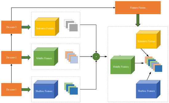
Figure 2.
Schematic diagram of the multi-level feature fusion process.
Suppose that the size of the feature map in convolution layers is (m×m)×n, with (m×m) as the feature map dimension, n as the network depth. The pixel region where the interaction between i-th mapping features and u×u×1 convolution kernel is , so the is formulated as follows:
where refers to the specific value of the i-th convolution kernel in the region (a, b). l denotes the l-th branch of the network. denotes the output feature map in the i-th layer from the branch l in the network. By using the function of weight , offset value and , the fusion feature mapping of the region is obtained:
where f is the affine transformation. This could be the activation functios for Rectified Linear Unit (ReLU), sigmoid, softmax, Exponential Linear Unit (ELU) and so on. The output feature maps can be described in another form, , among which j is one of the fusion branches, C denotes the channel number, and N stands for the number of training targets. [W, H], as the number of channels, appertains to the width and the height of the feature map, respectively. Assuming that the feature graph is calculated by Formula (2) and that tensor is a vector list containing the parameters N, C, W, H, the fusion procedure can be worked out as the process in Figure 2. In this paper, there are three branches named the o-th, p-th, and q-th branch, and the fusion feature in the branch o,p,q can be expressed as Formula (3):
The function of the multi-feature fusion module intends to obtain different feature graph information, to provide ample feature information for feature discrimination.
3.1.2. Attention Module
We investigated the attention mechanism, whose essence proves to locate the information of interest and suppress the useless information so that the SAR target’s features can be well focused. The results obtained from the former step are usually presented in the form of a probability graph or probability characteristic vector channel.
Figure 3 demonstrates the attention module containing the specific approach to channel attention, which can be illustrated as follows. Firstly, the feature tensor is transformed into U, where U = [u1, u2, …, uD], in which ui ∈ Rk represents the i-th dimension of the features, and D is the dimension of vi or the total number of channels in each domain. Then, we pool each channel to generate a channel vector shown in Formula (4).
where is the mean vector of , which denotes the feature of i-th channel. The process of the channel attention model is expressed as follows:
where Wvc, Wqc, and Wc are the embedding matrixes, while bvc, bqc and bc are the bias term. Q expresses the input vector of validation images. represents the outer product of a vector and the channel attention vector will be obtained through the channel attention mechanism Ac, which can be simplified as:
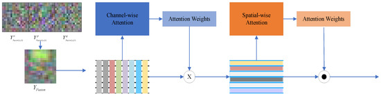
Figure 3.
Attention module.
Through the above steps from Formula (4)~(7), we can obtain the channel attention weight , thus feeding back to the channel attention function fc to calculate a feature map Vc.
where fc denotes the product of the channel and the corresponding channel weight of the region feature mapping at the channel level. V is the input feature map followed by the channel attention mechanism. Thus, the Vc can be represented as:
Given the calculated feature map Vc, new features are generated by inputting the Vc and Q into the network, and then the softmax function is employed to calculate the spatial attention weight based on the region. The spatial attention mechanism is defined as follows:
where and are the embedding matrices, mapping the visual and problem features to the shared latent space. Additionally, Wo is a set of parameters that needs to be relearned, b is a model bias term, and is a matrix and vector phase addition operation.
Simply, the attention weight can be optimized as:
3.2. The Dual Optimized Loss for Training Optimization
It is known that weaker classifiers should be used to improve the discriminative performance of the learned representations because the massive parameters may make the network prone to overfitting, especially for small samples. Besides, the cost function is also a perfect choice to improve performance by optimizing the network. To avoid overfitting and computation, network optimization also becomes one of the research hotspots. Chen et al. [38] proposed a new low-degree-of-freedom sparse connected convolution structure to replace the traditional full connection, which reduced the number of free parameters, optimized the serious over-fitting problem triggered by the limitation of the number of training images and adopted dropout technology, aiming to enhance the generalization ability. The small-batch random gradient drop method with momentum was used to optimize and quickly find the global optimum. Wilmanski et al. [39] were committed to the improvement of the learning algorithm, using AdaGrad and AdaDelta technology to avoid manually adjusting the learning rate and other parameters, engendering better robustness to parameter selection.
To optimize the classification of SAR images with noise-free tags, we designed a novel dual optimized loss with a batch normalization algorithm to gain an agreeable classification performance in this section. The loss function could be divided into two parts: Lossm and constraint SSIM. The former one is the modified softmax loss function with batch normalization. The depth feature of softmax training, which divided the entire hyperspace or hypersphere into categories based on the number of categories, ensuring that the categories were separable, proved ideal for multi-category tasks, under the condition that softmax did not require intra-class compactness and inter-class separation. For batch normalization, each batch was normalized to zero means, and the original data was mapped to a distribution with a mean of zero and a variance of one. The performance brought by BN contained the input distribution, which helpfully promoted the smoothness of the solution space of the optimization problem and the predictability and stability of the gradient. Therefore, we modified softmax with batch normalization, not only ensuring separability but also guaranteeing the best compactness of feature vector class and the greatest separation between classes.
If the input of the optimization part is xi, the batch normalization (BN) can be described as:
where refers to the mean value, the variance, the normalized value, and the batch normalization values, which is a posterior form of the Gaussian model with a pooled covariance matrix, serving to determine the prediction result.
The SSIM loss is a measure of the similarity between two images, to ensure and further improve the optimization, while it also serves as the constraint to balance network optimization. The SSIM defines the structure information irrelevant to brightness and contrast, to illustrate the object structure properties from the perspective of image composition.
The dual optimized loss is defined as follows:
where
where ys is the one-hot label, y is the output value, is the corresponding mean values, is the covariance between ys and y and C1 and C2 are the constants. To ensure a clearer understanding, Algorithm 1 demonstrates the training optimization in meticulous detail below.
Loss = log (Lossm) + β(1 − SSIM)
| Algorithm 1: Dual Optimized Loss for Training Optimization |
| Require: Constant C1, C2 |
| Require: The balanced parameter β |
| Require: Stepsize α |
| Require: β1, β2 ∈ [0,1): Exponential decay rates for the moment estimates |
| Require: θ0: Initial parameter vector |
| m0←0; |
| v0←0; |
| Given that the training set includes m samples in small batches, X = {x1, x2,…, xi}, the corresponding ground truth to the target is yi, and the corresponding output is ys |
| while θt is not converged, do: |
| Step 1: t ← t+1 |
| Step 2: Compute the mean ys and mean y: |
| Step 3: Compute the covariance y and ys: |
| Step 4: Simulate the value of Lossm and SSIM by Equation (15) |
| Step 5: Simulate the whole Loss by Equation (14) |
| Step 6: Loss optimization gained as follows |
| end while |
| return θt |
3.3. Transfer Learning
Transfer learning devotes itself to figuring out the shared characteristic between several tasks and transferring the weights at the level of general features. By training other image datasets like ImageNet, or learning other similar images from SAR images, the shallow, middle and high-level features that can be used to deal with classification tasks can be obtained, and leveraging data from related tasks can effectively improve generalization and reduce the runtime of evaluating a set of classifiers. The domain is described as D = {F, P(X)}, while F = {f1, f2, …, fn} is a feature space with n dimensions, X = {x1, x2, …, xn} denotes learning samples, and P(X) represents the marginal probability distribution of X. To our knowledge, different domains share different Fs and P(X)s. The task is a pair of T = {y, f (·)}, where y is the label space and f (·) is a prediction function. In this paper, the domain task F = { f1, …, fn } remains the same, while the P(X) varies according to the classification task.
In this work, based on the proposed network, we utilized the source dataset, whose class is different from that of the target dataset, to train an optimized model in advance, followed by introducing transfer learning to copy the pre-trained weights to the network for fine-tuning the network by training the raw samples obtained from the target dataset. Concretely, three feature extractors are taken into consideration to be used for weight transfer, and the parameter update of the layer before Feature Extractor 2 is preserved in the same way as in the pre-trained model, while the weights are trained by the target dataset in Feature Extractor 3 from scratch. Expository details of the framework are given in Figure 4.
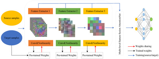
Figure 4.
Transfer learning framework.
Specifically, in this paper, the procedure of transfer learning could be described as follows. Firstly, we used the source dataset to start our training and obtained a pre-trained model Mpre, which contains the weight values and other feature information learned from the source data. Notice that all the learned weights are regarded as the initial settings of the network. Then, we input the limited target samples for training by setting the learned parameters in each feature extractor. For example, when transferring the parameters learned from Feature Extractor 2, we configure the learning rate in Extractor 1 and 2 (before Extractor 3) to zero or smaller values, the parameters in Extractor 3 keep the same initialization to yield the model Mtest. Finally, the model is used for the SAR ATR tasks. In our work, we explored the performance by transferring different feature extractors and the results of the experiment are shown.
4. Experimental Results and Analysis
All the experiments here were conducted with Intel Core i7-9700K CPU in a Windows 10 operation system. The computer was configurated with NVIDIA GTX 2070 and 16G RAM. The experiments were implemented with the public TensorFlow framework.
4.1. MSTAR Dataset
MSTAR is a quintessential and widely researched dataset which majors in recognizing the SAR targets. In this paper, it was adopted for experimental evaluation. The dataset contained ten classes of targets listed in Table 2, each class of which were sampled from a 15°/17° depression angle, respectively. The SAR images from this dataset are displayed in Figure 5. For the convenience of recording, all the experiments are conducted for classification based on the dataset above.
Table 2.
The training and test datasets.
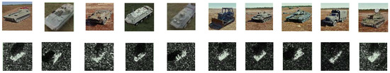
Figure 5.
SAR Images Instance in MSTAR Dataset.
4.2. Performance Evaluation
In this section, experiments were carried out to validate the model performance from various aspects. Figure 6 displays the visualization of features extracted from each layer, from which we observed that the network is capable of extracting robust and discriminative features. As a basic component of the network, an insight into the network will be rendered to explore the characteristics by analyzing various settings in this section.
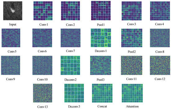
Figure 6.
Visualization of MFFA-SARNET layers.
4.2.1. Evaluation on Attention Module
For CNN, which inputs 2D images, one dimension is the image’s scale space, referring to the length and width, and the other dimension is the common mechanism with channel-based Attention. The essence of channel attention mechanism is that it models the importance of each feature, and assigns the feature to different tasks according to the input with ease and effectiveness. In spatial attention, though not all regions in the image are equally important to the task, the regions related to the task, such as the subject of the classification task, deserve core attention paid to them in order to find the most important part of the network for processing.
Reading from Experiments 1 to 4 in Table 3, the best performance belongs to the network with channel–spatial attention module at 98.5%, slightly increasing by 0.9% and 0.7%, respectively, compared to the network with channel attention and spatial attention separately. Data prove that the present results positively correlate with the existence of the weighting mechanism in all dimensions in Experiment 4. In contrast, due to the absence of a weighting mechanism both in the first two dimensions in Experiment 2 and the third dimension in Experiment 3, inferior accuracy occurs. The attention maps of some instances are presented in Figure 7. Furthermore, to acquire in-depth knowledge of the attention module, comparisons of several attention modules have been implemented in the network. Judging from the outcomes of the comparisons, the number of attention modules shares a negative correlation with the corresponding performance, which can be mainly attributed to the distracting influence that attention modules impose on the weighted effect.
Table 3.
Performance of attention module (ELU).
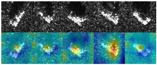
Figure 7.
The attention maps of some instances.
4.2.2. Activation Ablation Study
The activation function is mostly employed to fit different functions according to different classification tasks, especially nonlinear functions. The sigmoid function, also known as the S function, used to map variables between 0 and 1, gives a positive probability of interpreting the results of the algorithm. Unfortunately, it possesses a disadvantage—when inputting a large positive or negative number, the derivative will become zero and the gradient descent method will decline slowly, causing dysfunction in the neural network’s normal update. Even though the Tanh function can limit values, the slop approximates to zero when the z value is large or small, which overwhelmingly delays the optimization. The ReLU function, also called the linear rectification function, not only solves the problem of an abnormal parameter update when the gradient is zero under large value conditions, but also owns no complex exponential calculation. The softmax function shares a similarity with sigmoid function in that it can transform values to zero or one, but the softmax function is usually adopted in classifiers because the normalized probability of each category can be predicted for multiple categories. Moreover, ELU and CReLU are the variances of ReLU.
In Figure 8, we notice that cReLU, ELU, and ReLU6 achieved comparatively satisfying performances among eight subjects, among which the accuracy of the Tanh function at 96.8% surpasses those of both sigmoid and Softplus activation functions. A similar result is also obtained by the function Softsign at 96%. Compared with the performance of sigmoid, those of ELU, cReLU, and ReLU6 realize a growth of 8.8%, 8.5% and 8.5%, respectively. In the next section, the evaluation of loss functions is conducted on the network implemented with ELU/cReLU/ReLU6 on the basis of unfavorable performance in the proposed network.
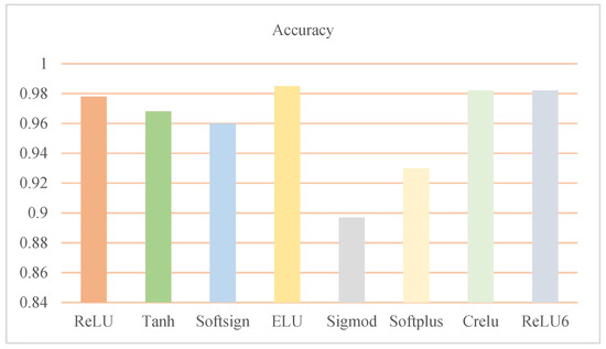
Figure 8.
Performance of various activation functions.
4.2.3. Evaluation of Loss Function
Loss function, as an objective function of optimization, is applied to evaluate the degree of inconsistency between the predicted value and the ground truth under most of the situations. The process of training or optimizing in the network refers to the operation of minimizing the loss function. The losses shown in Table 4 reflect the superiority of the method mentioned in this paper. In quadratic loss function, as its name suggests, the square loss function, often used in linear regression tasks, is the square of the difference between the predicted value and the ground truth. This means that the greater the loss, the greater the difference between the predicted value and the ground truth. To better ensure the evaluation’s accuracy, several self-defined combined loss functions described in Table 4 are adopted in this paper.
Table 4.
Loss function comparison.
Clearly, from Table 5, comparing the data of basis separate loss with those of the proposed method, we can conclude that adding SSIM can effectively contribute growth to the performance, with the highest accuracy at 98.5%. To further explore the proposed loss function as a whole, we also review the performance of various loss functions based on several activation functions. In Table 6, the results state that our proposed method outperforms other loss functions when using the cReLU, ELU and ReLU6 activation functions, with an accuracy of up to 98.5%. In each row, all performances listed are comparatively satisfied except for MSE, AVE and the designed Loss Function 1, which stand at unfavorable recognition rates under 80%. Though the other methods reach a comparatively gratifying accuracy, they still seem to be slightly inferior to that of the proposed method. All the results have testified that our proposed network with the presented loss defeats other methods.
Table 5.
Performance of loss function based on the proposed loss function.
Table 6.
Performance on various loss functions based on cReLU/ELU/ReLU6.
4.2.4. Evaluation of Multi-Level Feature Fusion
In order to certify the effectiveness of our feature fusion method implemented in the network for improving the classification performance, we conducted the experiments with the designed network shown in Figure 9 and renamed different networks in the experiment Net1 (our proposed network), Net2 and Net3, with the latter two networks being modified according to Net1, with their performances illustrated in Table 7.
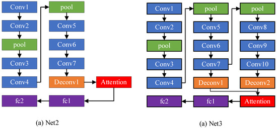
Figure 9.
The structure of Net2 and Net3.
Table 7.
Performance of feature fusion.
Table 7 appears to show that the single feature branch from Net2 reaches an accuracy of 96.3%, smaller than the other two feature branches. The results have demonstrated that our feature fusion method, with a recognition rate of about 98.5%, triumphs over the other feature fusion methods like Net2 and Net3. In an array of works, the fusion of features of different scales acts as a crucial means to improve segmentation performance. As learned from the above experiment, we observed that the low-level feature contains more detailed information of SAR images, while suffering from a large amount of noise, which degrades the performance of recognition. Our proposed feature fusion method contributes to boosting the performance of the SAR classification task.
4.3. Experiments under SOC
In this work, experiments under standard operating conditions (SOC) were conducted based on the MSTAR dataset displayed in Table 2. In the experiments’ configuration, variations BMP2_9563 and T72_132 are considered to be the corresponding classes. For instance, series 9563 and 132 are included in the class for training. The confusion matrix under SOC is shown in Table 8.
Table 8.
Confusion matrix of the proposed method under the ten targets based on standard operating conditions (SOC).
Information from Table 8 tells us that the percentage of correction classification for six targets was 100%, the Percentage of Correction Classification (PCC) of the rest of the targets was over 90%, and the average accuracy was up to 98.5%. Tan [40] presented a method to match the attribute scattering center with the binary target region, the performance of which was about 98.3%, less than that of our proposed method by 0.3%. For the Support Vector Machines (SVM) [41], the feature vectors are extracted by PCA with performance of SAR ATR at about 95.6%. Sparse Representation-based Classifier (SRC) [42] is a method using the Orthogonal Matching Pursuit (OMP) algorithm to solve the SAR ATR task with an accuracy of about 94.6%, while A-ConvNet [43] using the CNN model is engaged with a better performance at about 97.5%. Methods such as Attributed Scattering Centers (ASC) Matching [44], Region Matching [45], and other state-of-the-art methods obtain comparatively satisfactory results, as illustrated in Table 9. From all of these results, it is clear that even CNN is effective enough to solve the classification task, even though its performance also suffers from insufficient samples, which leads to insufficient feature extraction and inferior classification performance. The proposed method combines shallow, middle and high semantic features to accomplish the SAR ATR task and perform the best when comparisons are made with other methods under SOC.
Table 9.
Performance of all the methods under SOC.
4.4. Experiment under EOC-Large Depression Angle Variation
To deepen our understanding of the proposed network, experiments on Extended Operating Conditions (EOC) large depression angle variation were also implemented in Table 10. We collected the three classes, 2S1, BDRM2 and ZSU23/4 under 17° depression as the training dataset, and those under 30°/45° as the testing dataset to validate our proposed method. Obviously, Table 11 shows that the performance of a larger depression angle 45°, at about 90.1%, is inferior to that of the 30° angle. It is clear that the larger the depression angle variations are, the bigger the change in the appearance of the imaging object, thus resulting in an inferior performance in the SAR ATR task. We also made quite a few comparisons with other previous studies, displayed in Table 12, with the conclusion that our proposed method outperforms other methods under both configurations of 30°and 45°. Observations from Table 11 and Table 12 demonstrate that our proposed network possesses a better ability to make classifications under various depression angles.
Table 10.
The dataset with large depression angle variations.
Table 11.
Classification results of proposed method at 30° and 45° depression angles.
Table 12.
Comparisons with other methods to the EOC.
4.5. Experiments under Transfer Learning
Extensive experiments were conducted in this section via introducing the transfer learning method. To begin with, we pre-trained and optimized the eight classes in the MSTAR dataset without the classes BMP2 and T72 with the accuracy reaching 98.5%. In the interest of validating the superiority of our proposed method, we also employed the proposed network to test the variances in the classes BMP2 and T72, whose performances of classification stand at 79.8% and 92.6%, respectively, as presented in Table 13. Then, we divided the network into three branches, Net1, Net2, and Net3, which were used to transfer the weights learned from the SAR8. At length, we fine-tuned the parameters based on the target dataset. Table 14 shows the best performance in two classes when transferring the weights of Net1, rising by about 12.6% and 2.4%, respectively, compared to the situation where the transfer learning method was not used. This proves that the transfer learning method is able to support the network to learn more robust features from SAR images.
Table 13.
Performance of SAR8/BMP2/T72.
Table 14.
Transferring performance of SAR8/BMP2/T7.
4.6. Experiments under Small Established Dataset on SOC and EOC
For the purpose of validating the robustness of our proposed method, we also set a new configuration to explore the performance of the SAR ATR task. We selected 1/32, 1/16, 1/8, 1/4, 1/3 and 1/2 images from the corresponding classes randomly and tested the classification performance on the established dataset. As is shown in Table 15 and Table 16, compared with those state-of-the-art methods, the performance of our proposed method surpasses other ones in the SAR ATR task, and the network can make full use of the learned fused robust features to deal with the classification task. Experimental results certify that our proposed network can mitigate the limitation of insufficient training samples in classification by using the deep learning method, engendering a satisfying classification performance.
Table 15.
Experiments under small established datasets on SOC.
Table 16.
Experiments under small established dataset on EOC.
5. Conclusions
In this paper, a deep transferred multi-level feature fusion attention network with dual optimized loss for small-sample SAR ATR tasks is proposed, which can efficiently enhance the discriminative power of feature representation learned from the proposed network. The multi-level feature fusion attention network serves as the basis for viewing the learned features of targets as fused features. The dual optimized loss is employed to refine the intra-class compactness and inter-class separation and strengthen the similarity of each class, indicating that the loss is capable of improving the discriminative power of features. All the comprehensive experiments have demonstrated that the proposed scheme consistently outperformed the state-of-the-art ones and received a gratifying performance on the small-sample database, justifying the effectiveness and robustness of our proposed network significantly. In the near future, meta learning will be further investigated regarding the problems of limited training samples and highly expensive labeling costs for large scale SAR ATR.
Author Contributions
Y.Z. and W.D. wrote the paper. Y.Z. and J.L. conceived of and designed the experiments. W.D. and T.L. performed the experiments, J.G. and Z.Y. collected the data. B.S. and C.M. analyzed the experimental results. R.D.L., V.P., and F.S. revised the paper. All authors have read and agreed to the published version of the manuscript.
Funding
This research was funded by the National Natural Science Foundation of China under Grant 61771347, in part by the Guangdong Basic and Applied Basic Research Foundation under Grant 2019A1515010716, in part by the Characteristic Innovation Project of Guangdong Province under Grant 2017KTSCX181, in part by the Open Project of Guangdong Key Laboratory of Digital Signal Processing Technology (No. 2018GDDSIPL-02), and in part by the Basic Research and Applied Basic Research Key Project in General Colleges and Universities of Guangdong Province under Grant 2018KZDXM073, Special Project in key Areas of Artificial Intelligence in Guangdong Universities (No.2019KZDZX1017), Open fund of Guangdong Key Laboratory of digital signal and image processing technology (2019GDDSIPL-03).
Acknowledgments
In this section you can acknowledge any support given which is not covered by the author contribution or funding sections. This may include administrative and technical support, or donations in kind (e.g., materials used for experiments).
Conflicts of Interest
The authors declare no conflict of interest.
References
- Ahishali, M.; Kiranyaz, S.; Ince, T.; Moncef, G. Dual and Single Polarized SAR Image Classification Using Compact Convolutional Neural Networks. Remote Sens. 2019, 11, 1340. [Google Scholar] [CrossRef]
- Ding, J.; Chen, B.; Liu, H.; Huang, M. Convolutional neural network with data augmentation for SAR target recognition. IEEE Geosci. Remote Sens. Lett. 2016, 13, 364–368. [Google Scholar] [CrossRef]
- Matteoli, S.; Diani, M.; Corsini, G. Automatic Target Recognition Within Anomalous Regions of Interest in Hyperspectral Images. IEEE J. Sel. Top. Appl. Earth Obs. Remote Sens. 2018, 11, 1056–1069. [Google Scholar] [CrossRef]
- Wang, H.; Li, S.; Zhou, Y.; Chen, S. SAR Automatic Target Recognition Using a Roto-Translational Invariant Wavelet-Scattering Convolution Network. Remote Sens. 2018, 10, 501. [Google Scholar] [CrossRef]
- Chi, J.; Yu, X.; Zhang, Y.; Huan, W. A Novel Local Human Visual Perceptual Texture Description with Key Feature Selection for Texture Classification. Math. Probl. Eng. 2019, 2019, 1–20. [Google Scholar] [CrossRef]
- Cheng, G.; Han, J.; Lu, X. Remote sensing image scene classification: Benchmark and state of the art. Proc. IEEE 2017, 105, 1865–1883. [Google Scholar] [CrossRef]
- Yu, Q.; Zhou, S.; Jiang, Y.; Peng, W.; Yong, X. High-Performance SAR Image Matching Using Improved SIFT Framework Based on Rolling Guidance Filter and ROEWA-Powered Feature. IEEE J. Sel. Top. Appl. Earth Obs. Remote Sens. 2019, 12, 920–933. [Google Scholar] [CrossRef]
- Liu, H.; Wang, F.; Yang, S.; Hou, B.; Jiao, L.; Yang, R. Fast Semi-supervised Classification Using Histogram-Based Density Estimation for Large-Scale Polarimetric SAR Data. IEEE Geosci. Remote Sens. Lett. 2019, 16, 1844–1848. [Google Scholar] [CrossRef]
- Ghannadi, M.A.; Saadaseresht, M. A Modified Local Binary Pattern Descriptor for SAR Image Matching. IEEE Geosci. Remote Sens. Lett. 2018, 16, 568–572. [Google Scholar] [CrossRef]
- Pei, J.; Huang, Y.; Huo, W.; Zhang, Y.; Yang, J.; Yeo, T.S. SAR automatic target recognition based on multiview deep learning framework. IEEE Trans. Geosci. Remote Sens. 2017, 56, 2196–2210. [Google Scholar] [CrossRef]
- Eryildirim, A.; Cetin, A.E. Man-made object classification in SAR images using 2-D cepstrum. In Proceedings of the IEEE Radar Conference, Pasadena, CA, USA, 4–8 May 2009. [Google Scholar] [CrossRef]
- Clemente, C.; Pallotta, L.; Gaglione, D.; De Maio, A.; Soraghan, J.J. Automatic Target Recognition of Military Vehicles with Krawtchouk Moments. IEEE Trans. Aerosp. Electron. Syst. 2017, 53, 493–500. [Google Scholar] [CrossRef]
- Sun, Y.; Du, L.; Wang, Y.; Wang, Y.; Hu, J. SAR Automatic Target Recognition Based on Dictionary Learning and Joint Dynamic Sparse Representation. IEEE Geosci. Remote Sens. Lett. 2016, 13, 1777–1781. [Google Scholar] [CrossRef]
- Kim, S.; Song, W.J.; Kim, S.H. Robust Ground Target Detection by SAR and IR Sensor Fusion Using Adaboost-Based Feature Selection. Sensors 2016, 16, 1117. [Google Scholar] [CrossRef] [PubMed]
- Lin, Z.; Ji, K.; Kang, M.; Leng, X.; Zou, H. Deep convolutional highway unit network for SAR target classification with limited labeled training data. IEEE Geosci. Remote Sens. Lett. 2017, 14, 1091–1095. [Google Scholar] [CrossRef]
- Sharifzadeh, F.; Akbarizadeh, G.; Kavian, Y.S. Ship classification in SAR images using a new hybrid CNN–MLP classifier. J. Indian Soc. Remote Sens. 2019, 47, 551–562. [Google Scholar] [CrossRef]
- Tian, Z.; Wang, L.; Zhan, R.; Hu, J.; Zhang, J. Classification via weighted kernel CNN: Application to SAR target recognition. Int. J. Remote Sens. 2018, 39, 9249–9268. [Google Scholar] [CrossRef]
- Ma, M.; Chen, J.; Liu, W.; Wei, Y. Ship Classification and Detection Based on CNN Using GF-3 SAR Images. Remote Sens. 2018, 10, 2043. [Google Scholar] [CrossRef]
- Espinal, F.; Huntsberger, T.; Jawerth, B.D.; Kubota, T. Wavelet-based fractal signature analysis for automatic target recognition. Opt. Eng. 1998, 37, 166–174. [Google Scholar] [CrossRef]
- Huan, R.H.; Pan, Y.; Mao, K.J. SAR image target recognition based on NMF feature extraction and Bayesian decision fusion. In Proceedings of the 2010 Second IITA International Conference on Geoscience and Remote Sensing, Qingdao, China, 28–31 August 2010; pp. 496–499. [Google Scholar] [CrossRef]
- Chamundeeswari, V.V.; Singh, D.; Singh, K. An analysis of texture measures in PCA-based unsupervised classification of SAR images. IEEE Geosci. Remote Sens. Lett. 2009, 6, 214–218. [Google Scholar] [CrossRef]
- Sakarya, U.; Demirpolat, C. SAR image time-series analysis framework using morphological operators and global and local information-based linear discriminant analysis. Turk. J. Electr. Eng. Comput. Sci. 2018, 26, 2958–2966. [Google Scholar] [CrossRef]
- Zhou, Y.; Chen, Y.; Gao, R.; Feng, J.; Zhao, P.; Wang, L. SAR Target Recognition via Joint Sparse Representation of Monogenic Components With 2D Canonical Correlation Analysis. IEEE Access 2019, 7, 25815–25826. [Google Scholar] [CrossRef]
- Yu, M.; Quan, S.; Kuang, G.; Ni, S. SAR Target Recognition via Joint Sparse and Dense Representation of Monogenic Signal. Remote Sens. 2019, 11, 2676. [Google Scholar] [CrossRef]
- Yann, L.; Yoshus, B.; Geoffrey, H. Deep Learning. Nature 2015, 521, 436–444. [Google Scholar] [CrossRef]
- Yoshua, B. Learning Deep Architectures for AI. Found. Trends Mach. Learn. 2009, 2, 35–37. [Google Scholar] [CrossRef]
- Lecun, Y.; Bottou, L.; Begio, Y. Gradient based learning applied to document recognition. Proc. IEEE 1998, 86, 2278–2324. [Google Scholar] [CrossRef]
- Krizhevsky, A.; Sutskever, I.; Hinton, G.E. ImageNet classification with deep convolutional neural networks. NIPS 2012, 1106–1114. [Google Scholar] [CrossRef]
- Zhang, F.; Wang, Y.; Ni, J.; Zhou, Y.; Hu, W. SAR Target Small Sample Recognition Based on CNN Cascaded Features and AdaBoost Rotation Forest. IEEE Geosci. Remote Sens. Lett. 2019. [Google Scholar] [CrossRef]
- Liu, H.; Shang, F.; Yang, S.; Gong, M.; Zhu, T.; Jiao, L. Sparse Manifold-Regularized Neural Networks for Polarimetric SAR Terrain Classification. IEEE Trans. Neural Netw. Learn. Syst. 2019, 1–10. [Google Scholar] [CrossRef]
- Amrani, M.; Jiang, F. Deep feature extraction and combination for synthetic aperture radar target classification. J. Appl. Remote Sens. 2017, 11, 042616–042634. [Google Scholar] [CrossRef]
- Wang, N.; Wang, Y.; Liu, H.; Zuo, Q.; He, J. Feature-fused SAR target discrimination using multiple convolutional neural networks. IEEE Geosci. Remote Sens. Lett. 2017, 14, 1695–1699. [Google Scholar] [CrossRef]
- Zheng, C.; Jiang, X.; Liu, X.Z. Generalized synthetic aperture radar automatic target recognition by convolutional neural network with joint use of two-dimensional principal component analysis and support vector machine. J. Appl. Remote Sens. 2017, 11, 046007–046020. [Google Scholar] [CrossRef]
- Yu, Q.; Hu, H.; Geng, X.; Jiang, Y.; An, J. High-Performance SAR Automatic Target Recognition Under Limited Data Condition Based on a Deep Feature Fusion Network. IEEE Access 2019, 7, 165646–165658. [Google Scholar] [CrossRef]
- Huang, Z.; Pan, Z.; Lei, B. Transfer learning with deep convolutional neural network for SAR target classification with limited labeled data. Remote Sens. 2017, 9, 907. [Google Scholar] [CrossRef]
- Rostami, M.; Kolouri, S.; Eaton, E.; Kyungnam, K. Deep Transfer Learning for Few-Shot SAR Image Classification. Remote Sens. 2019, 11, 1374. [Google Scholar] [CrossRef]
- Xu, Y.; Lang, H.; Niu, L.; Ge, C. Discriminative Adaptation Regularization Framework-Based Transfer Learning for Ship Classification in SAR Images. IEEE Geosci. Remote Sens. Lett. 2019, 16, 1786–1790. [Google Scholar] [CrossRef]
- Chen, S.; Wang, H.; Xu, F.; Jin, Y.Q. Target classification using the deep convolutional networks for SAR images. IEEE Trans. Geosci. Remote Sens. 2016, 54, 4806–4817. [Google Scholar] [CrossRef]
- Tan, J.; Fan, X.; Wang, S.; Ren, Y. Target Recognition of SAR Images via Matching Attributed Scattering Centers with Binary Target Region. Sensors 2018, 18, 3019. [Google Scholar] [CrossRef]
- Wilmanski, M.; Kreucher, C.; Lauer, J. Modern approaches in deep learning for SAR ATR. In Proceedings of the SPIE 9843 Algorithms for Synthetic Aperture Radar Imagery XXIII, Baltimore, MD, USA, 17–21 April 2016; p. 98430N. [Google Scholar] [CrossRef]
- Zhao, Q.; Principe, J.C. Support vector machines for SAR automatic target recognition. IEEE Trans. Aerosp. Electron. Syst. 2001, 37, 643–654. [Google Scholar] [CrossRef]
- Song, H.; Ji, K.; Zhang, Y.; Xing, X.; Zou, H. Sparse representation-based SAR image target classification on the 10-class MSTAR data set. Appl. Sci. 2016, 6, 26. [Google Scholar] [CrossRef]
- Du, K.; Deng, Y.; Wang, R.; Tuan, Z.; Ning, L. SAR ATR based on displacement-and rotation-insensitive CNN. Remote Sens. Lett. 2016, 7, 895–904. [Google Scholar] [CrossRef]
- Ding, B.; Wen, G.; Huang, X.; Ma, C.; Yang, X. Target recognition in synthetic aperture radar images via matching of attributed scattering centers. IEEE J. Sel. Top. Appl. Earth Obs. Remote Sens. 2017, 10, 3334–3347. [Google Scholar] [CrossRef]
- Ding, B.; Wen, G.; Ma, C.; Yang, X. Target recognition in synthetic aperture radar images using binary morphological operations. J. Appl. Remote Sens. 2016, 10, 046006–046020. [Google Scholar] [CrossRef]


© 2020 by the authors. Licensee MDPI, Basel, Switzerland. This article is an open access article distributed under the terms and conditions of the Creative Commons Attribution (CC BY) license (http://creativecommons.org/licenses/by/4.0/).