City-Scale Distance Sensing via Bispectral Light Extinction in Bad Weather

Abstract

In this paper, we propose a novel city-scale distance sensing algorithm based on atmosphere optics. The suspended particles, especially in bad weather, would attenuate the light at almost all wavelengths. Observing this fact and starting from the light scattering mechanism, we derive a bispectral distance sensing algorithm by leveraging the difference of extinction coefficient between two specifically selected near infrared wavelengths. The extinction coefficient of the atmosphere is related to both wavelength and meteorological conditions, also known as visibility, such as the fog and haze day. To account for different bad weather conditions, we explicitly introduce visibility into our algorithm by incorporating it into the calculation of extinction coefficient, making our algorithm simple yet effective. To capture the data, we build a bispectral imaging system that is able to take a pair of images with a monochrome camera and two narrow band-pass filters. We also present a wavelength selection strategy that allows us to accurately sense distance regardless of material reflectance and texture. Specifically, this strategy determines two distinct near infrared wavelengths by maximising the extinction coefficient difference while minimizing the influence of building’s reflectance variance. The experiments empirically validate our model and its practical performance on the distance sensing for the city-scale buildings.

1. Introduction

When light travels from its source (e.g., the surface of a building) to the destination (e.g., a camera), its interaction with the atmosphere would inevitably alter its characteristics like intensity and colour, or more precisely, the spectral energy distribution. This phenomena, severe especially in bad weather, would violate the basic assumption of standard vision that air is transparent. Generally regarded as the hindrance, the computational photography community has made much effort in removing rain and fog [1,2,3,4,5,6]. Just like every cloud has a silver lining, some seminar progress [1,7] instead analysed the visual effects of bad weather to encode the scene structure, such as depth. One of the most seminal attempts was made by Srinivasa et al. [7]. Assuming the scenario in the dense fog, Srinivasa et al. [7] proposed to recover the depth structure from the airlight in a single image. However, this method only works on the heavy fog and close distance. Srinivasa et al. [7] also tried to estimate the depth by comparing the extinction of two different weather condition (e.g., a clear day and a bad weather) images from exactly the same viewpoint. Taking two images at two different weather conditions requires some effort owing to the fact that the weather may be unchanged for some time (e.g., several hours). The requirement of image pair significantly restricts its actual application.

In this paper, we propose a novel city-scale distance sensing algorithm from a snapshot under bad weather. To this end, we build a bispectral imaging system utilizing a simple monochrome camera equipped with two narrow band-pass filters (Model: 905 nm and 980 nm CWL, 50 mm Dia., Hard Coated OD 4 10 nm Bandpass Filter). This prototype almost allows us to simultaneously capture a pair of monochromatic images at two specific near infrared wavelengths.

With the captured bispectral image pair and extinction coefficients, our relative distance sense algorithm, shown in Figure 1, is able to sense the city-scale distance by exploring the light propagation and meteorological condition. When light travels through the atmosphere, it is usually attenuated due to its interactions with the suspended particles [7,8,9] at certain wavelengths. With the Beer-Lambert law, attenuation at a certain wavelength is proportioned to both the length of the light propagation path and the extinction coefficient of the atmosphere [9,10]. The extinction coefficient is varied in different weather conditions and wavelengths. By introducing the visibility, publicly available in routine meteorological reports, we are able to explicitly calculate the extinction coefficient according to the weather condition and wavelength, which allows us to directly sense the distance from a surface point in a building to the camera through the degree of light attenuation and weather condition.

Our distance sensing method is based on a pair of images captured at two different wavelengths and two extinction coefficients. Inspired by previous task-specific spectral wavelength selection research [11], we select two distinct wavelengths that maximise the light attenuation difference while minimizing the influence of reflectance in the city-scale buildings. Specifically, we empirically demonstrate that the reflectance curve of common materials in urban buildings appeared to be flat under near infrared wavelengths (e.g., 900 ~1000nm). The evidence could also be supported in [11]. Meanwhile, around these wavelengths, the near infrared light is still sufficient for our analysis and computation even though it is being attenuated.

With two extinction coefficients calculated from the visibility and two wavelengths, we could finally estimate the distance. As illustrated in Figure 1, in the proposed bispectral distance sensing algorithm, the input data includes a pair of images and visibility in bad weather. The image pair is captured at 905 and 980 nm, respectively. The output result is the estimated relative distance. To make the computation tractable, the visibility is obtained from a routine meteorological report. Moreover, the global atmosphere light intensity can be estimated utilising the input near infrared images. In addition, two extinction coefficients can be computed using two chosen wavelengths and visibility. Experimental results demonstrate the effectiveness of theory and the actual implementation of this novel algorithm.

Our main contributions of this paper are three-fold:

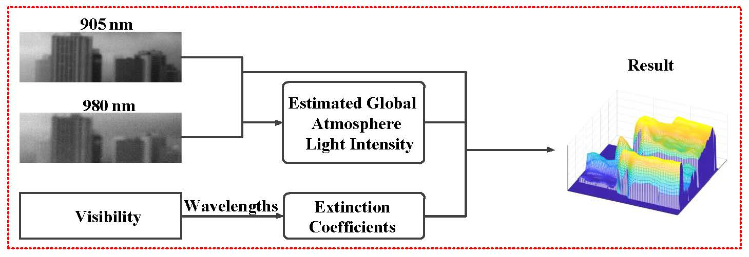
• We propose a novel framework to directly estimate the city-scale distance in bad weather by taking advantage of bispectral light extinction.
• We incorporate the visibility into our light attenuation model to account for the weather condition. By our knowledge, this is the first attempt to explicitly model the atmosphere interaction by visibility, an easily accessible meteorological data.
• We construct an actual bispectral imaging system and validate the superior performance of our method.

The remainder of this paper is organized as follows. In Section 2, we review the related works. Section 3 briefly describes the physical model based on the mechanisms of light scattering. In Section 4, we introduce details of the bispectral light extinction algorithm in the task of distance sensing. In Section 5, experiment results are presented to verify the practical performance of the proposed algorithm on near infrared images pairs. Finally, we draw the discussion and conclusions in Section 6 and Section 7, respectively.

2. Related Works

Distance sensing is an essential technique for computer vision [12], robotics [13,14], 3D reconstruction [15,16], and computer graphics [17], etc. One popular distance sensing algorithm is called time of flight [18], which measures the travel time of a light pulse to hit a surface and go back to the source. Time of flight can be directly used to encode the distance of the surface of an object from the source. However, accurate measurement of the time of flight requires special hardware. Given the images acquired by the cameras, methods such as binocular, multi-view stereo, and structure from motion [19,20] exploit the fundamental geometric relationship to estimate the distance. These methods rely on finding and matching the unique texture characteristic on the surface of the object, making them vulnerable to the noises. Shape-from-shading [21] and photometric stereo [22] infer the distance by modelling the changing of surface brightness. However, their performances are limited to the object with texture and complex reflectance.

Srinivasa et al., in their seminar works [7,9,10], proposed to estimate the depth cue from chromatic decomposition model on attenuation. The proposed method requires two RGB images under different weather conditions (e.g., a thinner and a denser fog), which have different attenuation coefficients from the same viewpoint. However, it is time-consuming to capture these two images in a short period of time taking into account that weather condition varies slowly. By assuming the airlight dominates the scattering effect, such as in heavy fog, [7,10] could also work on a single image. However, this estimation would deteriorate and even fail under clearer weather conditions. Furthermore, its assumption that each wavelength shares the same extinction coefficient is far from realistic. For example, the sky looks blue due to the wavelength-dependent scattering, Rayleigh scattering [23]. After [7], some progress has been made on depth sensing from a single image. For instance, Tan [24] has found that images without haze always have higher contrast. He maximizes the local contrast of the processed image to estimate depth. He et al. [1] also modelled the visual effect of haze to remove it from a single image using a dark channel prior, which is a kind of statistics of the haze-free outdoor images, and obtained a depth map. The method from [1] can work well based on a key observation—most local patches in haze-free outdoor images contain some pixels which have very low intensities in at least one colour channel. Although the above methods achieve progress on depth sensing based on some priors, they usually ignore the actual meteorological parameters.

The depth sensing also can be formulated as a supervised regression problem given a large training dataset. These methods attempt to directly predict the distance of each pixel in the image using a trained offline model [12,25,26,27,28,29]. For example, Saxena et al. [25] introduced a model based on the patch dubbed as Make3D to estimated the 3D location and orientation of local planes. The predictions of plane parameters are obtained by utilizing the linear model trained offline before MRF post-processes. Liu et al. [27] learned the depth sensing with a convolutional neural network. Karsch et al. [17] proposed to produce more consistent image level predictions by copying the whole depth image from the training set. Ladicky et al. [28] attempted to incorporate a semantic into the model to ameliorate the sensed depth of each pixel. Although enjoying quiet success, these supervised methods are limited by the requirement of a large training dataset. Therefore, Flynn et al. [30] proposed an unsupervised depth estimation method. They introduced a new image synthesis network called Deep-Stereo, which can generate new views by selecting pixels from several nearby posed images. However, all of these methods only work on a clear day.

Recently, Asano et al. [11] utilized the bispectral light absorption for depth sensing under water. Specifically, they measured the absorption coefficient of water in a laboratory environment. Inspired by this work, we propose a novel city-scale distance sensing algorithm using a bispectral distance sensing imaging system similar to [11]. Here, we study the physical model of the atmosphere’s interaction with light due to the suspended particles. Instead of the laboratory measurement, we infer the atmosphere condition through visibility, a parameter publicly available in a daily weather report. By our knowledge, this is the first research that models bad weather using visibility.

3. Mechanisms of Light Scattering

It is well known that light scattering will occur in bad weather because of the light’s interactions with the suspended particles in the atmosphere [7,8,9]. Our proposed distance sensing method is based on the mechanisms of light scattering. In this section, we will introduce the atmosphere scattering model that comprises of two fundamental and essential scattering phenomena: attenuation and airlight. We derive this atmosphere scattering model from [7,8,9,10,31].

Attenuation Phenomenon When travelling through the medium such as air or water, light would be attenuated. Under foggy weather conditions, the medium is mainly water droplets. According to the Beer–Lambert law, the decay of light power will comply with the exponential decay law. The observed attenuated light power intensity $E(\lambda ,d)$ can be calculated as follows:

$$E(\lambda ,d)=J\left(\lambda \right)e^{-{\beta }_e\left(\lambda \right)d},$$

(1)

where $\lambda$ is the wavelength of light, and d is the relative distance between building and camera. $J\left(\lambda \right)$ represents the object radiance intensity that equals the product of reflectance spectra of material and the airlight spectra. ${\beta }_e\left(\lambda \right)$ means the extinction coefficient that we aim to infer from the wavelength and visibility.

Airlight Phenomenon The airlight comes from the scattered environmental illumination (e.g., sunlight) by the particles in the atmosphere. This phenomenon contributes to the blue or foggy sky. The airlight will increase the power radiation intensity received by the camera. The increased light power intensity $L(\lambda ,d)$ can be computed as follows:

$$L(\lambda ,d)=A\left(\lambda \right)(1-e^{-{\beta }_e\left(\lambda \right)d}),$$

(2)

where $A\left(\lambda \right)$ is the global atmosphere light intensity. It equals the airlight radiation intensity at the horizon that can be observed.

According to two important scattering phenomena above, the final light power intensity $I(\lambda ,d)$ received by camera can be expressed as:

$$I(\lambda ,d)=E(\lambda ,d)+L(\lambda ,d).$$

(3)

Substituting Equations (1) and (2) into Equation (3) and computing $J\left(\lambda \right)$ as $s\left(\lambda \right)$ multiplies $A\left(\lambda \right)$, we can obtain:

$$I(\lambda ,d)=s\left(\lambda \right)A\left(\lambda \right)e^{-{\beta }_e\left(\lambda \right)d}+A\left(\lambda \right)(1-e^{-{\beta }_e\left(\lambda \right)d}),$$

(4)

where $s\left(\lambda \right)$ is reflectance spectra of material. We can estimate $A\left(\lambda \right)$ utilizing the intensity of the sky without occlusion objects.

Solving d via Equation (4) is an under-constrained problem and requires specific values of $s\left(\lambda \right)$ and ${\beta }_e\left(\lambda \right)$. In the next chapter we will discuss how to obtain the two parameters above.

4. A Bispectral Light Extinction Algorithm for Distance Sensing

We aim at sensing the relative distance of city-scale buildings with respect to the camera in bad weather. Unlike the proposed methods in [7], we propose to capture two images under the same weather conditions at two selected near infrared wavelengths. By equipping two filters, two images could be obtained in less than 1 min, then we can estimate the relative distance quickly. Based on the model we described in Section 3, a bispectral light extinction distance sensing algorithm is proposed in this section.

4.1. Derivation of Distance Equation from Bispectral Light Imaging Theorem

Two images captured at two different wavelengths are utilized to estimate the relative distance. After selecting two different wavelengths, ${\lambda }_1$ and ${\lambda }_2$, for imaging and capturing a pair of images at the same viewpoint, we could obtain $I({\lambda }_1,d\left({\lambda }_1\right))$ and $I({\lambda }_2,d\left({\lambda }_2\right))$ by:

$$\begin{array}{c}\hfill I({\lambda }_1,d\left({\lambda }_1\right))=s\left({\lambda }_1\right)A\left({\lambda }_1\right)e^{-{\beta }_e\left({\lambda }_1\right)d\left({\lambda }_1\right)}+A\left({\lambda }_1\right)\left(1-e^{-{\beta }_e\left({\lambda }_1\right)d\left({\lambda }_1\right)}\right),\end{array}$$

(5)

$$\begin{array}{c}\hfill I({\lambda }_2,d\left({\lambda }_2\right))=s\left({\lambda }_2\right)A\left({\lambda }_2\right)e^{-{\beta }_e\left({\lambda }_2\right)d\left({\lambda }_2\right)}+A\left({\lambda }_2\right)\left(1-e^{-{\beta }_e\left({\lambda }_2\right)d\left({\lambda }_2\right)}\right).\end{array}$$

(6)

Equations (5) and (6) can be rewritten as follows:

$$\begin{array}{c}\hfill I({\lambda }_1,d\left({\lambda }_1\right))-A\left({\lambda }_1\right)=A\left({\lambda }_1\right)\left(s\left({\lambda }_1\right)-1\right)e^{-{\beta }_e\left({\lambda }_1\right)d\left({\lambda }_1\right)},\end{array}$$

(7)

$$\begin{array}{c}\hfill I({\lambda }_2,d\left({\lambda }_2\right))-A\left({\lambda }_2\right)=A\left({\lambda }_2\right)\left(s\left({\lambda }_2\right)-1\right)e^{-{\beta }_e\left({\lambda }_2\right)d\left({\lambda }_2\right)}.\end{array}$$

(8)

Two distances $d\left({\lambda }_1\right)$ and $d\left({\lambda }_2\right)$ at two different wavelengths can be calculated using Equations (7) and (8). The scene in front of the camera is identical for any pair of pixels in two different settings. Hence, we will have:

$$d=d\left({\lambda }_1\right)=d\left({\lambda }_2\right).$$

(9)

By dividing Equation (7) by Equation (8), the relative distance d can be expressed as:

$$d=\frac{ln\left(\frac{I\left({\lambda }_1,d\right)-A\left({\lambda }_1\right)}{I\left({\lambda }_2,d\right)-A\left({\lambda }_2\right)}\frac{A\left({\lambda }_2\right)}{A\left({\lambda }_1\right)}\frac{s\left({\lambda }_2\right)-1}{s\left({\lambda }_1\right)-1}\right)}{{\beta }_e\left({\lambda }_2\right)-{\beta }_e\left({\lambda }_1\right)}.$$

(10)

In Equation (10), $I\left({\lambda }_1,d\right),I\left({\lambda }_2,d\right),A\left({\lambda }_1\right)$, and $A\left({\lambda }_2\right)$ can be known from the image pair captured by the bispectral imaging system, and there are four unknown elements, which are $s\left({\lambda }_1\right),s\left({\lambda }_2\right),{\beta }_e\left({\lambda }_1\right)$, and ${\beta }_e\left({\lambda }_2\right)$. So at least four known relationships between four unknown elements need to be given if we want to calculate the relative distance. Here, if we can assume that $s\left({\lambda }_1\right)\approx s\left({\lambda }_2\right)$, then Equation (10) can be approximately expressed:

$$d\approx \frac{ln\left(\frac{I\left({\lambda }_1,d\right)-A\left({\lambda }_1\right)}{I\left({\lambda }_2,d\right)-A\left({\lambda }_2\right)}\frac{A\left({\lambda }_2\right)}{A\left({\lambda }_1\right)}\right)}{{\beta }_e\left({\lambda }_2\right)-{\beta }_e\left({\lambda }_1\right)}.$$

(11)

In Section 4.2, we will validate our assumption. In Section 4.3, we will introduce how to calculate ${\beta }_e\left({\lambda }_1\right)$ and ${\beta }_e\left({\lambda }_2\right)$.

4.2. Analysis of Spectral Reflectance of Material

To better solve the distance sensing problem on top of Equation (10), we form a simple yet effective assumption: $s\left({\lambda }_1\right)\approx s\left({\lambda }_2\right)$. Based on this assumption, we will demonstrate that only two extinction coefficients are required to compute the relative distance in this section. To validate this assumption, we investigate the reflectance spectra of both the standard colour checker board and common materials that appeared in the urban buildings, as shown in Figure 2. The standard colour checker board includes 24 different colour patches. The size of each colour patch is 3 × 3 cm, and the size of the other material patch is 12 × 12 cm.

Two spectrometers (Model:C10027-01, C10028-01), a standard white target for calibration, and an incandescent lamp (Model:PIS-UHX-AIR), which has sufficient near infrared irradiance, are used to measure the reflectance spectra of both the standard colour checker board and common materials in this section.

We used two spectrometers, which are spot sensors to measure the spectrum of a material as an average of an area of 1 cm square. The illumination spectrum was measured through the reflection on a Spectralon Diffuse Reflectance Standard by the same spectrometer. Then the reflectance spectrum of this material is obtained by dividing the spectrum of the material by the illumination spectrum.

The standard color checker board, which includes 24 different colours was chosen to examine its reflectance spectra, as shown in Figure 3a. We find that the reflectance spectra of standard colour checker board varies drastically when wavelengths are less than 900 nm. This implies different colours usually have a different reflectance spectrum in the wavelengths of visible range. From Figure 3a, we can also observe distinctly that the reflectance spectra of the standard colour checker board is almost flat when wavelengths are longer than 900 nm. In order to study the reflectance spectrum difference of different wavelengths, we calculate the spectrum difference using three reflectance spectrum pairs as follows:

$$\frac{s_{\lambda \in \left(920,950,980\right)}\left(\lambda \right)}{s\left(900\right)}-1.$$

(12)

where $s\left(900\right)$, $s\left(920\right)$, $s\left(950\right)$, and $s\left(980\right)$ represent the value of reflectance spectra at 900, 920, 950, 980, respectively.

As shown in Figure 3e, the average value of 24 patches’ spectrum difference in 920 nm with respect to 900 nm is $1.16\%$. It increases to $2.87\%$ in 950 nm with respect to 900 nm. The largest value is $4.63\%$ in 980 nm with respect to 900 nm. These spectrum differences can almost be neglected in the near infrared wavelength domain (e.g., 900 to 1000 nm), which supports the afore-mentioned claim for the standard colour checker board.

There are usually three classes of materials appearing on the city-scale buildings; stone, glass and metal. We collected 10 different stones, 20 different glasses, and 20 different metals to examine their reflectance spectra. The reflectance spectra of three classes materials mentioned above are drawn in Figure 3b–d. The reflectance spectrum difference is plotted in Figure 3f–h. The average spectrum difference of these three classes for the bispectral pair 980 and 900 nm is $3.11\%$, $11.13\%$, and $6.79\%$, respectively. For the bispectral pair 950 and 900 nm, the corresponding average spectrum difference reduces to $1.92\%$, $5.91\%$, and $4.41\%$. For the bispectral pair 920 and 900 nm, the corresponding average spectrum difference reduces to $1.12\%$, $1.85\%$, and $2.2\%$. Experiment statistics indicate that the reflectance spectra of three classes materials are very flat in the near infrared wavelengths and comply to our mild assumption $s\left({\lambda }_1\right)\approx s\left({\lambda }_2\right)$.

To analyze the error brought by this mild assumption, the relationship between the distance relative error $\Delta d$ and the reflectance spectrum relative error $\Delta s$ is analyzed here. $\Delta s$, defined as follows, is used to describe the difference between $s\left({\lambda }_1\right)$ and $s\left({\lambda }_2\right)$.

$$\Delta s=\frac{s\left({\lambda }_1\right)}{s\left({\lambda }_2\right)}-1.$$

(13)

Then $\Delta d$ can be calculated using Equations (10), (11), and (13) as follows:

$$\Delta d=\frac{ln\left(1+\frac{\Delta s}{1-\frac{1}{s_2}}\right)}{ln\left(1+\frac{\Delta s}{1-\frac{1}{s_2}}\right)-lnR},$$

(14)

where $R=\frac{I\left({\lambda }_1,d\right)-A\left({\lambda }_1\right)}{I\left({\lambda }_2,d\right)-A\left({\lambda }_2\right)}\frac{A\left({\lambda }_2\right)}{A\left({\lambda }_1\right)}$, can be seen as a constant.

Equation (14) demonstrates the relationship between $\Delta d$ and $\Delta s$. Variable-controlling approach is utilized in this section to study the relationship between $\Delta d$ and $\Delta s$. Only one of $s_2$ and R will be changed at a time. Figure 4a,c show the change of $\Delta d$ with $\Delta s$ when $s_2$/R is fixed at 0.2. Figure 4b,d are the first derivative (slope) of curves in Figure 4a,c. We find that, for most of curves, the absolute maximum of first derivative is no more than 0.4, indicating that $\Delta d$ is less sensitive to $\Delta s$ and our assumption in Section 4.2 is mild.

This gives us a criterion to choose the appropriate wavelengths to reduce unkowns. We should select the wavelengths of longer than 900 nm.

4.3. Calculation of Extinction Coefficient

To estimate d from Equation (11), we can compute ${\beta }_e\left({\lambda }_1\right)$ and ${\beta }_e\left({\lambda }_2\right)$ using the emprical extinction model derived in [32,33,34,35]. It is hard to calculate ${\beta }_e\left(\lambda \right)$ directly from the Mie scattering theory. This is because the actual size and number distribution of the particle is difficult to measure. The distribution usually varies in different climatic areas, environments, seasons, $etc.$ The empirical model related to the extinction coefficient is widely utilized in meteorology and it is attractive to calculate the extinction coefficient directly.

In [34,35], visibility is defined as the distance where the intensity of light reduces to $2\%$ of its initial value in 550 nm. The empirical model about the calculation of extinction coefficient can be formulated as follows [34,35]:

$${\beta }_e\left(\lambda \right)=\frac{3.91}{V}{\left(\frac{\lambda }{0.55}\right)}^{-q}\left({\mathrm{km}}^{-1}\right),$$

(15)

where V represents visibility and should be given in kilometers. V can be obtained in routine meteorological report. $\lambda$ should be given in micrometers, km means kilometer, and q is a parameter that is determined by V.

q in this empirical model can be estimated as follows:

$$q=\left\{\begin{array}{cc}0.585V^{\frac{1}{3}}& V<6\mathrm{km}\\ 1.3& 6\mathrm{km}\le V<50\mathrm{km}\\ 1.6& V\ge 50\mathrm{km}\end{array}\right..$$

(16)

The meteorological report department will announce visibility in different regions every day. However, in Japan, $5\%$ is usually used as the standard of visibility [36,37]. Thus, we could derive the formula again according to [34,35], and the number 3.91 in Equation (15) will become 2.9957. We could re-write Equation (15) as shown below:

$${\beta }_e\left(\lambda \right)=\frac{2.9957}{V}{\left(\frac{\lambda }{0.55}\right)}^{-q}\left({\mathrm{km}}^{-1}\right).$$

(17)

According to Equation (17), ${\beta }_e\left(\lambda \right)$ can be estimated using V and wavelength.

We select two V (3 km and 5 km) and plot curves in Figure 5 that show the relationship of extinction coefficient and wavelength under different visibility using Equation (17). From Figure 5, we can observe that the extinction coefficient curve is slopey. Thus, two extinction coefficients obtained under different near infrared wavelengths shall not be resembled.

From Equation (11), we could infer that two extinction coefficients should be varied enough such that the relative distance is calculable. Otherwise, estimated distance will inch up to infinity if values of two extinction coefficients are too close. Furthermore, from Figure 5, it is preferred to choose a wavelength pair in which the extinction coefficients difference is maximized. This conclusion could be exploited as a main criterion in the wavelength selection strategy section.

4.4. Wavelength Selection Strategy

Selecting two appropriate wavelengths is significant for our method. In this section, we will introduce a wavelength selection strategy. To optimize the performance of our algorithm, we need to guarantee that the two selected wavelengths satisfy the main criterion in the previous Section 4.2 and Section 4.3. In Section 4.2, the reflectance spectrum difference of two chosen wavelengths should be as small as possible. Moreover, in Section 4.3, we derive a criterion that favours wavelength pairs with the maximized extinction coefficients difference. However, we also need to consider illumination intensity. We use the standard white target and two spectrometers mentioned in Section 4.2 to measure the airlight radiation spectrum on a fog day. The result is shown in Figure 6. The atmospheric absorption always exists. O${}_2$, H${}_2$O, (water vapour) and CO${}_2$ mainly absorb infrared radiation [38]. From Figure 6, we find there is an absorption band around 950 nm. This suggests the airlight radiation is dim around 950 nm compared with 905 and 980 nm. Consequently, the image captured by the monochrome camera and narrow band-pass filter around 950 nm appears to be dark, since not enough power of illumination intensity reaches the sensor of the camera.

In conclusion, 905 and 980 nm are selected as two ideal sources of wavelengths, and our wavelength selection strategy is summarized as three criteria in the following:

• The reflectance spectrum difference should be minimised in two chosen near infrared wavelengths.
• The difference of the extinction coefficient should be maximised in two distinct near infrared wavelengths.
• The illumination intensity should be appropriate in the two selected near infrared wavelengths.

5. Experiment Results

5.1. System Configuration and Implementation Details

As shown in Figure 7, the bispectral imaging system consists of commercially available devices such as a grayscale camera (Model:GS3-U3-41C6NIR-C) equipped with two narrow band-pass filters (Model: 905 and 980 nm CWL, 50 mm Dia., Hard Coated OD 4 10 nm Bandpass Filter) and one lens (Model:B5014A).

The experiments were conducted using six different scenes under two different weather conditions. Scenes 1–3 were captured at 13:13 on 25 October 2019 and the visibility was 6.4 km. Scenes 4–6 were captured at 11:44 on 29 October 2019 and the visibility was 3.2 km at that moment. There are six buildings in scene 1 and three buildings in other scenes.

${\lambda }_1$ and ${\lambda }_2$ are 905 and 980 nm, respectively. The exposure time of the bispectral imaging system is 100 ms. The gain of bispectral imaging system is 0dB. We manually excluded the sky area. $A\left({\lambda }_1\right)$ and $A\left({\lambda }_2\right)$ are identified as the brightest sky region of $I\left({\lambda }_1,d\right)$ and $I\left({\lambda }_2,d\right)$. ${\beta }_e\left({\lambda }_1\right)$ and ${\beta }_e\left({\lambda }_2\right)$ were estimated using Equation (17). The distance was estimated from $I\left({\lambda }_1,d\right)$, $I\left({\lambda }_2,d\right)$, $A\left({\lambda }_1\right)$, $A\left({\lambda }_2\right)$, ${\beta }_e\left({\lambda }_1\right)$ and ${\beta }_e\left({\lambda }_2\right)$ in Equation (11).

Different from our input, Srinivasa et al. [7] proposed a method only considering the structure from airlight using one single channel image. This method can be described as follows:

$$\begin{array}{c}\hfill I({\lambda }_1,d\left({\lambda }_1\right))=A\left({\lambda }_1\right)\left(1-e^{-{\beta }_e\left({\lambda }_1\right)d\left({\lambda }_1\right)}\right),\end{array}$$

(18)

$$\begin{array}{c}\hfill d\left({\lambda }_1\right)=\frac{ln\frac{A\left({\lambda }_1\right)-I({\lambda }_1,d\left({\lambda }_1\right))}{A\left({\lambda }_1\right)}}{-{\beta }_e\left({\lambda }_1\right)}.\end{array}$$

(19)

We also can estimate the distance from $I\left({\lambda }_1,d\left({\lambda }_1\right)\right)$, $A\left({\lambda }_1\right)$, ${\beta }_e\left({\lambda }_1\right)$ in Equation (19), so this method is chosen as a comparison method in this paper. The experiments were implemented using the proposed bispectral imaging system. The estimated relative distances were computed in MATLAB 2018b on a PC with 3.5GHz CPU and 32GB RAM.

5.2. Error and Accuracy Metrics

A quantitative comparison for the proposed algorithm and comparison algorithm is important and necessary. Suitable error and accuracy metrics in prior works are measured in this paper as follows [27,29]:

• Average relative error (rel): $\frac{1}{N}{\sum }_p\frac{\left|d_p^{gt}-d_p\right|}{d_p^{gt}}$;
• Root mean squared error (rms):$\sqrt{\frac{1}{N}{\sum }_p{\left(d_p^{gt}-d_p\right)}^2}$;
• Average ${\log }_{10}$ error (${\log }_{10}$): $\frac{1}{N}{\sum }_p\left|{\log }_{10}{d}_p^{gt}-{\log }_{10}{d}_p\right|$;
• Accuracy with threshold $thr$: percentage (%) of $d_p$ s.t.:max $\left(\frac{d_p^{gt}}{d_p},\frac{d_p}{d_p^{gt}}\right)=\delta <thr$;

where $d_p^{gt}$ represents groundtruth and $d_p$ means the estimated distance at the pixel indexed by p. N is the total number of pixels in the evaluated scenes excluding sky area.

5.3. Results

We built a bispectral imaging system for city-scale distance sensing. This system uses a monochrome camera and two band-pass filters with a snapshot to capture the same viewpoint at two specifically selected near infrared wavelengths. Utilizing the near infrared image pair and visibility, the relative distance of city-scale buildings with respect to the camera can be sensed in bad weather.

As shown in Figure 8a, Figure 9a, , Figure 10a, Figure 11a, Figure 12a and Figure 13a, the scenarios photographed were obtained using an RGB camera on a clear day. We index buildings of interest with red numbers. Figure 8b,c Figure 9b,c, , Figure 10b,c, Figure 11b,c, Figure 12b,c and Figure 13b,c show the image pair at 905 and 980 nm captured by our bispectral imaging system on a fog day. The 3D shape of groundtruths for six scenes are demonstrated using Figure 8d, Figure 9d, , Figure 10d, Figure 11d, Figure 12d and Figure 13d. The groundtruths are measured using the google map [39]. Our results coded as 3D shapes are shown in Figure 8e, Figure 9e, , Figure 10e, Figure 11e, Figure 12e and Figure 13e. The results of the comparison method are demonstrated in Figure 8f, Figure 9f, , Figure 10f, Figure 11f, Figure 12f and Figure 13f. The error maps of our method and comparison method for six scenes are shown in Figure 14. The error map is defined as $\frac{\left|d_p^{gt}-d_p\right|}{d_p^{gt}}$. The smaller the value of the pixel in the error map, the better the result is.

Qualitative comparison. The groundtruths from building #1 to #6 in scene 1 are 5.9, 3.98, 5.78, 5.58, 5.64, and 5.85, respectively. We find Figure 8e is closer with the groundtruth compared with the result of the comparison method in Figure 8f according to the error maps in Figure 14a,b. Similarly, we can observe that Figure 14b is brighter for all buildings except the first one compared with Figure 14a. This states the error of the comparison method for second, third, fourth, fifth and sixth building is larger. In scene 2, the groundtruths from building #1 to #3 are 5.04, 5.23, and 6.15 km, respectively. The results look reasonable for both our method and the comparison method, but the estimated relative distance values of some pixels in the comparison method have a larger deviation from groundtruths in building #1 and #2. In scene 3, the groundtruths from building #1 to #3 are 5.73, 5.07, and 5.98 km, respectively. Estimated distances of our method for most pixels are accurate. In contrast, for the comparison method, the second building has an obvious measuring error, as shown in Figure 14f. In scene 4, the groundtruths from building #1 to #3 are 3.15, 3.24, and 3.38 km, respectively. Our method has the same relative order of measured distance as groundtruth, while the comparison method fails to predict a correct relative order. In scene 5, the groundtruths from building #1 to #3 are 3.16, 3.01, and 3.15 km, respectively. We observe that our result is more smooth and plane-like, while the comparison method produces noisy results with high variance. In scene 6, the groundtruths from building #1 to #3 are 2.54, 2.51, and 2.72 km, respectively. In terms of stability, ours are better by comparing building #1 to #3. In addition, the comparison method wrongly estimated an over-closer distance for building #2. Both attenuation and airlight scattering phenomenons have contributions for imaging in a thin fog day. Our proposed method based on the attenuation and airlight phenomenons can work well for thin fog (e.g., 3.2 and 6.4 km), while the comparison method, which only considers the airlight phenomenon, can not sense the distance robustly and accurately.

Quantitative comparison. In order to quantitatively compare our method against the comparison method, two quantitative comparison methods are conducted in this paper. Since the scale of groundtruth and estimated relative distance in six scenes is different, they should be transformed to the same scale. The first evaluation requires the groundtruth of one pixel on the first building to be known [8,9]. All estimated relative distance of other pixels in all buildings can be calculated using this groundtruth. Four metrics for all pixels could, hence, be computed. Quantitative error and accuracy metrics of six scenes in two different visibilities are drawn in

Table 1. Error and accuracy metrics of the first quantitative comparison method (V = 6.4 km).

Scenes/V = 6.4 km	Error (Lower is Better)						Accuracy (Higher is Better)
	Our Method			Comparison Method			Our Method			Comparison Method
	rel	${\mathbf{log}}_{10}$	rms	rel	${\mathbf{log}}_{10}$	rms	$\mathit{\delta }<1.25$	$\mathit{\delta }<{1.25}^2$	$\mathit{\delta }<{1.25}^3$	$\mathit{\delta }<1.25$	$\mathit{\delta }<{1.25}^2$	$\mathit{\delta }<{1.25}^3$
1	0.094	0.039	0.518	0.354	0.132	1.999	0.941	0.979	0.985	0.428	0.746	0.903
2	0.078	0.033	0.439	0.125	0.051	0.706	0.949	0.981	0.986	0.801	0.931	0.976
3	0.066	0.030	0.391	0.326	0.123	1.843	0.953	0.982	0.988	0.482	0.784	0.913
Average	0.079	0.034	0.449	0.268	0.102	1.516	0.948	0.981	0.986	0.570	0.820	0.931

and

Table 2. Error and accuracy metrics of the first quantitative comparison method (V = 3.2 km).

Scenes/V = 3.2 km	Error (Lower is Better)						Accuracy (Higher is Better)
	Our Method			Comparison Method			Our Method			Comparison Method
	rel	${\mathbf{log}}_{10}$	rms	rel	${\mathbf{log}}_{10}$	rms	$\mathit{\delta }<1.25$	$\mathit{\delta }<{1.25}^2$	$\mathit{\delta }<{1.25}^3$	$\mathit{\delta }<1.25$	$\mathit{\delta }<{1.25}^2$	$\mathit{\delta }<{1.25}^3$
4	0.077	0.033	0.251	0.402	0.147	1.311	0.946	0.978	0.986	0.415	0.731	0.901
5	0.087	0.037	0.271	0.175	0.070	0.543	0.948	0.980	0.987	0.718	0.899	0.962
6	0.063	0.028	0.163	0.218	0.086	0.565	0.950	0.983	0.990	0.679	0.891	0.929
Average	0.076	0.033	0.228	0.265	0.101	0.806	0.948	0.981	0.988	0.604	0.840	0.931

. The drawback of the first evaluation is its lack of robustness, where the choice of the first anchor pixel influences the results to a certain degree. For example, the prediction of building $\#2$ in Figure 10e is not flattened when an inappropriate anchor pixel is picked. We propose the second quantitative comparison method to compare the shape of the sensed relative distance and groundtruth. A scale factor $\alpha ={\mathrm{argmin}}_{\alpha }{∥d^{gt}-\alpha d∥}^2$ [40] is used to make $d^{gt}$ and d close. Then $\alpha d$ is used to calculate the error and accuracy metrics for six scenes.

Table 3. Error and accuracy metrics of the second quantitative comparison method (V = 6.4 km).

Scenes/V = 6.4 km	Error (Lower is Better)						Accuracy (Higher is Better)
	Our Method			Comparison Method			Our Method			Comparison Method
	rel	${\mathbf{log}}_{10}$	rms	rel	${\mathbf{log}}_{10}$	rms	$\mathit{\delta }<1.25$	$\mathit{\delta }<{1.25}^2$	$\mathit{\delta }<{1.25}^3$	$\mathit{\delta }<1.25$	$\mathit{\delta }<{1.25}^2$	$\mathit{\delta }<{1.25}^3$
1	0.095	0.040	0.534	0.342	0.129	1.932	0.945	0.978	0.986	0.458	0.756	0.911
2	0.072	0.030	0.409	0.152	0.063	0.859	0.949	0.981	0.989	0.782	0.921	0.974
3	0.063	0.028	0.353	0.314	0.120	1.742	0.951	0.983	0.990	0.497	0.805	0.923
Average	0.077	0.032	0.432	0.269	0.096	1.511	0.948	0.981	0.988	0.579	0.827	0.936

and

Table 4. Error and accuracy metrics of the second quantitative comparison method (V = 3.2 km).

Scenes/V = 3.2 km	Error (Lower is Better)						Accuracy (Higher is Better)
	Our Method			Comparison Method			Our Method			Comparison Method
	rel	${\mathbf{log}}_{10}$	rms	rel	${\mathbf{log}}_{10}$	rms	$\mathit{\delta }<1.25$	$\mathit{\delta }<{1.25}^2$	$\mathit{\delta }<{1.25}^3$	$\mathit{\delta }<1.25$	$\mathit{\delta }<{1.25}^2$	$\mathit{\delta }<{1.25}^3$
4	0.076	0.032	0.249	0.391	0.146	1.273	0.948	0.979	0.987	0.423	0.735	0.901
5	0.085	0.035	0.261	0.171	0.069	0.531	0.949	0.982	0.989	0.721	0.901	0.964
6	0.062	0.026	0.161	0.204	0.081	0.529	0.951	0.983	0.991	0.686	0.895	0.949
Average	0.074	0.031	0.224	0.255	0.099	0.788	0.949	0.981	0.989	0.610	0.844	0.938

can be generated after computing four metrics of six scenes. Table 1 and Table 3 were drawn utilizing scenes 1–3 when V equals 6.4 km. Table 2 and Table 4 were drawn utilizing scenes 4-6 when V equals 3.2 km. In Table 1, Table 2, Table 3 and Table 4, we expect a better system to have a lower error metric and higher accuracy.

In Table 1, three error metrics including rel, log${}_{10}$, and rms for the comparison method are 0.268, 0.102, and 1.516, respectively. The value of these three metrics reduces to 0.079, 0.034, and 0.449 on our method, respectively. The accuracy metrics for three different thresholds in the comparison method are 0.570, 0.820, and 0.931, respectively. These three average accuracies for our method increase to 0.948, 0.981, and 0.986, respectively. We observe the same pattern in all other tables (Table 2, Table 3 and Table 4): our method consistently outperforms the comparison methods by a relatively large margin, which demonstrates the robustness and effectiveness of our proposed system. Specifically, we find that our method has lower error metrics in all six scenes. Similarly, our method has higher accuracy under all thresholds.

From Table 1, Table 2, Table 3 and Table 4, we find that three error metrics of six scenes for our method are lower than the corresponding three error metrics of the comparison method. The accuracy metrics of our method also are higher than the accuracy metrics of comparison method in three different thresholds. This states that our method is more robust at error and accuracy metrics compared with the comparison method. In most scenes, both attenuation and airlight cannot be neglected. The comparison method only considers the structure from airlight, and it does not consider the structure from attenuation. Furthermore, the comparison method can work well only when the fog is dense. However, the comparison method is restricted in the scene of a dense foggy day, while our approach, which considers both attenuation and airlight, could be generalized to days even when the foggy level is commonly seen. Our proposed novel bispectral distance sensing algorithm can sense accurately relative distance of city-scale buildings with respect to the camera.

We examined the overall running time of the program for each input image. The overall running time does not include file input-output. The size of input image is 2048 × 2048 pixels. We found that we achieve similar computational performance to those of the comparison methods, both of our and the comparison methods require about 0.45 seconds for processing an input image. The result shows that we achieved similar computational performance to those in the comparison methods [7]. Our and the comparison methods are based on physically-based models and thus much more efficient than CNN-based or other machine-learning methods that require large numbers of input and processing time for learning.

6. Discussion

In this paper, we propose a method for estimating the depth of an outdoor scene from given a pair of images taken at two near-infrared wavelengths and the visibility. In particular, we incorporate the visibility term into our scattering model that enables us to account for the atmosphere interaction. When there is a large difference in the reflectance spectrum among buildings like the example shown in Figure 8, the errors in the estimated depth get larger in the case of the comparison methods.

Our method assumes that the reflectance of common material in urban buildings is equal at two selected wavelengths to cancel the spectral difference using two images take at these two wavelenghts. Also, we prorpose to compute an extinction coefficient based on the empirical model and use it for depth recovery. We see that these two factors contribute to providing accurate scene depth regardless of the difference in the reflectance spectrum among buildings in the scene in Figure 8. Furthermore, it can be said from the results shown in Figure 12, that our bispectral depth recovery approach that accounts for the atmosphere interaction, as well as spectral differences among buildings, contribute to providing shaper edges in the estimated depth.

For future research directions, we will consider incorporating more meteorological parameters into our scattering model in order to increase the accuracy of our method (e.g., local visibility, humility, air pollution level).

7. Conclusions

In this paper, we proposed a novel and simple city-scale relative distance sensing algorithm via the bispectral light extinction in bad weather. The framework of bispectral distance sensing algorithm was established by leveraging the difference of extinction coefficient between two specifically selected near infrared wavelengths and regardless of the surface reflectance. We constructed a bispectral imaging system which can capture the spatially-aligned bispectral image pair. All devices are low cost and off–the–shelf, and the entire imaging system costs about $2000. The experiment results demonstrated the relative distance can be estimated both accurately and robustly in bad weather.

References

1. He, K.; Sun, J.; Tang, X. Single image haze removal using dark channel prior. IEEE Trans. Pattern Anal. Mach. Intell. 2010, 33, 2341–2353. [Google Scholar] [PubMed]
2. Ancuti, C.O.; Ancuti, C. Single image dehazing by multi-scale fusion. IEEE Trans. Image Process. 2013, 22, 3271–3282. [Google Scholar] [CrossRef] [PubMed]
3. Yin, S.; Wang, Y.; Yang, Y.H. A Novel Residual Dense Pyramid Network for Image Dehazing. Entropy 2019, 21, 1123. [Google Scholar] [CrossRef] [Green Version]
4. Gu, Z.; Zhan, Z.; Yuan, Q.; Yan, L. Single Remote Sensing Image Dehazing Using a Prior-Based Dense Attentive Network. Remote Sens. 2019, 24, 3008. [Google Scholar] [CrossRef] [Green Version]
5. Kim, M.; Yu, S.; Park, S.; Lee, S.; Paik, J. Image dehazing and enhancement using principal component analysis and modified haze features. Appl. Sci. 2018, 8, 1321. [Google Scholar] [CrossRef] [Green Version]
6. Fu, X.; Huang, J.; Ding, X.; Liao, Y.; Paisley, J. Clearing the skies: A deep network architecture for single-image rain removal. IEEE Trans. Image Process. 2017, 26, 2944–2956. [Google Scholar] [CrossRef] [PubMed] [Green Version]
7. Nayar, S.K.; Narasimhan, S.G. Vision in bad weather. In Proceedings of the IEEE International Conference on Computer Vision, Kerkyra, Corfu, Greece, 20–25 September 1999; pp. 820–827. [Google Scholar]
8. Cozman, F.; Krotkov, E. Depth from scattering. In Proceedings of the IEEE Computer Society Conference on Computer Vision and Pattern Recognition, San Juan, PR, USA, 17–19 June 1997; pp. 801–806. [Google Scholar]
9. Narasimhan, S.G.; Nayar, S.K. Chromatic framework for vision in bad weather. In Proceedings of the IEEE Computer Society Conference on Computer Vision and Pattern Recognition, Hilton Head, SC, USA, 13–15 June 2000; pp. 598–605. [Google Scholar]
10. Narasimhan, S.G.; Nayar, S.K. Vision and the atmosphere. Int. J. Comput. Vis. 2002, 48, 233–254. [Google Scholar] [CrossRef]
11. Asano, Y.; Zheng, Y.; Nishino, K.; Sato, I. Shape from water: Bispectral light absorption for depth recovery. In Proceedings of the European Conference on Computer Vision, Amsterdam, The Netherlands, 8–16 October 2016; pp. 635–649. [Google Scholar]
12. Karsch, K.; Liu, C.; Kang, S.B. Depth transfer: Depth extraction from video using non-parametric sampling. IEEE Trans. Pattern Anal. Mach. Intell. 2014, 36, 2144–2158. [Google Scholar] [CrossRef] [PubMed] [Green Version]
13. Lenz, I.; Lee, H.; Saxena, A. Deep learning for detecting robotic grasps. Int. J. Robot. Res. 2015, 34, 705–724. [Google Scholar] [CrossRef] [Green Version]
14. Zhao, D.; Gu, L.; Qian, K.; Zhou, H.; Yang, T.; Cheng, K. Target tracking from infrared imagery via an improved appearance model. Infrared Phys. Technol. 2020, 104, 103116. [Google Scholar] [CrossRef]
15. Xie, J.; Girshick, R.; Farhadi, A. Deep3d: Fully automatic 2d-to-3d video conversion with deep convolutional neural networks. In Proceedings of the European Conference on Computer Vision, Amsterdam, The Netherlands, 8–16 October 2016; pp. 842–857. [Google Scholar]
16. Zeng, H.; Wu, J.; Furukawa, Y. Neural procedural reconstruction for residential buildings. In Proceedings of the European Conference on Computer Vision, Munich, Germany, 8–14 September 2018; pp. 737–753. [Google Scholar]
17. Karsch, K.; Sunkavalli, K.; Hadap, S.; Carr, N.; Jin, H.; Fonte, R.; Sittig, M.; Forsyth, D. Automatic scene inference for 3d object compositing. ACM Trans. Graph. 2014, 33, 32. [Google Scholar] [CrossRef]
18. Cui, Y.; Schuon, S.; Chan, D.; Thrun, S.; Theobalt, C. 3D shape scanning with a time-of-flight camera. In Proceedings of the IEEE Computer Society Conference on Computer Vision and Pattern Recognition, San Francisco, CA, USA, 13–18 June 2010; pp. 1173–1180. [Google Scholar]
19. Seitz, S.M.; Curless, B.; Diebel, J.; Scharstein, D.; Szeliski, R. A comparison and evaluation of multi-view stereo reconstruction algorithms. In Proceedings of the IEEE Computer Society Conference on Computer Vision and Pattern Recognition, New York, NY, USA, 17–22 June 2006; pp. 519–528. [Google Scholar]
20. Batlle, J.; Mouaddib, E.; Salvi, J. Recent progress in coded structured light as a technique to solve the correspondence problem: A survey. Pattern Recognit. 1998, 31, 963–982. [Google Scholar] [CrossRef]
21. Zhang, R.; Tsai, P.S.; Cryer, J.E.; Shah, M. Shape-from-shading: A survey. IEEE Trans. Pattern Anal. Mach. Intell. 1999, 21, 690–706. [Google Scholar] [CrossRef] [Green Version]
22. Woodham, R.J. Photometric method for determining surface orientation from multiple images. Opt. Eng. 1980, 19, 191139. [Google Scholar] [CrossRef]
23. Gu, L.; Robles-Kelly, A. Shadow detection via rayleigh scattering and mie theory. In Proceedings of the 21st International Conference on Pattern Recognition, Tsukuba, Japan, 11–15 November 2012; pp. 2165–2168. [Google Scholar]
24. Tan, R.T. Visibility in bad weather from a single image. In Proceedings of the IEEE Computer Society Conference on Computer Vision and Pattern Recognition, Anchorage, Alaska, USA, 24–26 June 2008; pp. 1–8. [Google Scholar]
25. Saxena, A.; Sun, M.; Ng, A.Y. Make3d: Learning 3d scene structure from a single still image. IEEE Trans. Pattern Anal. Mach. Intell. 2008, 31, 824–840. [Google Scholar] [CrossRef] [PubMed] [Green Version]
26. Li, B.; Shen, C.; Dai, Y.; Van Den Hengel, A.; He, M. Depth and surface normal estimation from monocular images using regression on deep features and hierarchical crfs. In Proceedings of the IEEE Computer Society Conference on Computer Vision and Pattern Recognition, Boston, MA, USA, 7–12 June 2015; pp. 1119–1127. [Google Scholar]
27. Liu, F.; Shen, C.; Lin, G. Deep convolutional neural fields for depth estimation from a single image. In Proceedings of the IEEE Computer Society Conference on Computer Vision and Pattern Recognition, Boston, MA, USA, 7–12 June 2015; pp. 5162–5170. [Google Scholar]
28. Ladicky, L.; Shi, J.; Pollefeys, M. Pulling things out of perspective. In Proceedings of the IEEE Computer Society Conference on Computer Vision and Pattern Recognition, Columbus, OH, USA, 23–28 June 2014; pp. 89–96. [Google Scholar]
29. Godard, C.; Mac Aodha, O.; Brostow, G.J. Unsupervised monocular depth estimation with left-right consistency. In Proceedings of the IEEE Computer Society Conference on Computer Vision and Pattern Recognition, Honolulu, HI, USA, 21–26 July 2017; pp. 270–279. [Google Scholar]
30. Flynn, J.; Neulander, I.; Philbin, J.; Snavely, N. Deepstereo: Learning to predict new views from the world’s imagery. In Proceedings of the IEEE Computer Society Conference on Computer Vision and Pattern Recognition, Las Vegas, NV, USA, 27–30 June 2016; pp. 5515–5524. [Google Scholar]
31. Narasimhan, S.G.; Nayar, S.K.; Sun, B.; Koppal, S.J. Structured light in scattering media. In Proceedings of the IEEE International Conference on Computer Vision, Beijing, China, 17–20 October 2005; pp. 420–427. [Google Scholar]
32. Middleton, W.E.K. Vision through the Atmosphere; University of Toronto Press: Toronto, ON, Canada, 1952. [Google Scholar]
33. Horvath, H. On the applicability of the Koschmieder visibility formula. Atmos. Environ. 1971, 5, 177–184. [Google Scholar] [CrossRef]
34. Nebuloni, R. Empirical relationships between extinction coefficient and visibility in fog. Appl. Opt. 2005, 44, 3795–3804. [Google Scholar] [CrossRef] [PubMed]
35. Grabner, M.; Kvicera, V. The wavelength dependent model of extinction in fog and haze for free space optical communication. Opt. Express 2011, 19, 3379–3386. [Google Scholar] [CrossRef] [PubMed]
36. Matsuzawa, M.; Takeuchi, M. A study of methods to estimate visibility based on weather conditions. J. Jpn. Soc. Snow Ice 2002, 64, 77–85. [Google Scholar] [CrossRef] [Green Version]
37. Available online: https://www.jma.go.jp/jma/kishou/know/kansoku_guide/tebiki.pdf (accessed on 28 April 2020).
38. Vaida, V.; Daniel, J.S.; Kjaergaard, H.G.; Goss, L.M.; Tuck, A.F. Atmospheric absorption of near infrared and visible solar radiation by the hydrogen bonded water dimer. Q. J. R. Meteorol. Soc. 2001, 127, 1627–1643. [Google Scholar] [CrossRef]
39. Available online: https://www.google.co.jp/maps (accessed on 28 April 2020).
40. Grosse, R.; Johnson, M.K.; Adelson, E.H.; Freeman, W.T. Ground truth dataset and baseline evaluations for intrinsic image algorithms. In Proceedings of the IEEE International Conference on Computer Vision, Kyoto, Japan, 29 September–2 October 2009; pp. 2335–2342. [Google Scholar]
Figure 1. Main components of the proposed bispectral distance sensing algorithm.
Remotesensing 12 01401 g001
Figure 2. A standard colour checker board and common materials that appeared in the urban buildings. (a) Standard colour checker board. (b) Stones. (c) Glasses. (d) Metals.
Remotesensing 12 01401 g002
Figure 3. A reflectance spectra database in the Vis-NIR range from 400 to 1400 nm. (a) Reflectance spectra of standard colour checker board. (b) Reflectance spectra of stones. (c) Reflectance spectra of glasses. (d) Reflectance spectra of metals. (e) Spectrum difference of standard colour checker board. (f) Spectrum difference of stones. (g) Spectrum difference of glasses. (h) Spectrum difference of metals.
Remotesensing 12 01401 g003
Figure 4. Distance relative error with respect to the reflectance spectrum relative difference. (a) Distancerelative error when s2 is fixed. (b) First derivative of (a). (c) Distance relative error when R is fixed. (d) First derivative of (c).
Remotesensing 12 01401 g004aRemotesensing 12 01401 g004b
Figure 5. Extinction coefficient.
Remotesensing 12 01401 g005
Figure 6. Illumination intensity.
Remotesensing 12 01401 g006
Figure 7. Bispectral imaging system.
Remotesensing 12 01401 g007
Figure 8. Estimated distance of scene 1 using a bispectral light extinction in bad weather. (a) RGB image. (b) Image at 905 nm. (c) Image at 980 nm. (d) Groundtruth. (e) Our result. (f) Result of comparison method.
Remotesensing 12 01401 g008
Figure 9. Estimated distance of scene 2 using a bispectral light extinction in bad weather. (a) RGB image. (b) Image at 905 nm. (c) Image at 980 nm. (d) Groundtruth. (e) Our result. (f) Result of comparison method.
Remotesensing 12 01401 g009aRemotesensing 12 01401 g009b
Figure 10. Estimated distance of scene 3 using a bispectral light extinction in bad weather. (a) RGB image. (b) Image at 905 nm. (c) Image at 980 nm. (d) Groundtruth. (e) Our result. (f) Result of comparison method.
Remotesensing 12 01401 g010
Figure 11. Estimated distance of scene 4 using a bispectral light extinction in bad weather. (a) RGB image. (b) Image at 905 nm. (c) Image at 980 nm. (d) Groundtruth. (e) Our result. (f) Result of comparison method.
Remotesensing 12 01401 g011
Figure 12. Estimated distance of scene 5 using a bispectral light extinction in bad weather. (a) RGB image. (b) Image at 905 nm. (c) Image at 980 nm. (d) Groundtruth. (e) Our result. (f) Result of comparison method.
Remotesensing 12 01401 g012
Figure 13. Estimated distance of scene 6 using a bispectral light extinction in bad weather. (a) RGB image. (b) Image at 905 nm. (c) Image at 980 nm. (d) Groundtruth. (e) Our result. (f) Result of comparison method.
Remotesensing 12 01401 g013
Figure 14. Error maps of 6 scenes. (a) Error map of our method for scene 1. (b) Error map of comparison method for scene 1. (c) Error map of our method for scene 2. (d) Error map of comparison method for scene 2. (e) Error map of our method for scene 3. (f) Error map of comparison method for scene 3. (g) Error map of our method for scene 4. (h) Error map of comparison method for scene 4. (i) Error map of our method for scene 5. (j) Error map of comparison method for scene 5. (k) Error map of our method for scene 6. (l) Error map of comparison method for scene 6.
Remotesensing 12 01401 g014aRemotesensing 12 01401 g014b