Abstract
The presence of noise in remote sensing satellite images may cause limitations in analysis and object recognition. Noise suppression based on thresholding neural network (TNN) and optimization algorithms perform well in de-noising. However, there are some problems that need to be addressed. Furthermore, finding the optimal threshold value is a challenging task for learning algorithms. Moreover, in an optimization-based noise removal technique, we must utilize the optimization algorithm to overcome the problem. These methods are effective at reducing noise but may blur some parts of an image, and they are time-consuming. This flaw motivated the authors to develop an efficient de-noising method to discard un-wanted noises from these images. This study presents a new enhanced adaptive generalized Gaussian distribution (AGGD) threshold for satellite and hyperspectral image (HSI) de-noising. This function is data-driven, non-linear, and it can be fitted to any image. Applying this function provides us with an optimum threshold value without using any least mean square (LMS) learning or optimization algorithms. Thus, it is possible to save the processing time as well. The proposed function contains two main parts. There is an AGGD threshold in the interval [−,
], and a new non-linear function behind the interval. These combined functions can tune the wavelet coefficients properly. We applied the proposed technique to various satellite remote sensing images. We also used hyperspectral remote sensing images from AVIRIS, HYDICE, and ROSIS sensors for our experimental analysis and validation process. We applied peak signal-to-noise ratio (PSNR) and Mean Structural Similarity Index (MSSIM) to measure and evaluate the performance analysis of different de-noising techniques. Finally, this study shows the superiority of the developed method as compared with the previous TNN and optimization-based noise suppression methods. Moreover, as the results indicate, the proposed method improves PSNR values and visual inspection significantly when compared with various image de-noising methods.
1. Introduction
Recently satellite and hyperspectral image (HSI) de-noising has become very popular among researchers in remote sensing. Noise removal is one of the critical and challenging tasks in image and signal processing. Various types of unwanted noises sometimes influence the quality and resolution of an image. These noises may damage the quality of an image during the acquisition and transmission procedures, causing deflection from the original image. Therefore, these artifacts can affect the characteristics and attributes of the image. Noise removal plays an important role as a preprocessing step in various applications and topics, such as satellite and remote sensing image processing [1], before doing any further study and processing on the image.
Noises have different characteristics of corrupting and distorting the original image. Based on their attributes and characteristics, applying and utilizing good models may be required to properly represent these noises. Then, suitable noise reduction methods can be applied for de-noising the images. This process needs to be done very carefully to keep the most important, effective, and efficient attributes of an image and discard the non-important characteristics [1]. It also allows for further analysis to be attempted efficiently. A wide range of techniques has been proposed for noise removal.
For example, Chen et al. (2015) [2] presented a weighted couple of sparse representations. Chan et al. (2005) [3] introduced median-type noise detectors and detail-preserving regularization-based noise removal. A universal noise reduction algorithm, combined with an impulse detector, was proposed in 2005 [4]. Yin et al. [5] proposed a highly accurate image reconstruction process for multimodal noise removal. Decker et al. in 2011 [6] introduced mode estimation in high-dimensional spaces using flat-top kernels. Portilla et al. in 2003 [7] also presented noise removal with a scale mixture of Gaussians. Additionally, Miura et al. in 2013 [8] proposed randomly valued impulse noise reduction with Gaussian curvature. Lu et al. (2013) [9] proposed sparse coding for noise removal utilizing spike and slab prior. A new technique for image restoration in the presence of impulse noise was proposed by Yuan and Ghanem in 2015 [10]. Lin et al. (2010) [11] introduced a switching bilateral filter combined with a noise detector for universal noise reduction. Awad et al. in 2011 [12] proposed the standard deviation to get the optimal direction for impulse noise reduction. Random-valued impulse noise removal utilizing a new directionally weighted median filter was proposed by Dong and Xu in 2007 [13]. Impulse noise removal with a new adaptive center weighted median (ACWM) filter was conducted in a study proposed by Lin (2007) [14]. Green et al. (1988) [15] introduced noise reduction based on a transformation for ordering multispectral data in terms of image quality [15]. Hyperspectral noise removal using a cubic total variation model was presented in 2012 [16].
Noise removal based on wavelet transform has become very popular in image processing. Various noise reduction approaches have been developed in the wavelet domain. Adapting to unknown smoothness via wavelet shrinkage was introduced in 1995 [17]. Chang et al. in 2000 [18] proposed spatially adaptive wavelet thresholding-based noise removal with context modeling.Figueiredo and Nowak (2001) utilized Jeffrey’s noninformative prior, combined with an empirical Bayes approach for wavelet-based image estimation [19]. A novel Bayesian multiscale method for speckle noise suppression in medical ultrasound images was introduced in 2001 [20]. Image de-noising based on curvelet transform has been proposed by Stark et al. (2002) [21]. The bivariate shrinkage function for noise removal in the wavelet domain was proposed by Sendur and Selesnick (2002) [22]. Chang et al. (2000) [23] presented image de-noising and compression using adaptive wavelet thresholding. Sveinsson and Benediktsson in 2003 [24] introduced the speckle noise removal of SAR images using almost translation-invariant wavelet transformations. Achim et al. (2003) proposed SAR image de-noising via Bayesian wavelet shrinkage based on heavy-tailed modeling [25]. Hyperspectral remote sensing noise reduction with 3D UWT using a new, improved soft thresholding function has been presented in 2018 [26]. Pižurica et al. (2002) proposed Bayesian wavelet-based noise removal using a joint inter- and intrascale statistical model [27]. Translation invariant wavelet-based noise reduction with smooth sigmoid-based shrinkage (SSBS) function and un-decimated wavelet transform (UWT) utilizing a soft thresholding function has been proposed in Refs. [28] and [29], respectively. Li et al., in Ref. [30], presented an approach for hyperspectral image de-noising using non-local low-rank and TV regularization. Additionally, low-rank tensor approximation combined with robust noise modeling has been proposed in Ref. [31] for remote sensing image de-noising.
Elad et al. (2006) [32] introduced image de-noising using sparse and redundant representations over learned dictionaries [32]. Translation-invariant de-noising was proposed by Coifman and Donoho in 1995 [33]. Thresholding neural network-based noise reduction with a smooth sigmoid-based shrinkage function was introduced in 2017 [34]. Dan et al. (2011) proposed a wavelet image de-noising algorithm based on local adaptive wiener filtering [35]. Thresholding neural networks with an improved threshold function were proposed in 2017 [36]. Zhang (2001) presented thresholding neural networks (TNN) for adaptive noise reduction [37]. Noise removal with enhanced thresholding and median filter was introduced in 2018 [38]. Sahraeian et al. (2007) [39] proposed image de-noising in the wavelet domain based on improved TNN and cycle spinning. Nasri and Nezamabadi-pour in 2009 introduced a new adaptive function with three shape-tuning parameters for image de-noising in the wavelet domain [40].
Steepest descent gradient-based least mean square is used in thresholding neural networks to acquire the optimum value of the threshold. This process is time-consuming, and it is one of the disadvantages of utilizing the thresholding neural network. Thus, optimization-based noise removal has been proposed by Bhandari et al. (2016) to overcome this problem [41]. In their technique, the authors used the adaptive threshold function with threes shape-tuning parameters [40] combined with the (Adaptive Differential Evolution) JADE optimization algorithm [42]. In 2019, Golilarz et al. [1] applied the Harris Hawks optimization (HHO) algorithm [43], which results in an improvement in the qualitative and quantitative results of the JADE algorithm. Continuously, the authors proposed to utilize an improved version of the previous adaptive generalized Gaussian distribution (AGGD) threshold function [44] to improve the efficiency of both TNN and optimization-based image de-noising. Additionally, this approach reduces the time of processing remarkably.
In this study, we proposed a new AGGD-based function to improve the former method’s results and quality. In the proposed enhanced AGGD-based noise reduction, inside the interval [] the wavelet coefficients can be tuned using the AGGD function, and behind the interval, a new non-linear data-driven function has been applied to tune these wavelet components. The difference between the proposed method and the former improved AGGD is that in the proposed approach, we have used as the threshold value, and also, we applied a new non-linear function behind the interval. We compared the proposed technique with some other methods available in the literature. The results have shown the superiority of the proposed method over former studies in terms of higher peak signal-to-noise ratio (PSNR) values.
The rest of the paper is as follows: Section 2 describes noise, wavelet transform, and the procedure of image de-noising in the wavelet domain. It also explains the TNN and optimization-based noise removal. Section 3 is the proposed method. In this part, an overview of AGGD and improved AGGD is explained as well. Section 4 is the experimental analysis. Section 5 delivers results and discussions. The conclusion of the paper is presented in Section 6.
2. De-Noising in the Wavelet Domain
2.1. Noise
Consider the noisy vector as , corrupted by additive white Gaussian noise (AWGN):
where denotes the input wavelet coefficients and is the iid (independent and identically distributed) Gaussian noise.
Consider the noise-free data as and the thresholded output vector as . In wavelet-based noise suppression, it is very critical to use a suitable threshold value and threshold function. The universal threshold value can be acquired by the VisuShrink technique as it is formulated below [45]. It is clear that VisuShrink can employ universal thresholding on the detail coefficients. This threshold is utilized for removing the additive white Gaussian noise with high probability, which tends to smooth image appearance, since the threshold may be quite big due to its dependency on the number of samples [46].
where n is the sample size, and is the robust median estimator [45], which is given below:
where are the coefficients in the sub-band [45].
2.2. Wavelet
Y(t) may be written based on the scale and wavelet functions [44,47]. 1D-DWT may be expanded as below [47]:
where =() is the scale function, and =() is the wavelet function. Note that =<X,> is the approximation components and =<Y,> is the detailed constituents.
Applying discrete wavelet transform on the input data leads to the approximation and detail components. The input data may go through the low pass (LP) and high pass (HP) filters. Then, there exists a down-sampling right after performing the filtering. In this stage, the filtered down-sampled signal would be the input data, which again need to be passed through the LP and HP filters [44,47]. This procedure continues until we get four sub-bands, namely, LL, LH, HL and HH, as can be seen from Figure 1. H represents the high frequency, and L denotes to low frequency.
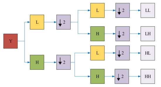
Figure 1.
2D-DWT for one decomposition level [48].
2.3. Explanation of TNN and Optimized based Image De-noising
Wavelet-based image de-noising can be performed as follows [1], [37]. Applying a wavelet transform provides us with the wavelet detail (important or significant) and noisy (non-important) components. It is obvious that the important features of the image need to remain, and the non-important characteristics need to be discarded. Therefore, we can apply a suitable threshold function to do so. The threshold function can easily tune the wavelet components by the threshold value. By applying the threshold function, we will obtain the thresholded wavelet constituents. In order to obtain the output de-noised image, we are required to apply the inverse discrete wavelet transform (IDWT). This de-noising process is shown in Figure 2.
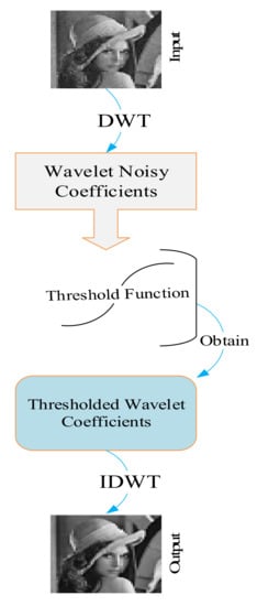
Figure 2.
Wavelet-based image de-noising.
Zhang first proposed noise removal using a thresholding neural network (TNN) in 2001 [37]. Unlike the neural network, in TNN, the linear transform is fixed, and the activation function can be adaptive. In this network, we can get noisy coefficients by applying the linear transform on the noisy input image. Then, these noisy components can be passed through the non-linear activation function to get thresholded wavelet constituents. In the end, the inverse linear transform will be applied to these thresholded coefficients to obtain noise-free images. The improved soft and hard functions proposed by Zhang (2001) [37] are two types of non-linear threshold function which can be used in this network.
where is the improved soft threshold function, is the wavelet component, and is a user-defined function parameter [37].
where is the improved hard threshold function, is the wavelet components, t is the threshold value and is a user-defined function parameter [37].
We can attain the optimum threshold value in the step as follows [39]:
where (S) is defined as:
where is the learning rate, and is the mean square error (MSE) risk function.
Nasri and Nezamabadi-pour in 2009 [40] proposed a sub-band adaptive TNN network with a new non-linear threshold function. In adaptive wavelet-based noise removal techniques, the threshold functions are chosen to be non-linear and adaptive. This function is given below.
where is the wavelet coefficient, a and b are the shape-tuning parameters, and c calculates the asymptote of the function.
Noise removal using TNN with the steepest descent learning is time-consuming. In 2016, Bhandari et al. [41] proposed utilizing the meta-heuristic nature-inspired optimization algorithm (JADE algorithm) instead of using TNN to improve the qualitative and quantitative result and to increase the speed. In 2019, Golilarz et al. [1] improved the quality of the previous method by utilizing the HHO optimizer. It was proven that using the HHO algorithm can increase the speed of processing remarkably. The whole procedure of optimization-based noise reduction is shown in Figure 3.
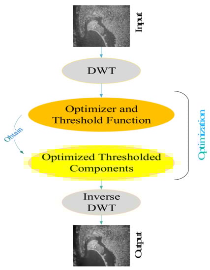
Figure 3.
Optimized-based image de-noising procedure.
3. Proposed Technique
3.1. Explanation of AGGD and Improved AGGD
Although optimization-based noise reduction could solve some drawbacks of utilizing the TNN, the quality of the de-noised image needs to be improved, and the computational time also needs to be decreased. In 2019, an adaptive generalized Gaussian distribution (AGGD)-oriented threshold was proposed for image de-noising [44]. The process of acquiring this data-driven function is formulated below [44]. This procedure is illustrated in Figure 4.
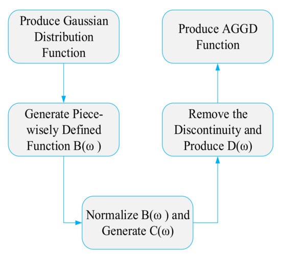
Figure 4.
The process of obtaining AGGD-oriented threshold function.
Step 1: Produce zero-mean Gaussian distribution function as below.
Step 2: Produce B() as follows:
Then, B() can be alternatively formulated as follows.
Step 3: Produce Normalized B():
Step 4: Produce D() as below:
Step 5: Produce AGGD threshold function E():
where E(ω) is the AGGD threshold function, is the wavelet coefficient, is the robust median estimator [45], and is the threshold value, which is the intersection of () and .
To improve the quality of the previous research, Golilarz et al. (2019) [1] presented a complete non-linear function as an improved version of the AGGD threshold function. This function could also improve the processing speed of former AGGD, TNN-based, and optimization-based noise reduction techniques. It is not required to apply the steepest descent learning and optimization algorithms to attain the threshold value [1]. The improved AGGD function is formulated below. Figure 5 depicts both the AGGD and the improved AGGD functions together.
where β (ω) is the improved AGGD threshold function.
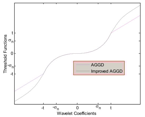
Figure 5.
The AGGD threshold and the improved AGGD threshold (for ) [1].
3.2. Proposed Enhanced AGGD
The improved AGGD threshold function could enhance the qualitative and quantitative results of TNN and optimization-based noise removal. As we mentioned before, the improved AGGD consists of two main parts. In the interval [-t, t], the function is adaptive GGD, and behind the interval, it is a non-linear function. The threshold value is . In this section, an enhanced version of the former improved AGGD threshold is presented. In the proposed technique, . Similar to the improved AGGD, the developed function also contains two parts: in the interval, [], which is adaptive GGD, and behind the interval is non-linear. Note that, unlike the improved AGGD function, there is no intersection between the adaptive GGD and the identity function. Based on the experimental results, this function could improve the performance of the former techniques and also it could provide us with a faster processing time. The proposed function is formulated below. Figure 6 illustrates the enhanced adaptive GGD threshold.
where, () is the proposed enhanced AGGD function, C() , is the coefficient, and .
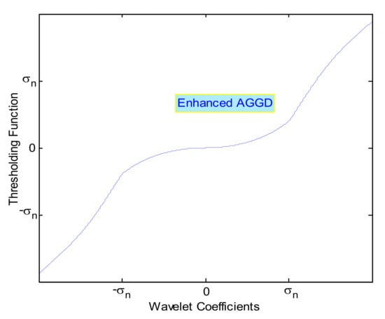
Figure 6.
Enhanced adaptive threshold function for
The proposed enhanced AGGD Algorithm 1 is as follows:
| Algorithm 1: Enhanced AGGD |
Input: Wavelet Coefficients
|
4. Experimental Analysis
Note that in this study, for evaluating the de-noising performance of various methods, we utilized the peak signal-to-noise ratio (PSNR), which is given below:
where is the mean square error, as follows.
where is the original image, is de-noised image, and is the size of the image [41].
In the experimental part, we performed several experiments to analyze the results of the proposed approach. Note that, in all the experiments, the Db4 wavelet with one level of decomposition has been utilized. Besides this, we have used eight original satellite images, as shown in Figure 7. The dataset is available in Ref. [1]. We also utilized four hyperspectral images, namely, Indian Pine (captured by AVIRIS sensor), Washington DC Mall (captured by HYDICE sensor), Pavia Center and Pavia University (captured by ROSIS sensor). The dataset is available in Ref. [47]. For the optimization algorithms used in this section, the swarm size is considered 30 and the maximum iteration 500 [1]. The parameters of the HHO and JADE optimizers are the same as those which have been utilized in Refs. [43] and [41], respectively. Note that in these experiments, additive white Gaussian noise (AWGN) with zero mean and different standard deviations has been used for noisy images. For these implementations, Matlab programming language has been used on a computer with Intel Core i7 and 16 GB Ram.
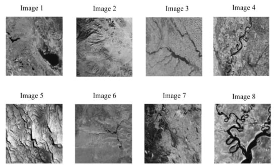
Figure 7.
Test images.
5. Results and Discussions
In the first experiment, as can be seen from Table 1, a comparison has been made between the proposed technique with improved AGGD [1], HHO [1], Bayes [23] and Sure [17] in terms of PSNR values for different standard deviations. The results indicate that the proposed enhanced AGGD performed better than other techniques. Here we have utilized five satellite images.

Table 1.
Comparison of different noise removal methods in terms of PSNR (dB).
Moreover, as we can see from Figure 8, this study compared the proposed technique with other methods visually and qualitatively as well. In this experiment, Image 4 has been used as the test image contaminated by additive white Gaussian noise (AWGN) with zero mean and standard deviation of 30 to obtain the noisy image. Obviously, the visual inspection of the de-noised image obtained by the proposed method is better than the resolution of other approaches.
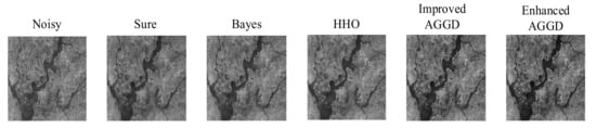
Figure 8.
Visual comparison of different de-noising methods for Image 4.
Furthermore, in this experiment, we compared the enhanced adaptive-based noise reduction method (proposed method) with the improved AGGD [1], HHO-based noise reduction, Bayes [23] and Sure [17] for larger values.
Based on the results in Figure 9, the proposed method gives higher PSNR values for larger standard deviations as compared to other methods. To evaluate the performance analysis of the developed method, MSSIM is also used in the way it is utilized in Ref. [41]. On this correspondence, Figure 10 illustrates the quantitative analysis of several noise reduction methods for larger standard deviations in terms of MSSIM values. As it is evident, the developed method performs promisingly even for large standard deviations. Here we used test Image 3.
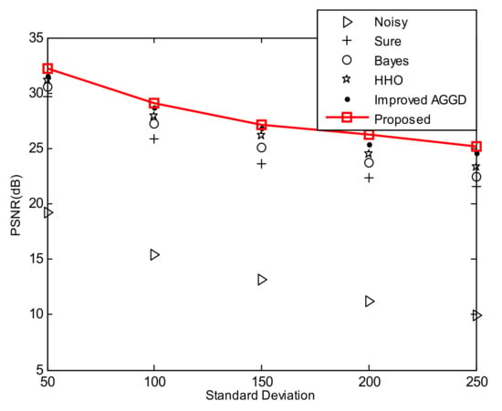
Figure 9.
PSNR comparisons of different de-noising methods for larger values.
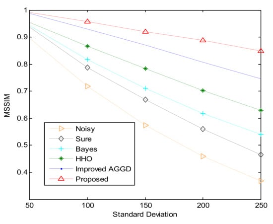
Figure 10.
MSSIM comparisons of different de-noising methods for larger values.
Enhanced AGGD-based noise removal is introduced to improve the quality of the de-noised image. In addition to the quality improvement, the computational cost of the function is cheaper than the alternative methods (improved AGGD [1], HHO [1], Bayes [23], and Sure [17]). We compared the computational time and speed of the processing between different noise reduction methods in Table 2. Test Image 3 has been used in this experiment. The standard deviation is = 10. For all these methods, the time is the average of 20 runs. Obviously, the enhanced adaption-based noise reduction method (developed method) is the fastest technique compared to other techniques.
Table 2.
Comparison of processing time for different methods.
In the second experiment, we made a comparison between the proposed enhanced AGGD-based noise reduction with the soft threshold technique, both qualitatively and quantitatively. Figure 11 shows this comparison. The numbers are PSNR (dB).
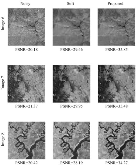
Figure 11.
Comparing between the proposed method and soft thresholding for images 6, 7 and 8 for the standard deviation of 20.
In the third experiment, we used test Image 5 to compare the performance analysis of the proposed enhanced AGGD technique with adaptive soft and adaptive hard [46], and standard soft and standard hard, threshold functions for . As can be seen from Figure 12 the results show that the proposed method outperforms other methods in terms of PSNR value.
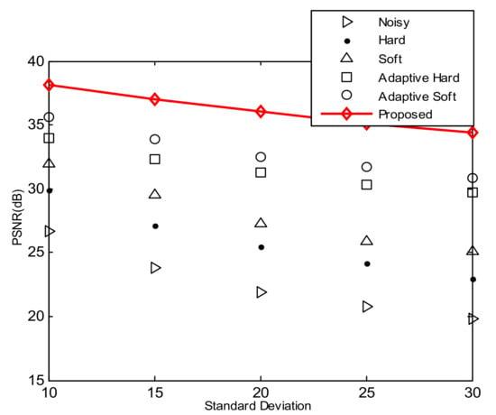
Figure 12.
Quantitative comparison of proposed enhanced AGGD, adaptive threshold and standard threshold functions.
In the fourth experiment, band 20 of the Washington DC Mall (WDM) hyperspectral image [26] is utilized to show that the proposed technique performs well, even in the de-noising of hyperspectral images. For WDM, we considered the same patch which has been used in Ref. [26]. Figure 13 shows the comparison between the proposed enhanced AGGD method and the AGGD [44], JADE [41], and Nasri’s methods [40] for different standard deviations. The results display the superiority of the proposed technique in terms of PSNR values.
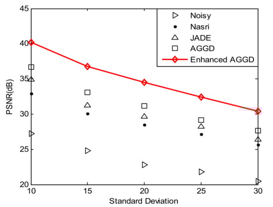
Figure 13.
PSNR results of different techniques for de-noising band 20 of the WDM hyperspectral image.
In the last experiment, to further analyze the performance of the developed method, we used the Indian Pine, Pavia Center and Pavia University hyperspectral images (HSI) to compare the proposed method with some other well-known approaches. The patches of these datasets are utilized in the same way as in Ref. [26]. Noisy images can be acquired by adding AWGN with zero mean and a standard deviation of 10. In Table 3, we compared the de-noising results of the proposed technique with VisuShrink [45], SureShrink [17], BayesShrink [23], and Bivariate shrinkage [22]. The results indicated that the proposed method acts promisingly in de-noising the hyperspectral remote sensing images as well.
Table 3.
Performance analysis of several de-noising methods in terms of PSNR (dB) for different hyperspectral images for the standard deviation of 10.
6. Conclusions
Noise removal utilizing TNN and optimization algorithms can achieve desirable results. However, some existing issues still need to be addressed and solved to improve their qualitative and quantitative results, particularly for light detection and ranging (LiDAR) point clouds [49] and hyperspectral images [50,51]. In wavelet-based image de-noising, the threshold value is very important. This optimum value can be obtained using a least mean square (LMS) learning in the TNN network and using an optimization algorithm in an optimization-based image de-noising approach. These TNN and optimized noise reduction methods perform well but still fail to keep the de-noised image’s visual quality. A new enhanced version of the adaptive generalized Gaussian distribution (AGGD)-oriented threshold function has been introduced in this study to solve this drawback. Utilizing this function can provide us with a cheaper computational cost since we will not apply any LMS learning or optimization algorithms to attain the optimum threshold value. The most important attributes and characteristics of this function are that it is a data-driven and non-linear function. This function consists of two parts. There exists an adaptive GGD function in the interval [−, ] to tune the small noisy coefficients. Moreover, there exists another non-linear function behind the interval [−, ] to tune the larger wavelet components. The results show that the proposed enhanced AGGD-oriented function is a promising method in de-noising the satellite remote sensing images [52,53]. For future work, to achieve better results, we will deal with utilizing some optimization algorithms [54] and also will focus on the non-linear part behind the interval, in which we will use a new type of non-linear data-driven function to be connected to the AGGD function in the interval [−, ].
Author Contributions
Conceptualization, N.A.G. and H.G.; methodology, N.A.G.; software, N.A.G., S.P. and M.Y.; validation, H.G., S.P and J.Z.; formal analysis, Y.F.; investigation, N.A.G. and H.G.; resources, N.A.G., S.P. and H.G.; data curation, N.A.G. and S.P.; writing—original draft preparation, N.A.G., J.Z. and Y.F.; writing—review and editing, N.A.G., H.G., S.P. and M.Y.; visualization, J.Z. and Y.F.; supervision, H.G.; project administration, H.G.; funding acquisition, H.G. All authors have read and agreed to the published version of the manuscript.
Funding
This research was funded by the National Natural Science Foundation of China, Grant No. 61673085.
Data Availability Statement
The data is available upon request for readers and researchers.
Conflicts of Interest
The authors declare no conflict of interest.
References
- Golilarz, N.A.; Gao, H.; Demirel, H. Satellite image De-noising with harris hawks meta heuristic optimization algorithm and improved adaptive generalized Gaussian distribution threshold function. IEEE Access. 2019, 7, 57459–57468. [Google Scholar] [CrossRef]
- Chen, C.L.P.; Liu, L.; Chen, L.; Tang, Y.Y.; Zhou, Y. Weighted couple sparse representation with classified regularization for impulse noise removal. IEEE Trans. Image Process. 2015, 24, 4014–4026. [Google Scholar] [CrossRef] [PubMed]
- Chan, R.H.; Ho, C.W.; Nikolova, M. Salt-and-peppe rnoise removal by median- type noise detectors and detail-preserving regularization. IEEE Trans. Image Process. 2005, 14, 1479–1485. [Google Scholar] [CrossRef] [PubMed]
- Garnett, R.; Huegerich, T.; Chui, C.; He, W. A universal noise removal algorithm with an impulse detector. IEEE Trans. Image Process. 2005, 14, 1747–1754. [Google Scholar] [CrossRef]
- Yin, J.; Chen, B.; Li, Y. Highly accurate image reconstruction for multimodal noise suppression using semisupervised learning on big data. IEEE Trans. Multimed. 2018, 20, 3045–3056. [Google Scholar] [CrossRef]
- De Decker, A.; François, D.; Verleysen, M.; Lee, J.A. Mode estimation in high-dimensional spaces with flat-top kernels: Application to image denoising. Neurocomputing 2011, 74, 1402–1410. [Google Scholar] [CrossRef]
- Portilla, J.; Strela, V.; Wainwright, M.J.; Simoncelli, E.P. Image denoising using scale mixtures of Gaussians in the wavelet domain. IEEE Trans. Image Process. 2003, 12, 1338–1351. [Google Scholar] [CrossRef]
- Miura, S.; Tsuji, H.; Kimura, T. Randomly valued impulse noise removal using Gaussian curvature of image surface. In Proceedings of the IEEE International Symposium on Intelligent Signal Processing and Communication Systems, Naha, Japan, 12–15 November 2013; pp. 291–296. [Google Scholar]
- Lu, X.; Yuan, Y.; Yan, P. Sparse coding for image denoising using spike and slab prior. Neurocomputing 2013, 106, 12–20. [Google Scholar] [CrossRef]
- Yuan, G.; Ghanem, B. LOTV: A new method for image restoration in the presense of impulse noise. In Proceedings of the IEEE Conference on Computer Vision and Pattern Recognition, Boston, MA, USA, 7–12 June 2015; pp. 5369–5377. [Google Scholar]
- Lin, C.H.; Tsai, J.S.; Chiu, C.T. Switching bilateral filter with a texture/noise detector for universal noise removal. IEEE Trans. Image Process. 2010, 19, 2307–2320. [Google Scholar]
- Awad, A.S. Standard deviation for obtaining the optimal direction in the removal of impulse noise. IEEE Signal Process. Lett. 2011, 18, 407–410. [Google Scholar] [CrossRef]
- Dong, Y.; Xu, S. A new directional weighted median filter for removal of random-valued impulse noise. IEEE Signal Process. Lett. 2007, 14, 193–196. [Google Scholar] [CrossRef]
- Lin, T.C. A new adaptive center weighted median filter for suppressing impulsive noise in images. Inf. Sci. 2007, 177, 1073–1087. [Google Scholar] [CrossRef]
- Green, A.A.; Berman, M.; Switzer, P.; Craig, M.D. A Transformation for Ordering Multispectral Data in Terms of Image Quality with Implications for Noise Removal. IEEE Trans. Geosci. Remote Sens. 1988, 26, 65–74. [Google Scholar] [CrossRef]
- Zhang, H. Hyper-spectral Image De-noising with Cubic Total Variation Model. ISPRS Ann. Photogramm. Remote Sens. Spat. Inf. Sci. 2012, 1, 95–98. [Google Scholar] [CrossRef]
- Donoho, D.L.; Johnstone, I.M. Adapting to unknown smoothness via wavelet shrinkage. J. Am. Stat. Assoc. 1995, 90, 1200–1224. [Google Scholar] [CrossRef]
- Chang, S.G.; Yu, B.; Vetterli, M. Spatially adaptive wavelet thresholding with context modeling for image denoising. IEEE Trans. Image Process. 2000, 9, 1522–1531. [Google Scholar] [CrossRef]
- Figueiredo, M.A.; Nowak, R.D. Wavelet-based image estimation: An empirical Bayes approach using Jeffrey’s noninformative prior. IEEE Trans. Image Process. 2001, 10, 1322–1331. [Google Scholar] [CrossRef]
- Achim, A.; Bezerianos, A.; Tsakalides, P. Novel Bayesian multiscale method for speckle removal in medical ultrasound Images. IEEE Trans. Med. Imaging 2001, 20, 772–783. [Google Scholar] [CrossRef]
- Starck, J.L.; Candès, E.J.; Donoho, D.L. The curvelet transform for image denoising. IEEE Trans. Image Process. 2002, 11, 670–684. [Google Scholar] [CrossRef]
- Sendur, L.; Selesnick, I.W. Bivariate shrinkage functions for wavelet-based denoising exploiting interscale dependency. IEEE Trans. Signal Process. 2002, 50, 2744–2756. [Google Scholar] [CrossRef]
- Chang, S.G.; Yu, B.; Vetterli, M. Adaptive Wavelet Thresholding for Image De-noising and Compression. IEEE Trans. Image Process. 2000, 9, 1532–1546. [Google Scholar] [CrossRef] [PubMed]
- Sveinsson, J.R.; Benediktsson, J.A. Almost translation invariant wavelet transformations for speckle reduction of SAR images. IEEE Trans. Geosci. Remote Sens. 2003, 41, 2404–2408. [Google Scholar] [CrossRef]
- Achim, A.; Tsakalides, P.; Bezerianos, A. SAR image denoising via Bayesian wavelet shrinkage based on heavy-tailed modeling. IEEE Trans. Geosci. Remote.Sens. 2003, 41, 1773–1784. [Google Scholar] [CrossRef]
- Golilarz, N.A.; Gao, H.; Ali, W.; Shahid, M. Hyper-spectral remote sensing image de-noising with three dimensional wavelet transform utilizing smooth nonlinear soft thresholding function. In Proceedings of the IEEE 15th International Computer Conference on Wavelet Active Media Technology and Information Processing, Chengdu, China, 14–16 December 2018; pp. 142–146. [Google Scholar]
- Pižurica, A.; Philips, W.; Lemahieu, I.; Acheroy, M. A joint inter- and intrascale statistical model for Bayesian wavelet based image denoising. IEEE Trans. Image Process. 2002, 11, 545–557. [Google Scholar] [CrossRef] [PubMed]
- Golilarz, N.A.; Robert, N.; Addeh, J.; Salehpour, A. Translation Invariant Wavelet Based Noise Reduction Using a New Smooth Nonlinear Improved Thresholding Function. Comput. Res. Prog. Appl. Sci. Eng. 2017, 3, 104–108. [Google Scholar]
- Golilarz, N.A.; Demirel, H. Image de-noising using un-decimated wavelet transform (UWT) with soft thresholding technique. In Proceedings of the IEEE 9th International Conference on Computational Intelligence and Communication Networks, Girne, Cyprus, 16–17 September 2017; pp. 16–19. [Google Scholar]
- Kong, X.; Zhao, Y.; Xue, J.; Cheung-Wai Chan, J.; Ren, Z.; Huang, H.; Zang, J. Hyperspectral image denoising based on nonlocal low-rank and TV regularization. Remote Sens. 2020, 12, 1956. [Google Scholar] [CrossRef]
- Ma, T.; Xu, Z.; Meng, D. Remote sensing image denoising via low-rank tensor approximation and robust noise modeling. Remote Sens. 2020, 12, 1278. [Google Scholar] [CrossRef]
- Elad, M.; Aharon, M. Image denoising via sparse and redundant representations over learned dictionaries. IEEE Trans. Image Process. 2006, 15, 3736–3745. [Google Scholar] [CrossRef]
- Coifman, R.R.; Donoho, D.L. Translation-invariant de-noising. In Wavelets and Statistics; Springer: New York, NY, USA, 1995; Volume 103, pp. 125–150. [Google Scholar]
- Golilarz, N.A.; Demirel, H. Thresholding neural network (TNN) with smooth sigmoid based shrinkage (SSBS) function for image de-noising. In Proceedings of the IEEE 9th International Conference on Computational Intelligence and Communication Networks, Girne, Cyprus, 16–17 September 2017; pp. 67–71. [Google Scholar]
- Dan, L.; Yan, W.; Ting, F. Wavelet image denoising algorithm based on local adaptive wiener filtering. In Proceedings of the IEEE International Conference on Mechatronic Science, Electric Engineering and Computer MEC, Jilin, China, 19–22 August 2011; pp. 2305–2307. [Google Scholar]
- Golilarz, N.A.; Demirel, H. Thresholding neural network (TNN) based noise reduction with a new improved thresholding function. Comput. Res. Prog. Appl. Sci. Eng. 2017, 3, 81–84. [Google Scholar]
- Zhang, X.P. Thresholding neural network for adaptive noise reduction. IEEE Trans. Neural Netw. 2001, 12, 567–584. [Google Scholar] [CrossRef]
- Qian, Y. Image de-noising algorithm based on improved wavelet threshold function and median filter. In Proceedings of the IEEE 18th International Conference on Communication Technology, Chongqing, China, 8–11 October 2018; pp. 1197–1202. [Google Scholar]
- Sahraeian, S.M.E.; Marvasti, F.; Sadati, N. Wavelet image denoising based on improved thresholding neural network and cycle spinning. In Proceedings of the IEEE International Conference on Acoustics, Speech and Signal Processing, Honolulu, HI, USA, 15–20 April 2007; pp. 585–588. [Google Scholar]
- Nasri, M.; Nezamabadi-pour, H. Image denoising in the wavelet domain using a new adaptive thresholding function. Neurocomputing 2009, 72, 1012–1025. [Google Scholar] [CrossRef]
- Bhandari, A.K.; Kumar, D.; Kumar, A.; Singh, G.K. Optimal sub-band adaptive thresholding based edge preserved satellite image denoising using adaptive differential evolution algorithm. Neurocomputing 2016, 174, 698–721. [Google Scholar] [CrossRef]
- Zhang, J.; Sanderson, A.C. JADE: Adaptive differential evolution with optional external archive. IEEE Trans. Evol. Comput. 2009, 13, 945–958. [Google Scholar] [CrossRef]
- Heidari, A.A.; Mirjalili, S.; Faris, H.; Aljarah, I.; Mafarja, M.; Chen, H. Harris hawks optimization: Algorithm and applications. Future Gener. Comput. Syst. 2019, 97, 849–872. [Google Scholar] [CrossRef]
- Golilarz, N.A.; Demirel, H.; Gao, H. Adaptive generalized Gaussian distribution oriented thresholding function for image de-noising. Int. J. Adv. Comput. Sci. Appl. 2019, 10, 10–15. [Google Scholar] [CrossRef]
- Donoho, D.L.; Johnstone, I.M. Ideal Spatial Adaptation by Wavelet Shrinkage. Biometrika 1993, 81, 425–455. [Google Scholar] [CrossRef]
- Golilarz, N.A.; Gao, H.; Kumar, R.; Ali, L.; Fu, Y.; Li, C. Adaptive wavelet based MRI brain image de-noising. Front. Neurosci. 2020, 14, 728. [Google Scholar] [CrossRef]
- Rasti, B.; Sveinsson, J.R.; Ulfarsson, M.O.; Benediktsson, J.A. Hyper-spectral Image De-noising Using 3D Wavelets. In Proceedings of the IEEE International Geoscience and Remote Sensing Symposium, Munich, Germany, 22–27 July 2012; pp. 1349–1352. [Google Scholar]
- Lei, L.; Wang, C.; Liu, X. Discrete Wavelet Transform Decomposition Level Determination Exploiting Sparseness Measurement. Int. J. Electr. Comput. Energetic Electron. Commun. Eng. 2013, 7. [Google Scholar]
- Pirasteh, S.; Rashidi, P.; Rastiveis, H.; Huang, S.; Zhu, Q.; Liu, G.; Li, Y.; Li, J.; Seydipour, E. Developing an Algorithm for Buildings Extractions and Determining Changes from Airborne LiDAR Point Clouds. Remote Sens. 2019, 11, 1272. [Google Scholar] [CrossRef]
- Li, Z.; Li, J.; Zhou, S.; Pirasteh, S. Developing an Algorithm for Local Anomaly Detection based on Spectral Space Window in Hyperspectral Image. Earth Sci. Inform. 2015, 8, 741–749. [Google Scholar] [CrossRef]
- Li, Z.; Li, J.; Zhou, S.; Pirasteh, S. Comparison of spectral and spatial windows for local anomaly detection in hyperspectral imagery. Int. J. Remote Sens. 2015, 36, 1570–1583. [Google Scholar] [CrossRef]
- Mao, W.; Liu, G.; Wang, X.; Xiang, W.; Wu, S.; Zhang, B.; Bao, J.; Cai, J.; Zhang, R.; Pirasteh, S. Combining Azimuth Offset-based and RSS Methods Based on Variance Component Estimation for InSAR Ionospheric Correction. IEEE J. Sel. Top. Appl. Earth Obs. Remote Sens. 2020. [Google Scholar] [CrossRef]
- Pirasteh, S.; Safari, H.O. Digital Processing of SAR Data and Image Analysis Techniques, Monitoring and Modeling of Global Changes: A Geomatics Perspective. In Monitoring and Modeling of Global Changes: A Geomatics Perspective; Springer: Dordrecht, The Netherlands, 2015; pp. 281–301. [Google Scholar] [CrossRef]
- Golilarz, N.A.; Gao, H.; Addeh, A.; Pirasteh, S. Orca Optimization Algorithm: A New Meta-Heuristic Tool for Complex Optimization Problems. In Proceedings of the 17th ICCWAMTIP, Chengdu, China, 18 December 2020. [Google Scholar]


Publisher’s Note: MDPI stays neutral with regard to jurisdictional claims in published maps and institutional affiliations. |
© 2020 by the authors. Licensee MDPI, Basel, Switzerland. This article is an open access article distributed under the terms and conditions of the Creative Commons Attribution (CC BY) license (http://creativecommons.org/licenses/by/4.0/).