Abstract
Gaps are important for growth of vegetation on the forest floor. However, monitoring of gaps in large areas is difficult. Airborne light detection and ranging (LiDAR) data make precise gap mapping possible. We formulated a method to describe changes in gaps by time-series tracking of gap area changes using three digital canopy height models (DCHMs) based on LiDAR data collected in 2005, 2011, and 2016 over secondary deciduous broadleaf forest. We generated a mask that covered merging or splitting of gaps in the three DCHMs and allowed us to identify their spatiotemporal relationships. One-fifth of gaps merged with adjacent gaps or split into several gaps between 2005 and 2016. Gap shrinkage showed a strong linear correlation with gap area in 2005, via lateral growth of gap-edge trees between 2005 and 2016, as modeled by a linear regression analysis. New gaps that emerged between 2005 and 2011 shrank faster than gaps present in 2005. A statistical model to predict gap lifespan was developed and gap lifespan was mapped using data from 2005 and 2016. Predicted gap lifespan decreased greatly due to shrinkage and splitting of gaps between 2005 and 2016.
1. Introduction
A forest canopy gap (hereafter, gap) is an open area formed in the upper forest canopy. Gaps are formed when one or more trees are lost to typhoon damage, damage by insects and diseases, felling, or other causes of tree mortality. In closed-canopy forests, gap environments differ greatly from the surrounding forest floor. Because gap formation improves the light environment on the forest floor and advances growth of understory vegetation, which is suppressed under closed canopies, gaps play an important role in forest regeneration. Gap dynamics, from gap formation to sapling regeneration, differ among forest ecosystems, and influence forest structure and biodiversity [1]. Therefore, an understanding of gap dynamics is important for adaptive management, which involves simultaneously managing and learning about forest ecosystems while monitoring forest status, evaluating biodiversity, planning long-term resource utilization, and preserving or remodeling the landscape [2].
Forest regeneration following disturbances such as gap formation is classified into four major patterns: sprout regeneration from stumps, advance regeneration by seedlings in the understory, regeneration by buried seeds, and regeneration from seeds dispersed after the disturbance [3]. In addition, a disturbed area can be closed by growth of the surrounding trees [4]. The regeneration pattern depends on gap size and the environment surrounding the gap [5]. Gap regeneration has been studied via field gap surveys that measured the undergrowth height distribution [6], regeneration by tree species [7], differences in gap size and seedling species in different regeneration stages [8], and the relationship between gap size and light intensity on the forest floor [9]. These works make clear substitution of the tree species in gaps, shade-tolerance, and height growth of tree species which participate in the regeneration in gaps. However, because it is difficult to measure and re-measure the spatial distribution of gaps accurately by ground surveys, few studies have investigated the changes in numerous gaps over long periods of time [10,11].
Recent progress in survey technologies such as aerial photography and airborne light detection and ranging (LiDAR) has enabled collection of spatial information over large areas of forest, which cannot be obtained by ground surveys [12,13]. Since gap monitoring is important for understanding forest dynamics, forest canopies were previously monitored using time-series canopy height models created by using aerial photos between 1/10,000 and 1/20,000 in scale [14,15,16,17]. Digital surface models (DSMs), which use elevation data to represent the earth’s surface, including objects such as buildings or trees, can be obtained by image-to-image matching of aerial photos. However, the coarse-resolution DSMs obtained by image matching cannot reveal details of crown cover. In order to perform fine-scale gap monitoring, including small gaps caused by the fall or damage of single trees, it is necessary to obtain detailed data on the structure of the forest canopy. LiDAR data can be used to provide precise geolocations of gaps and to describe forest canopies in detail, permitting monitoring of gap dynamics over wide areas [18,19].
Optical sensors, synthetic aperture radars (SARs), and LiDARs are commonly used for canopy parameter estimation of forest [20]. Optical sensors receive reflected solar radiation and emitted radiation from surface as spectral radiance and SARs emit microwave energy and receive energy scattered back (backscatter) from forest. Canopy parameters such as tree height or biomass are estimated indirectly by analyzing their relationship with radiance [21,22] or backscatter signal [23,24]. Indirect estimation makes precise canopy parameter estimation difficult.
On the other hand, LiDAR instruments measure distance to and reflected pulse intensity from ground objects by laser measurement, and they can provide precise three-dimensional location data when combined with global positioning system (GPS) and inertial measurement unit (IMU) data [25]. LiDAR data have been widely used for forest analyses since the late 1990s, and some datasets have become available. Detailed, wide-ranging forest analysis using LiDAR data has revealed detail forest status that could not be revealed by field surveys or aerial photo analysis [26,27,28]. Like DSMs, digital terrain models (DTMs), which show ground surface elevation without objects or trees, are derived from LiDAR data. Using the differences between DSMs and DTMs, the height of tree crowns can be determined in order to create digital canopy height models (DCHMs) [29].
Researchers have used DCHMs to analyze the relationship between tree height and topography [30], estimate stem volume [31,32,33,34,35,36,37], and classify conifer species by crown shape [38,39,40,41]. Gap detection [42] and gap monitoring [43] have been carried out over large areas, and a series of studies have used time-series LiDAR data to elucidate gap expansion, gap closure, species regeneration, and gap spatial dynamics in a Canadian boreal forest [18,26,27,28].
Here, using LiDAR data collected at three different times over a cool temperate deciduous broadleaf forest in Japan, we focused on gap shrinkage and expansion, with the following three objectives. First, we tracked changes in gaps such as size, merging, and splitting, thereby showing the effectiveness of LiDAR data for monitoring gaps over a large area. Second, we analyzed the relationship between initial gap area and gap shrinkage over 11 years. Third, we predicted the time to gap closure (gap lifespan) based on the rate of gap shrinkage.
2. Materials and Methods
2.1. Study Site
Our study site was set in deciduous secondary broadleaf forest (centered at 137°25.5′E, 36°9′N, 3.4 × 1.6 km, 1.74 km2, Figure 1) in the upper valley of the Namai River near Takayama, Gifu, central Japan (Figure 1). The topography is rather steep, mostly with slopes between 30° and 40°, and elevation ranging between ca. 1080 m and ca. 1490 m above sea level (ASL). The deciduous broadleaf forest is surrounded by coniferous forest plantations composed of Japanese cedar (Cryptomeria japonica), Hinoki cypress (Chamaecyparis obtusa), and Japanese larch (Larix leptolepis). The deciduous secondary broadleaf forest is mainly composed of Mongolian oak (Quercus mongolica var. grosseserrata), Japanese umbrella tree (Magnolia obovata), and birch (Betula spp.). Bamboo grass spp. (Sasa spp.), saplings, and young deciduous broadleaf trees and saplings such as Hydrangea paniculata, cherry spp. (Prunus spp.), Japanese linden (Tilia Japonica), maple spp. (Acer spp.), Japanese umbrella tree, birch spp. and Mongolian oak grow in the understory. Height of bamboo grass is between 0.5 m and 2 m. The tree species other than Hydrangea paniculata reach height of the upper canopy layer higher than 5m above ground. This secondary forest was used for harvesting firewood until the 1950s, as indicated by remnants of charcoal kilns, tree size after coppicing, testimony from a long-time resident, and visual interpretation of aerial photos in 1963 obtained from the Forestry Agency of Japan. We executed field surveys in 15 plots between 2010 and 2012, and the average tree height was between 8.5 m and 17.9 m at that time. This study site had been damaged by natural disasters. Many trees were felled by severe winds caused by a typhoon in 2004 [44], and a heavy snowfall in 2014 caused considerable damage to many trees and branches [45]. The site also contains several built objects such as forest roads, some buildings, and ski slopes adjoining or within the broadleaf deciduous forest.
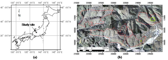
Figure 1.
Study site. (a) Location in Japan; (b) Locations within the deciduous broadleaf forest. The red polygons show the broadleaf forest and the yellow polygon shows the location of an unmanned aerial vehicle (UAV) flight area. The lime square shows the area of gap lifespan prediction maps in Section 3.4. (Background: an aerial ortho-photo captured in October 2016).
2.2. Data
2.2.1. LiDAR Data
LiDAR data collected in 2005, 2011 by Gifu University, and 2016 by the Gifu Prefecture Government were used (Table 1). To generate DSMs, point clouds of geographical locations from July 2005 (LiDAR-2005), August 2011 (LiDAR-2011), and October 2016 (LiDAR-2016) were used. The average pulse densities were 1.54, 4.84, and 5.91 (points m−2) and the standard deviations (SDs) were 1.05, 3.08, and 1.64 (points m−2) in the LiDAR-2005, LiDAR-2011, and LiDAR-2016 datasets, respectively. Pulse density varied with location, and the LiDAR-2011 data, captured by a helicopter-borne platform instead of a fixed-wing platform, showed the highest SD. Areas with high-density pulses were unevenly distributed due to unstable helicopter attitude during the flight, resulting in many small linear overlaps of scan lines in the LiDAR-2011 dataset. A DTM in 0.5 m square mesh (DTM-2016), which was generated from the LiDAR-2016 data by the contractor (Table 1), was also obtained from the Gifu Prefecture Government.

Table 1.
Summary of light detection and ranging (LiDAR) observations.
2.2.2. Aerial Photos Taken by Unmanned Aerial Vehicle (UAV)
Since the 2016 LiDAR data were collected in late October, the deciduous trees might have already begun to lose their leaves. In order to confirm the effects of defoliation, aerial photos were taken over a gap in the southeast part of the study site at ca. 1430 m ASL) on August 30, 2018 from a UAV (Phantom4 Pro, DJI, Shenzhen, China). The UAV flew at 30 m above the takeoff site at 2–5 km/h, taking photos at 2-s intervals. A total of 595 photographs were taken over the total area (1800 m2), and ≥9 photos covered over each gap area. Before the aerial photos were taken, a surveying pole (6 m high) with a survey marker at the tip was placed near the center of the gap as a ground control point (GCP). A DSM (DSM-UAV) and an ortho-photo were generated from the 595 aerial photos using PhotoScan Professional ver. 1.4.3 (Agisoft, Saint Petersburg, Russia).
The GCP was used to calibrate the horizontal coordinates of the DSM-UAV to the DSM generated from the LiDAR-2016 data (DSM-2016). The vertical difference was adjusted using the altitude of the GCP, which was estimated from the ground elevation in the DTM, pole height, and the elevation at the GCP tip in the DSM-UAV using Imagine 2015 (ERDAS Inc., Norcross, GA, USA). Shapes of tree canopies and gaps in the DSM-UAV and DSM-2016 were visually compared.
2.2.3. Forest Type Maps and Aerial Photos
Forest types were identified by using a forest type map [46] with a 2-m grid resolution. Color aerial ortho-photographs with 0.5-m grid resolution taken in 2003, 2011, and 2016 were used to verify gaps and to differentiate artificial objects such as roads from gaps. The 2011 and 2016 aerial ortho-photographs were taken in conjunction with the LiDAR observations. All of the remote sensing data are projected onto the Japanese plane rectangular coordinate system, zone 7 [47].
2.3. Field Survey and Data Processing
Figure 2 shows a flowchart of the analysis procedure, which consisted of four parts: (1) generating DSMs and DCHMs from the LiDAR data; (2) validating the compatibility of the generated DSMs; (3) time-series tracking of gap generation and canopy closure; and (4) modeling gap area reduction.
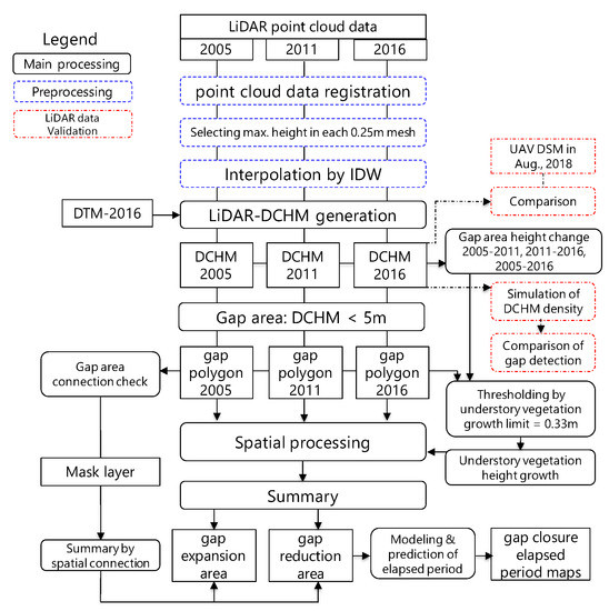
Figure 2.
Analysis flow.
2.3.1. Generating DCHMs and Extracting Gaps from LiDAR Data
Prior to performing the gap analysis, we checked the registration of the three sets of LiDAR data. We selected LiDAR-2016 as the geolocation standard. One-meter-mesh DSM images of the three LiDAR datasets were produced using nearest neighbor resampling [48] for geolocation validation. We compared the geolocations of the four sides of several square buildings on the three DSM images to evaluate the horizontal error. We selected points in flat areas, such as in the center of paved roads or parking areas, that showed no changes over the 11 years to evaluate differences in elevation. The LiDAR-2005 and LiDAR-2011 data stacked accurately on the LiDAR-2016 in the X and Y directions. In the Z direction (elevation), the LiDAR-2005 and LiDAR-2011 data were shifted −0.06 m and −0.04 m relative to the LiDAR-2016 data, respectively; the differences were corrected in the subsequent analysis.
When LiDAR point clouds are rasterized, pulses reflected inside the canopy might be rendered as false gaps. To avoid this, the three LiDAR datasets were divided into 0.25-m mesh, and the pulse with the highest elevation within each mesh was chosen. Its geographical coordinates and altitude were recorded. This procedure was carried out using our in-house system programmed in FORTRAN.
The recorded data were interpolated and rasterized using the inverse distance weighted (IDW) method [18,49], and DSMs at 0.25-m mesh were generated. This procedure was carried out using ArcGIS ver. 10.6 (ESRI, Redlands, CA, USA). The following IDW formulae were used:
where d(x, xi) is the distance between the center of the target mesh x and a DSM point location xi, and p is a parameter that adjusts the influence of distance and controls the influence of the elevation of surrounding point clouds; in this case, p was set at 3. The IDW estimates the value u(x) at the target coordinates or the center of a mesh by interpolation using the closest N elevation datum, u(xi) (i = 0, 1, N) to the target. We set the number of samples (N) as 12, the default in the IDW tool. Sometimes a mesh did not include LiDAR point clouds, especially in LiDAR-2005 and LiDAR-2011, because of low or variable pulse density (Table 1). The elevation of the closest point to those blank meshes had the greatest influence on the interpolation.
For alignment with the resolution of the DSMs, DTM-2016 was interpolated from a 0.5-m mesh to a 0.25-m mesh by bi-linear interpolation [48] using Imagine 2015. The DTM was subtracted from each DSM to generate DCHMs with 0.25-m square meshes for each year.
We set the gap height threshold at 5 m after checking the DCHMs and taking into account the average tree height in the 15 plots between 2010 and 2012. As described previously, bamboo grass and young deciduous broadleaf trees such as Mongolian oak, birch spp., cherry spp., and maple spp. grow in the understory, less than 5 m in DCHMs. We analyzed gap size distribution and changes of gaps by expansion of surrounding trees and height growth of understory vegetation in gaps. Based on the DCHMs, gaps and closure of the canopy for each year were detected using ArcGIS 10.6. Values ≥5 m were identified as closed canopy; meshes with values < 5 m were identified as open canopy. Canopy openings were converted to polygons as vector data, and the area surrounding the opening was searched in eight directions, and any adjacent canopy openings were combined with the central mesh. The area of each canopy opening was calculated, and if it was ≥5 m2, the canopy opening polygon was left as a gap and the other was removed. By definition, artificial open spaces such as roads and ski slopes were identified as gaps. Therefore, canopy gaps connected to artificial open spaces identified by visual interpretation of aerial photos were also removed.
2.3.2. Compatibility Validation of Generated DSMs
A DSM-UAV was generated from the aerial photos taken by the UAV, and photos were ortho-rectified. The geometric horizontal coordinates of the DSM-UAV were adjusted to the 2016 DSM using ground objects such as tree tops. The elevation of the DSM-UAV was adjusted to the 2016 DSM using the elevation of the GCP tip. Closed canopy and gaps generated from DSM-UAV and DSM-2016 were compared, to verify the influence of autumnal defoliation.
In order to verify differences in gap extraction from the three LiDAR datasets with different pulse densities, we resampled the DSM generated using the point cloud from LiDAR-2016 to the density of LiDAR-2005 and 2011 (Table 1) randomly over the DSM-UAV coverage (Figure 1). Canopy openings were extracted using the simulated mesh DSMs, and the area and gap overlap (openings ≥ 5 m2) between the two simulated DSMs and the DSM-2016 were calculated.
2.3.3. Time-Series Tracking of Gap Generation and Canopy Closure
The process of gap formation, expansion, shrinkage, and closure is not always completed within a single gap. Some canopy gaps split or merge, and the resulting gaps should be regarded as a single group. The mask for one group covers the entire area of interacting gaps in all observations. The polygons of these gaps in 2005, 2011, and 2016 were united into one polygon with attributes such as observation year and gap area in each observation. Gaps without intersections with other gaps were grouped as single-unit gaps. Gaps with mutual intersections in any observations were combined into a single polygon, a gap mask.
Changes in gap area (shrinkage and expansion) and the height of understory vegetation in gaps were observed between July 2005–August 2011 (period A), August 2011–October 2016 (period B), and 2005–2016 (period C). The amount of change was recomputed using the gap mask. The area of change is the sum of the shrinkage and expansion of a gap when gap polygons from two observations are overlaid (Figure 3). Height change where the DCHMs were <5 m was regarded as a change in understory vegetation height in gap polygons. Growth of understory vegetation in each mesh was identified by a threshold, set as 0.33 m·year−1, based on changes in understory height observed by visual inspection of the three DCHMs.
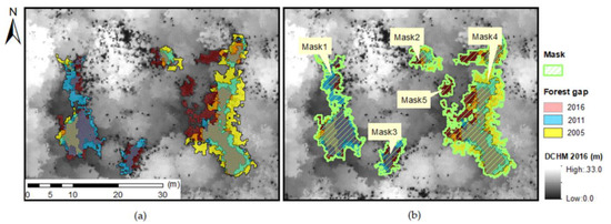
Figure 3.
Gap mask showing gap interactions between 2005 and 2016. (a) Gap overlap between the three digital canopy height models; (b) masks covering interacting gaps.
Gap changes were sorted into the following five categories: “gap formation,” “gap closure,” “gap expansion,” “gap shrinkage by lateral growth of edge trees,” and “gap shrinkage by increased height of understory vegetation” in periods A, B, and C. Gap expansion is the sum of new gaps and expansion of existing gaps.
2.3.4. Modeling Gap Reduction and Lifespan
Focusing on tree crown lateral expansion, models that estimate duration until closure (defined as gap lifespan) based on the relationship between initial gap area and gap shrinkage in a given period were created by a simple regression analysis using JMP 11 (SAS, Cary, NC, USA).
The minimum gap area was defined as 5 m2, and when a gap closes completely, the initial gap area is equal to the gap shrinkage. This suggests that a regression line through the origin would describe the relationship between the initial gap area and gap shrinkage. For this reason, we used the following formula to express the relationship between them.
where A0 is the initial gap area, ΔA0 is the shrinkage of the initial gap k years later (the duration of period L between two LiDAR observations), and a is the slope of the regression line showing shrinkage rate over k years. The general formula that expresses gap shrinkage in k years was derived from Equation (3). The gap area from period 1 to period m using a recurrence Equation of (3) is shown as follows:
ΔA0 = a × A0
Gap area at one period after period L.
AL1 = A0 −ΔA0 = A0 − a × A0 = A0 × (1 − a)
Gap area at two periods after period L.
AL2 = AL1 −ΔAL1 = AL1 − a × AL1 = AL1 × (1 − a) = A0 × (1 − a) × (1 − a) = A0 × (1 − a)2
Gap area at period m after period L.
ALm = A0 × (1 − a)m
A gap area reduction model n years later is expressed as follows from Equation (6).
where An is the gap area (m2) after n years, A0 is the initial gap area (m2), a is the slope in formula (3), and n is elapsed time (years).
An = A0 × (1 − a)n/k
We predicted the years elapsed until gap closure (gap lifespan) using the gap area maps from 2005 and 2016, and produced maps of gap lifespan using Imagine 2015, model (7) and the regression coefficients of the models which were created using JMP 11 in Section 3.4. Differences in gap lifespan predicted by the 2005 and 2016 maps were examined.
Scatter charts and histograms were drawn using Kaleida Graph 4.5 (Synergy Software, Reading, PA, USA) and Delta Graph 7.5 (Nihon Poladigital, Tokyo, Japan), respectively in the analysis.
3. Results
3.1. Generating DCHMs and Extracting Gaps from LiDAR Data
Number of canopy openings in each area class was significantly different (p < 0.001) among the three LiDAR data. The majority of canopy openings extracted from the three LiDAR-DSMs were <1 m2, and the number of gaps of this size in LiDAR-2011 was almost twice that in LiDAR-2005 and LiDAR-2016. However, the number of canopy openings ≥ 1 m2 and <5 m2 was approximately proportional to the average pulse density, in the order LiDAR-2016 ≤ LiDAR-2011 < LiDAR-2005 (Table 2). The number of gaps ≥ 5 m2 did not correspond to the average pulse density, but increased in the order LiDAR-2011 < LiDAR-2016 < LiDAR-2005. Although numerous tiny openings were extracted from LiDAR-2011, this dataset showed the smallest number of gaps among the three LiDAR DSMs. If mesh size is changed to 1.25 m, 99.5% of meshes include at least one pulse. The mesh area is ca. 1.6 m2 and detection error would occur up to about 1.6 m2 and it appeared in Table 2. Number of detected canopy openings < 1 m2 was almost twice of 2005, however, number of detected openings ≥ 1 m2 was the same level with 2016.
Table 2.
Number of canopy openings.
3.2. Compatibility Validation of Generated DSMs
We compared the DSM-UAV (Figure 4c) and DSM-2016 (Figure 4a) images. Because the DSM-2016 has a coarser mesh size, it does not show as detailed a canopy shape as the DSM-UAV. Despite this, the DSM-2016 showed not only branches at the edges of gaps and canopy topography, but also clearly showed the canopy shape of understory trees. Although the LiDAR-2016 data were collected in the middle of autumnal coloring in 2016, it showed the same tree canopy shape as the DSM-UAV data collected in midsummer. We extracted meshes in which canopy height was <5 m from the DSM-2016 and DSM-UAV images, but could not discern any vestiges of fallen leaves in the DSM-2016 image.
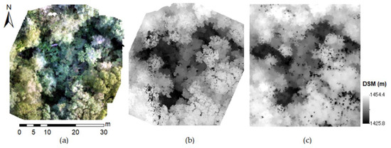
Figure 4.
Comparison of digital surface models (DSMs) produced by unmanned aerial vehicle (UAV) photos and LiDAR-2016. (a) Aerial ortho-photo captured by UAV in Aug. 2018; (b) DSM based on the UAV aerial photos; (c) DSM based on LiDAR-2016 data.
Table 1 shows the average pulse density of the LiDAR-2005, LiDAR-2011, and LiDAR-2016 DSMs in the validation site, which increased in the order 2005 < 2011 < 2016. The pulse density of LiDAR-2005 and LiDAR-2011 was 26.0% and 81.7%, respectively, of that of LiDAR-2016, and we randomly resampled these pulse percentages from LiDAR-2016 to simulate the coverage of LiDAR-2005 and LiDAR 2011 over the coverage of the DSM-UAV. We examined the gap extraction performance with pulse density of LiDAR-2005 and LiDAR-2011. Gap areas extracted from the LiDAR-2016 data had 88.4% and 96.1% overlap with those from the simulated LiDAR-2005 and LiDAR-2011 data, respectively.
3.3. Time-Series Tracking of Gap Generation and Canopy Closure
The gap polygons which were aggregated to single polygons in the connection analysis were classified into the following two types. The first type was gaps that split into several parts. This was observed in many large gaps with complicated shapes. Gaps that split in this way were treated as a single gap polygon by combining the gaps as before the split. The second type was adjacent gaps that merged. This was observed in many stands with many gaps in the study area. The merged gaps were treated as a single gap. However, any gaps that merged with gaps outside the study area (Figure 1b) or artificially open spaces such as forest roads, were removed from the analysis as errors. Re-measurement using the gap mask layer thus increased the maximum, average, median, and SD of the gap area; however, the total gap area was decreased by removal of the gaps that merged with artificial open areas (Table 3).
Table 3.
Summary of gaps.
The number of gaps in each gap class was similar among the three observations (Figure 5). Although the number of gaps in the class <50 m2 ranged from 546 to 787, the overall gap proportions were almost identical. Larger gaps were fewer, and the proportion of gaps in the class ≥100 m2 was <10% in all three LiDAR datasets. This result suggested that formation of gaps of this size is rare in the young to mature secondary deciduous broadleaf forest at the study site.
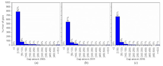
Figure 5.
Number of gaps by area class. (a) Gaps in 2005; (b) gaps in 2011; (c) gaps in 2016.
Changes in gaps over each of the three periods are summarized in Table 4. Number of gaps changed significantly (p < 0.001) between period A and period B in all gap types. First, gap formation was 1.7 times greater, and total gap area was 1.9 times greater in period B than in period A. Thus, gap formation in period B exceeded that in period A, although period B was one year shorter. There were many new gaps < 20 m2 in period B, but only three new gaps ≥ 100 m2 appeared (Figure 6). On the other hand, the number of gaps that closed was 2.0 times higher, and total area of gap closure was 2.3 times higher in period A than in period B. Thus, gap closure in period A also far exceeded that in period B. Although many gaps < 30 m2 closed during period A, the number of gaps ≥ 30 m2 that closed was similar in periods A and B (Figure 7). Differences in average area and minimum area between periods A and B were small for all gap categories. However, the maximum area in the categories “gap formation,” “gap expansion,” and “gap reduction” differed greatly between periods A and B (Table 4). The maximum area of new gaps and expanded gaps reflects the scale of disturbance in the forest, and the SD indicates the maximum area, because a greater change in SD suggests disturbances in many gaps. In period C, which includes periods A and B, the maximum area, the average area, and the SD of each category exceeded those in periods A and B, and gap merging influenced the gap size in period C. Thus, summarizing changes in gap size over periods A and B using the gap mask revealed the dynamics of gap expansion and reduction.
Table 4.
Change of gaps over the periods.
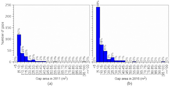
Figure 6.
Number of gaps. New gaps by area class (a) between 2005 and 2011 (period A) and (b) between 2011 and 2016 (period B).
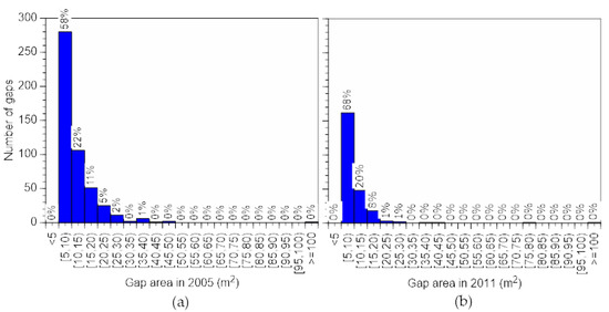
Figure 7.
Number of gap closures by area class. Gap closures (a) between 2005 and 2011 (period A) and (b) between 2011 and 2016 (period B).
The average height increase of understory vegetation per mesh was 0.153 (m year−1), 0.146 (m year−1), and 0.156 (m year−1) in gap opening sections of gaps in periods A, B, and C, respectively, with only small differences between the three periods. We sampled 821 meshes with an annual height increase <0.33 m, set as the upper annual growth limit of understory vegetation. Understory vegetation height increase per mesh had a peak at ~0.18 m year−1 and an SD of 0.048 m year−1 with a balanced bell-shaped distribution (not shown). This suggested that a threshold value of 0.33 m year−1 was appropriate to differentiate height increase of understory vegetation in gap centers from lateral growth of trees at gap edges.
We divided the gaps extracted from the LiDAR-2005 data into four area classes, and summarized the height increment of understory vegetation in period A (Table 5). The average height increment was smallest in the <15 m2 class, and greatest in the class between ≥50 and <100 m2.
Table 5.
Growth of understory vegetation.
We analyzed continuance of gaps present in 2005 through period C (Figure 8a,b). Number of gaps decreased between 2005 and 2011, so that gap number in 2011 was only ca. 0.2 time of that in 2005 (Figure 8b). In 2016, the number of gaps in the ≥5 and >10 m2 class was ca. 0.09 time of that in 2011 (Figure 8c). On the other hand, the number of gaps ≥ 60 m2 was almost identical in 2011 and 2016.
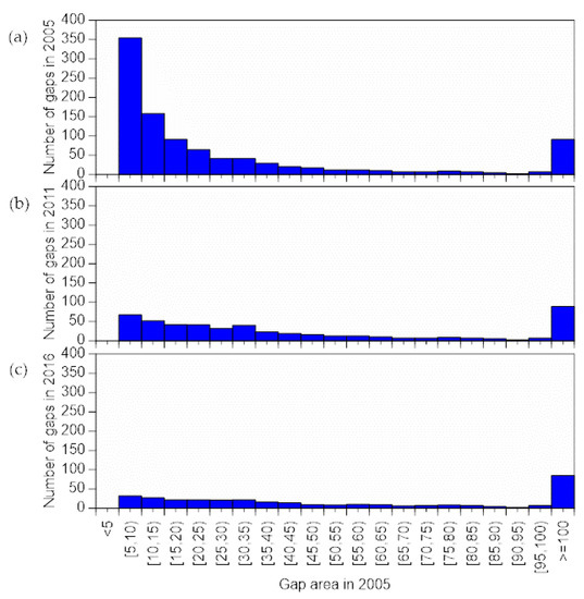
Figure 8.
Changes in number of gaps existed in 2005. (a) Numbers in 2005, (b) 2011, and (c) 2016.
Gap shrinkage is caused by height increase of understory vegetation which are young deciduous broadleaf trees in gaps and by lateral growth of surrounding trees. We analyzed how gap shrinkage caused by each of these factors affected the gap area (GAP2005, m2) (Figure 9). The regression line for growth of understory vegetation (Lc, m2) relative to GAP2005 was as follows:
Lc = 0.0808 × GAP2005
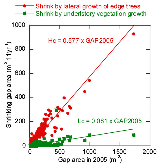
Figure 9.
Relationship between the initial gap area in 2005 and closure or reduction of gap area by 2016. The causes of gap closure are lateral growth of surrounding trees and height increase of understory vegetation. Lateral growth of surrounding trees affected gap closure more strongly than height increase of understory vegetation. The gap area reduction or closure is proportional to the initial gap area.
The coefficient of determination was 0.472 (p < 0.001). The regression line for lateral growth area (Hc, m2) relative to GAP2005 was as follows:
Hc = 0.577 × GAP2005
The coefficient of determination was 0.907 (p < 0.001).
3.4. Modeling of Gap Reduction and Predicting Gap Lifespan
Before investigating the relationship between initial area and gap shrinkage, gaps <5 m2 at the end of each period were removed. We performed a simple linear regression analysis without offset for the following three cases to produce the base equations for the gap area reduction modeling. The base equation was selected according to the validation results, and we chose the validation equation with the highest t-value and the slope closest to 1 to best express gap shrinkage (Table 6).
Table 6.
Models for prediction of gap shrinkage and their validation.
- (1)
- Case for period C with a duration k of 11 years
The base equation was Ak = 0.402 × A0.
where A0 is the initial area and An is the gap area n years later.
An = A0 × 0.598n/11
- (2)
- Case for period B with a duration k of 5 years for existing gaps
Gaps without newly appeared gaps in the previous period (A) were used for the analysis. The base equation was Ak = 0.292 × A0.
An = A0 × 0.708n/5
- (3)
- Case for period B with a duration k of 5 years for new gaps
Gaps that appeared in the previous period (A) were used in the analysis. The base equation was Ak = 0.429 × A0.
An = A0 × 0.571n/5
Gap area is affected by (a) shrinkage by lateral growth of gap edge trees, (b) shrinkage by height increase of understory vegetation, and (c) expansion by disturbance. We compared the change in gap area and its prediction by using Equations (10)–(12), first considering changes caused by factor (a) only and then considering changes caused by factors (a), (b), and (c). In the first case, we focused on changes in the initial gap area via shrinkage by lateral growth, where height increased >0.33 m annually. We did not consider expansion of gaps in this comparison. In the second case, we compared the gap area in 2016 with the initial gap area in 2005. We considered all three factors, and did not distinguish between shrinkage caused by surrounding canopy expansion and that caused by understory vegetation growth, although shrinkage of 83.4% and 16.6% was caused by (a) and (b), respectively.
The models (10), (11), and (12) include only factor (a) and relate to the detected shrinkage in gap area. The scatter diagram (Figure 10a) based on equation (10), which was chosen to represent the changes in gap area, shows the relationship between the measured and the predicted area. The slope was 0.93, which is close to 1, and the coefficient of determination was 0.923. For the predictions obtained using Equations (11) and (12), the models were applied for a period longer than the period of the modeling data. The slopes for Equations (11) and (12) were 0.46 and 0.76, smaller than that of Equation (10). Thus, the model created based on a longer sampling period predicted slower gap reduction. On the other hand, the model created based on only new gaps sampled over a short period predicted faster gap reduction. When the model predicting gap lifespan included factors (a), (b), and (c), the predicted gap area was smaller than actual gap area and the regression slope between detected and predicted gap area became about 0.77 times that when factor (a) was considered alone (Figure 10b).
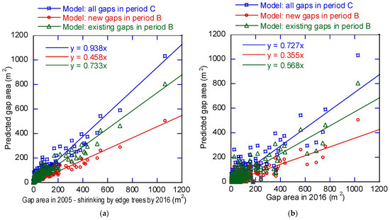
Figure 10.
Gap area prediction. (a) Predicted gap area after shrinkage by lateral growth of edge trees; (b) predicted gap area after shrinkage by lateral growth of edge trees and understory vegetation growth, and expansion.
From model (10) for 11 years of period C, we obtained a model predicting the duration N (years) until gap closure (gap lifespan).
N = (ln (5) – ln(A0)) × 11/ln (0.595)
The gap duration in 2005 and 2016 predicted by this model (Figure 11) was based on the initial gap area, and larger gaps had a longer duration. By 2016, many of the gaps present in 2005 were smaller, caused by shrinking, splitting, and closing; predicted lifespan was also greatly reduced. However, a new gap appeared in 2016 (lower center, Figure 11b).
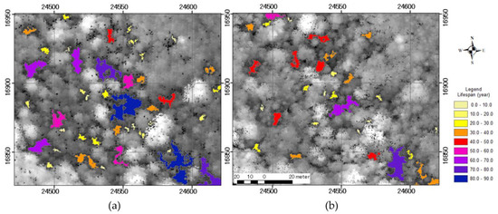
Figure 11.
Gap lifespan predicted by the relationship between initial gap area and shrinkage. (a) Prediction using the gap map in 2005 (b) and in 2016.
4. Discussion
4.1. Generating DCHMs and Extracting Gaps from LiDAR Data
The DSM pulse density influences the accuracy of gap extraction from LiDAR data [18]. For this reason, we examined the effects of pulse density differences between the three LiDAR datasets (Table 1) on gap extraction. In addition, deviations in pulse density within each DSM could affect gap extraction. The number of canopy openings < 5 m2 extracted differed significantly among the three DSMs; however, the number of gaps ≥ 5 m2 (a gap by our definition) was similar (Table 2). This indicates that differences in pulse density and deviation affected detection of small openings but not gaps. Thus, even though pulse density differed among the three DSMs, it had little effect on gap extraction.
4.2. Validation of Compatibility of Generated DSMs
Seasonal changes in foliage in deciduous forest can reduce the accuracy of gap extraction, and may have affected the LiDAR-2016 dataset obtained in October. Comparison of DSM-2016 and DSM-UAV images showed similar gap and canopy shapes (Figure 4). Although many smaller canopy openings were present in DSM-UAV (obtained in summer, 2018), those were not observed in DSM-2016. We confirmed that leaf-fall did not seriously affect gap extraction from LiDAR-2016.
Comparison of gap detection under different pulse densities using the simulated DSMs showed that 88.4% of the gap area in the simulated DSM based on LiDAR-2005 overlapped with the gap area in DSM-2016. Although lack of perfect gap overlap may have caused small errors in the detailed comparison of gaps, we confirmed trends in gap dynamics could be analyzed accurately by comparing the three LiDAR-DSMs.
4.3. Time-Series Tracking of Gap Generation and Canopy Closure
About 1000 gaps between 5.0 m2 and 1724.4 m2 were extracted from the three LiDAR-DSMs (Table 3). Reconstruction of gaps using the gap mask layer allowed us to summarize gaps that split or merged during the periods of the three LiDAR observations (Figure 3). Summarizing the gaps using the gap mask layer was an effective method to verify the spatial relationships of interacting gaps and their changes over the years. Mask layer processing showed that 15%, 28%, and 20% of the gaps present in 2005, 2011, and 2016, respectively, either merged or split (Table 3). Gaps with complicated shapes had a higher chance of interacting with surrounding gaps. This suggests that gaps tend to change shape by interaction with other gaps rather than alone. Summarizing the interacting gaps using the gap mask layer showed that the maximum gap area enlarged by between 1.6 and 1.9 times (Table 3), indicating that gap interaction had a marked impact on gap dynamics.
The greatest change occurred in 2011 among the 3 years (Table 3) and the reasons are as follows. There was no big disturbance in the period A and gaps tended to shrink and split into some parts. They were counted as one gap in 2011 after the mask layer operation. Above all, a big snowfall caused a disturbance in 2014 [45], and gaps expanded and merged with each other in the period B. Quite a few adjacent gaps in 2011 merged in the period B. These gaps were also counted as one gap by the mask operation. These situations probably caused high decrease of gap number in 2011 by the mask layer operation.
The ratio of gaps in different size classes was almost identical across the three periods (Figure 5); however, the number and ratio of new gaps and closing gaps differed between the two periods (Figure 6 and Figure 7). Similar trends were reported in an old growth mixed forest in the subarctic zone [26]. More new gaps appeared in period B than in period A (Table 4).
On the other hand, more gaps closed in period A than in period B. Changes in total gap number and total gap area differed between the periods. Total gap area decreased in period A by closure (Figure 5 and Figure 7, Table 4), but formation and expansion of gaps far exceeded closure in period B (Figure 6, Table 4). These results suggest that a fairly large disturbance occurred in the forest in period B. A typhoon caused damage in October 2004 [44], as did snow in December 2014 [45], and these events were probably the major causes of the changes in gap number, which was greatest in 2005, decreased in 2011, and increased in 2016. In a study conducted in a subarctic mixed forest, strong disturbance significantly impacted the number of gaps <15 m2, which were frequently formed by falling trees or branches, and number of small gaps changed similarly to our result [26]. For gaps <15 m2, the cycle from opening to closing is short because of their small size. Gap closure is prevented and many new gaps emerge if a disturbance occurs. Therefore, the number of gaps <15 m2 increases rapidly as a result. However, gap expansion occurred more frequently here than gap formation (Table 4), and this was also observed in the subarctic mixed forest [26].
Gaps with longer duration tended to expand via disturbances, perhaps because they experienced a greater number of disturbances (Table 4). Gap interaction via disturbance appears to be an important factor that increases gap lifespan, since interactions that increased gap area between 1.6 and 1.9 times occurred in large gaps. Longer gap lifespan also increases the chance of regeneration of understory vegetation. Mapping interacting gaps will show gap regeneration potential.
4.4. Modeling of Gap Reduction and Predicting Gap Lifespan
Gap closure was strongly dependent on initial gap area (Figure 8). During the six years of period A, gaps <15 m2 decreased to about one-fourth their original number, and decreased to about one-ninth their original number during the 11 years of period C. Small gaps that close by lateral growth of surrounding trees over a short period do not result in regeneration, although understory vegetation is present. On the other hand, all of the gaps ≥60 m2 were still present after 11 years. The light conditions needed for regeneration of undergrowth are removed when gaps close [50]. Therefore, understanding the factors underlying shrinkage and closure of gaps is important to understand the conditions required for regeneration.
Analysis of the relationship between initial gap area and shrinkage showed that shrinkage was proportional to the initial gap area, at least over the 11 years of the study period (Figure 9). Gap area decreased faster in new gaps than in existing gaps based on regression analysis of interpreted and predicted gap area (Figure 10a). This suggests that trees quickly extend branches horizontally when adjacent openings appear and that expansion speed decreases with time.
Among the three models, the gap reduction model (10) for period C predicted the slowest closure (Figure 10a). Model (10) was created by using new and existing gaps for periods A and B for a longer period than period A and B. Model (10) predicted gap reduction more accurately than models (11) and (12), which were based on shorter periods. Since tree crown size has a limit, reduction speed by canopy expansion is expected to decrease with time. When factors (a), (b), and (c) (Figure 10b) were included, the regression slope in the model verification was ~0.77 times the slope when only factor (a) was considered (Figure 10a). This means that the main factor in gap reduction was the lateral growth of gap edge trees (a), but that understory vegetation growth (b) and gap expansion (c) also affected gap dynamics considerably.
We mapped predicted gap lifespan using the gap maps for 2005 and 2016 and Equation (13) which was created based on Equation (10) (Figure 11). When we compared the prediction maps, some gaps with a long predicted lifespan based on the 2005 maps shrunk markedly and the predicted lifespan was reduced by more than 20 years. The average and the upper limit of understory vegetation growth were 0.15 m and 0.33 m year−1, respectively. Based on annual growth, seedlings were expected to grow > 5 m after 34 years on average and after 16 years at the earliest. Seedlings on the forest floor in gaps can regenerate, if gaps are large and last long enough. On the 2005 map, there are some gaps with a predicted lifespan > 40 years (Figure 11a), in which we expect regeneration to occur. However, predicted gap area and gap lifespan differed markedly in 2016, offering less potential for regeneration (Figure 11b).
Gap maps that show gap distribution, size, and lifespan will provide reference information for monitoring gap dynamics. Newer gaps showed faster shrinkage because of rapid growth of trees at the gap edges in the deciduous broadleaf forest. This meant that certain conditions, such as sufficient gap area and gap expansion by disturbance, were required for the regeneration of understory seedlings. Summarizing gaps by area classes can clarify the gap dynamics of a forest community. Precise evaluation of the effects of lateral growth at each height layer and of increases in the height of understory vegetation by location will be important for future long-term monitoring.
5. Conclusions
Gaps play an important role in forest regeneration, since gap formation prompts growth of seedlings on the forest floor. Gap dynamics are one of the key factors that influence forest structure and biodiversity, and provide important knowledge for forest management. Interactions between gaps, such as merging and splitting, make monitoring complicated, and we developed a procedure to summarize gaps stably by using LiDAR data from 2005, 2011, and 2016 and constructing a gap mask layer. The gap mask layer consistently described gap dynamics such as emergence, expansion, shrinkage, and merging of gaps. We showed a strong correlation between initial gap area and gap shrinkage. New gaps shrunk faster than existing gaps, and the rate of gap closure decreased with time according to regression analysis results. This result suggests that trees can rapidly extend branches into an adjacent open space following a disturbance, but that trees cannot constantly expand their canopies over a long period, because of limits on expansion distance. Comparison of predictions of gap lifespan based on 2005 and 2016 gap maps showed clear changes in gap area and predicted gap lifespan. We confirmed that large gap area, interactions among adjacent gaps, and expansion by disturbance are the requirements for longer gap duration for regeneration of understory vegetation. Here, we clarified the gap dynamics in a rather young (<100 years) deciduous broadleaf forest. An important next step will be predicting disturbance, to better predict the state of forest gaps. Validating spatiotemporal changes in various forest types under different successional stages will also be important to understand gap dynamics.
Author Contributions
Conceptualization and methodology, K.A. and Y.A.; resources and software, Y.A.; formal analysis, K.A.; field survey, K.A. and Y.A.; data curation, K.A.; visualization, K.A. and Y.A.; writing—original draft preparation, K.A.; writing—review and editing, Y.A.; supervision, Y.A.; research administration and funding acquisition, Y.A. All authors have read and agreed to the published version of the manuscript.
Funding
This research was executed in the undergraduate course program by Gifu University’s fund.
Institutional Review Board Statement
Not applicable.
Informed Consent Statement
Not applicable.
Data Availability Statement
The data presented in this study are available on request from the corresponding author after concluding a joint research agreement with River Basin Research Center of Gifu University. Restrictions apply to the availability of LiDAR2016, Ortho2003 and Ortho2016. These data were obtained from the Gifu Prefecture Government and are available by applying for the usage of them to the Gifu Prefecture Government.
Acknowledgments
We express heartfelt gratitude to Yasuyuki Maruya, a former Research Associate of the River Basin Research Center (currently an Assistant Professor at Kyushu University), Fuku Uekanekuri (Faculty of Applied Biological Sciences at that time), and Tomoko Onodera (Graduate School of Natural Science and Technology at that time) at Gifu University. We also express our gratitude to Kouji Suzuki and Hajime Hiratsuka, staff members of Takayama Research Center, River Basin Research Center. We appreciate the helpful comments and suggestions on the manuscript provided by Associate Professor Akemi Itaya at Mie University. The authors also wish to acknowledge the two anonymous reviewers for their helpful comments. The 2016 LiDAR data and the 2003 and 2016 aerial photographs were provided by Gifu Prefecture Government. We also express our gratitude to the government and its staff who supported our study.
Conflicts of Interest
The authors declare no conflict of interest.
References
- Nakashizuka, T.; Iida, S. Composition, dynamics and disturbance regime of temperate deciduous forests in Monsoon Asia. Vegetatio 1995, 121, 23–30. [Google Scholar] [CrossRef]
- Yamamoto, S. Forest Gap Dynamics and Tree Regeneration. J. Res. 2000, 5, 223–229. [Google Scholar] [CrossRef]
- Marks, P.L. The role of pin cherry (Prunus pensylvancia l.) in the maintenance of stability in northern hardwood ecosystems. Ecol. Monogr. 1974, 44, 73–88. [Google Scholar] [CrossRef]
- Yamamoto, S. Gap characteristics and gap regeneration in subalpine old-growth coniferous forests, central Japan. Ecol. Res. 1995, 10, 31–39. [Google Scholar] [CrossRef]
- Ishizuka, M.; Ochiai, Y.; Utsugi, G. Micro-environment and growth in gaps. In Diversity and Interaction in a Temperate Forest Community: Ogawa Forest Reserve of Japan; Nakashizuka, T., Matumoto, Y., Eds.; Ecological Studies; Springer: Tokyo, Japan, 2002; Volume 158, pp. 229–244. [Google Scholar]
- Sumita, A. Spatial structure of hardwood forest communities-individual based approaches. Jpn. J. Ecol. 1996, 46, 31–44, (In Japanese with English Summary). [Google Scholar]
- Ishida, M. Height distribution types and regeneration traits of main tree species in Quercus serrata-Pinus densiflora secondary forest. J. Jpn. For. Soc. 1996, 78, 410–418, (In Japanese with English Summary). [Google Scholar]
- Yamamoto, S.; Nishimura, N. Canopy gap formation and replacement pattern of major tree species among developmental stages of beech (Fagus crenata) stands, Japan. Plant Ecol. 1999, 140, 167–176. [Google Scholar] [CrossRef]
- Gendreau-Berthiaume, B.; Kneeshaw, D. Influence of Gap Size and Position within Gaps on Light Levels. Int. J. For. Res. 2009. [Google Scholar] [CrossRef]
- Miura, M.; Manabe, T.; Nishimura, N.; Yamamoto, S. Forest canopy and community dynamics in a temperate old-growth evergreen broad-leaved forest, south-western Japan: A 7-year study of a 4-ha plot. J. Ecol. 2001, 89, 841–849. [Google Scholar] [CrossRef]
- Tanouchi, H.; Yamamoto, S. Structure and regeneration of canopy species in an old-growth evergreen broad-leaved forest in Aya district, southwestern Japan. Vegetatio 1995, 117, 51–60. [Google Scholar] [CrossRef]
- Leeuwen, M.; Nieuwenhuis, M. Retrieval of forest structural parameters using LiDAR remote sensing. Eur. J. For. Res. 2010, 129, 749–770. [Google Scholar] [CrossRef]
- Wulder, M.A.; White, J.C.; Nelson, R.F.; Næsset, E.; Ole Ørka, H.; Coops, N.C.; Hilker, T.; Bater, C.W.; Gobakken, T. Lidar sampling for large-area forest characterization: A review. Remote Sens. Environ. 2012, 121, 196–209. [Google Scholar] [CrossRef]
- Tanaka, H.; Nakashizuka, T. Fifteen years of canopy dynamics analyzed by aerial photographs in a temperate deciduous forest, Japan. Ecology 1997, 78, 612–620. [Google Scholar] [CrossRef]
- Fujita, T.; Itaya, A.; Miura, M.; Manabe, T.; Yamamoto, S. Long-term canopy dynamics analyzed by aerial photographs in a temperate old-growth evergreen broad-leaved forest. J. Ecol. 2003, 91, 686–693. [Google Scholar] [CrossRef]
- Taguchi, H.; Furukawa, K.; Endo, T.; Sawada, H.; Yasuoka, Y. Monitoring of forest canopy using digital canopy models generated by multi-temporal aerial photographs. J. Jpn. Soc. Photogramm. Remote Sens. 2009, 48, 4–14, (In Japanese with English Summary). [Google Scholar]
- Torimaru, T.; Itaya, A.; Yamamoto, S. Quantification of repeated gap formation events and their spatial patterns in three types of old-growth forests: Analysis of long-term canopy dynamics using aerial photographs and digital surface models. For. Ecol. Manag. 2012, 284, 1–11. [Google Scholar] [CrossRef]
- Vepakomma, U.; St-Onge, B.; Kneeshaw, D. Spatially explicit characterization of boreal forest gap dynamics using multi-temporal lidar data. Remote Sens. Environ. 2008, 112, 2326–2340. [Google Scholar] [CrossRef]
- Kato, A.; Ishii, H.; Enoki, T.; Kobayashi, T.; Umeki, K.; Sakai, T.; Matsue, K. Application of laser remote sensing to forest ecological research. J. Jpn. For. Soc. 2014, 96, 168–181, (In Japanese with English Summary). [Google Scholar] [CrossRef]
- Lefsky, M.A.; Cohen, W.B. Selection of Remotely Sensed Data. In Remote Sensing of Forest Environments: Concepts and Case Studies; Wulder, M.A., Franklin, S.E., Eds.; Kluwer Academic Publishers: Norwell, MA, USA, 2003; pp. 13–46. [Google Scholar]
- Awaya, Y.; Tanaka, N.; Tanaka, K.; Takao, G.; Kodani, E.; Tsuyuki, S. Stand parameter estimation of artificial evergreen conifer forests using airborne images: An evaluation of seasonal difference on accuracy and best wavelength. J. For. Res. 2000, 5, 247–258. [Google Scholar] [CrossRef]
- Franklin, S.E.; Hall, R.J.; Smith, L.; Gerylo, G.R. Discrimination of conifer height, age and crown closure classes using Landsat-5 TM imagery in the Canadian Northwest Territories. Int. J. Remote Sens. 2003, 24, 1823–1834. [Google Scholar] [CrossRef]
- Awaya, Y.; Takahashi, T.; Kiyono, Y.; Saito, H.; Shimada, M.; Sato, T.; Toriyama, J.; Monda, Y.I.; Nengah, S.J.M.; Buce, S.; et al. Monitoring of peat swamp forest using PALSAR data-A trial of double bounce correction. J. For. Plann. 2014, 18, 117–126. [Google Scholar]
- Soja, M.; Persson, H.; Ulander, L. Estimation of forest height and canopy density from a single InSAR correlation coefficient. IEEE Geosci. Remote Sens. Lett. 2015, 12, 646–650. [Google Scholar] [CrossRef]
- Beraldin, J.; Blais, F.; Lohr, U. Laser Scanning Technology. In Airborne and Terrestrial Laser Scanning; Vosselman, G., Mass, H., Eds.; Whittles Publishing: Scotland, UK, 2010; pp. 19–30. [Google Scholar]
- Vepakomma, U.; Kneeshaw, D.; Fortin, M.J. Spatial contiguity and continuity of canopy gaps in mixed wood boreal forests: Persistence, expansion, shrinkage and displacement. J. Ecol. 2012, 100, 1257–1268. [Google Scholar] [CrossRef]
- Vepakomma, U.; St-Onge, B.; Kneeshaw, D. Response of a boreal forest to canopy opening: Assessing vertical and lateral tree growth with multi-temporal lidar data. Ecol. Appl. 2011, 21, 99–121. [Google Scholar] [CrossRef]
- Vepakomma, U.; Kneeshaw, D.; St-Onge, B. Interactions of multiple disturbances in shaping boreal forest dynamics: A spatially explicit analysis using multi-temporal lidar data and high-resolution imagery. J. Ecol. 2010, 98, 526–539. [Google Scholar] [CrossRef]
- Schreier, H.; Lougheed, J.; Tucker, C.; Leckie, D. Automated measurements of terrain reflection and height variations using an airborne infrared laser system. Int. J. Remote Sens. 1985, 6, 101–113. [Google Scholar] [CrossRef]
- Hirata, Y. Relationship between Tree Height and Topography in a Chamaecyparis obtusa Stand Derived from Airborne Laser Scanner Data. J. Jpn. For. Soc. 2005, 87, 497–503, (In Japanese with English Summary). [Google Scholar] [CrossRef][Green Version]
- Nelson, R.; Krabill, W.; Tonelli, J. Estimating forest biomass and volume using airborne laser data. Remote Sens. Environ. 1988, 24, 247–267. [Google Scholar] [CrossRef]
- Næsset, E. Estimating timber volume of forest stands using airborne laser scanner data. Remote Sens. Environ. 1997, 61, 246–253. [Google Scholar] [CrossRef]
- Lefsky, M.A.; Harding, D.; Cohen, W.B.; Parker, G.; Shugart, H.H. Surface lidar remote sensing of basal area and biomass in deciduous forests of eastern Maryland, USA. Remote Sens. Environ. 1999, 67, 83–98. [Google Scholar] [CrossRef]
- Maltamo, M.; Eerikäinenn, K.; Pitkänen, J.; Hyyppä, J.; Vehmas, M. Estimation of timber volume and stem density based on scanning laser altimetry and expected tree size distribution functions. Remote Sens. Environ. 2004, 90, 319–330. [Google Scholar] [CrossRef]
- Itoh, T.; Matsue, K.; Naito, K. Estimating forest resources using airborne LiDAR-Application of model for estimating the stem volume of Sugi (Cryptomeria japonica D. Don) and Hinoki (Chamaecyparis obtusa Endl.) by the tree height and the parameter of crown. J. Jpn. Soc. Photogramm. 2008, 47, 26–35, (In Japanese with English Summary). [Google Scholar]
- Takahashi, T.; Awaya, Y.; Hirata, Y.; Furuya, N.; Sakai, T.; Sakai, A. Stand volume estimation by combining low laser-sampling density LiDAR data with QuickBird panchromatic imagery in closed-canopy Japanese cedar (Cryptomeria japonica) plantations. Int. J. Remote Sens. 2010, 31, 1281–1301. [Google Scholar] [CrossRef]
- Awaya, Y.; Takahashi, T. Evaluating the differences in modeling biophysical attributes between deciduous broadleaved and evergreen conifer forests using low-density small-footprint LiDAR data. Remote Sens. 2017, 9, 572. [Google Scholar] [CrossRef]
- Ko, C.; Sohn, G.; Remmel, T.K.; Miller, J. Hybrid Ensemble Classification of Tree Genera Using Airborne LiDAR Data. Remote Sens. 2014, 6, 11225–11243. [Google Scholar] [CrossRef]
- Hovi, A.; Korhonen, L.; Vauhkonen, J.; Korpela, I. LiDAR waveform features for tree species classification and their sensitivity to tree- and acquisition related parameters. Remote Sens. Environ. 2016, 173, 224–237. [Google Scholar] [CrossRef]
- Awaya, Y.; Kameta, C.; Gotoh, S.; Miyasaka, S.; Unome, S. Classification of Sugi and Hinoki using high density airborne LiDAR data and two canopy shape parameters. Jpn. J. For. Plann. 2017, 51, 9–18, (In Japanese with English Summary). [Google Scholar]
- Nakatake, S.; Yamamoto, K.; Yoshida, N.; Yamaguchi, A.; Unome, S. Development of a single tree classification method using airborne LiDAR. J. Jpn. For. Soc. 2018, 100, 149–157, (In Japanese with English Summary). [Google Scholar] [CrossRef]
- Zhang, K. Identification of gaps in mangrove forests with airborne LIDAR. Remote Sens. Environ. 2008, 112, 2309–2325. [Google Scholar] [CrossRef]
- Choi, H.; Song, Y.; Jang, Y. Urban Forest Growth and Gap Dynamics Detected by Yearly Repeated Airborne Light Detection and Ranging (LiDAR): A Case Study of Cheonan, South Korea. Remote Sens. 2019, 11, 1551. [Google Scholar] [CrossRef]
- Gifu Prefecture Government Typhoon No 23 in 2004. Available online: https://www.pref.gifu.lg.jp/kurashi/bosai/shizen-saigai/11115/siryou/H16-taifuu23.html (accessed on 12 July 2020). (In Japanese).
- Snow and Ice Research Center (NIED) Snow Damage Survey in Hida area, Gifu Prefecture in December 2014–Flash News. Available online: https://www.bosai.go.jp/seppyo/kenkyu_naiyou/seppyousaigai/2015/quick%20report20150114gifu.pdf (accessed on 12 July 2020). (In Japanese).
- Fukuda, N.; Awaya, Y.; Kojima, T. Classification of forest vegetation types using LiDAR data and Quickbird images-Case study of the Daihachiga River Basin in Takayama city. J. JASS 2010, 28, 115–122, (In Japanese with English Summary). [Google Scholar]
- Masaharu, H. Map Projections-Technique on Geospatial Information; Asakura Publishing Co. Ltd.: Tokyo, Japan, 2011; pp. 19–26. (In Japanese) [Google Scholar]
- Campbell, J.B.; Wynne, R.H. Introduction to Remote Sensing, 5th ed.; The Guilford Press: New York, NY, USA, 2011; pp. 321–324. [Google Scholar]
- Watson, D.F.; Philip, G.M. A refinement of inverse distance weighted interpolation. Geo-Processing 1985, 2, 315–327. [Google Scholar]
- Abe, S.; Masaki, T.; Nakashizuka, T. Factors influencing sapling composition in canopy gaps of a temperate deciduous forest. Vegetatio 1995, 120, 21–32. [Google Scholar]


Publisher’s Note: MDPI stays neutral with regard to jurisdictional claims in published maps and institutional affiliations. |
© 2020 by the authors. Licensee MDPI, Basel, Switzerland. This article is an open access article distributed under the terms and conditions of the Creative Commons Attribution (CC BY) license (http://creativecommons.org/licenses/by/4.0/).