A Semi-Analytical Optical Remote Sensing Model to Estimate Suspended Sediment and Dissolved Organic Carbon in Tropical Coastal Waters Influenced by Peatland-Draining River Discharges off Sarawak, Borneo

Abstract

Coastal water quality degradation is a global challenge. Marine pollution due to suspended sediments and dissolved matter impacts water colour, biogeochemistry, benthic habitats and eventually human populations that depend on marine resources. In Sarawak (Malaysian Borneo), peatland-draining river discharges containing suspended sediments and dissolved organic carbon influence coastal water quality at multiple locations along the coast. Optical remote sensing is an effective tool to monitor coastal waters over large areas and across remote geographic locations. However, the lack of regional optical measurements and inversion models limits the use of remote sensing observations for water quality monitoring in Sarawak. To overcome this limitation, we have (1) compiled a regional spectral optical library for Sarawak coastal waters, (2) developed a new semi-analytical remote sensing model to estimate suspended sediment and dissolved organic carbon in coastal waters, and (3) demonstrated the application of our remote sensing inversion model on satellite data over Sarawak. Bio-optical data analysis revealed that there is a clear spatial variability in the inherent optical properties of particulate and dissolved matter in Sarawak. Our optical inversion model coupled with the Sarawak spectral optical library performed well in retrieving suspended sediment (bias = 3% and MAE = 5%) and dissolved organic carbon (bias = 3% and MAE = 8%) concentrations. Demonstration products using MODIS Aqua data clearly showed the influence of large rivers such as the Rajang and Lupar in discharging suspended sediments and dissolved organic carbon into coastal waters. The bio-optical parameterisation, optical model, and remote sensing inversion approach detailed here can now help improve monitoring and management of coastal water quality in Sarawak.

1. Introduction

Knowledge of the distribution of total suspended solids (TSS) and dissolved organic carbon (DOC) is essential for our understanding of water quality degradation and carbon cycle dynamics in coastal oceans. Coastal water quality degradation is a global challenge [1,2,3], which has particularly severe impacts on benthic habitats such as coral reefs [4,5] and seagrass meadows [6,7], and can change the structure, composition and extent of such ecosystems [8,9,10]. This can have knock-on effects on fish populations [11,12], for example by reducing species diversity and even causing species extinctions [13]. Increased DOC concentrations additionally affect ecosystem functioning by influencing water pH, transportation and reactivity of toxic substances, light absorbance, photochemistry and energy supply [14,15]. Thus, it is crucial to monitor TSS and DOC in coastal waters to improve our understanding of coastal water quality dynamics and to develop sustainable management strategies for coastal ecosystems.

Both TSS and DOC (the latter due to light absorption by coloured dissolved organic matter, CDOM) attenuate light and alter the spectral quality and quantity of light available for photosynthetic organisms. TSS plays a dual role in the aquatic ecosystem: it is an integral part of the food web and of nutrient cycles in natural waters [16,17], but it is also a pollutant in aquatic ecosystems. Among the many impacts on coastal and marine ecosystems [18], higher concentrations of TSS can lead to reduced fish egg survival [19], increased metabolic demand of coral reef sponges [20], reduced prey availability for marine mammals [21], decreased seagrass survival [22] and increased stress on coral reefs [23]. Thus, monitoring and management of TSS hotspots will help mitigate water quality impacts on coastal ecosystems.

Dissolved organic carbon in the oceans represents one of the largest pools of organic matter on Earth [24]. Coastal oceans play an essential role in the global carbon cycle as they form an interface between land and the deep ocean. Despite only covering ~4% of the global ocean surface, coastal oceans account for 14–30% of ocean primary production and 80% of organic matter burial [25]. Both autochthonous and allochthonous sources contribute DOC to the oceans. In coastal oceans, allochthonous DOC contributions are relatively high (~60% of total carbon) [26], but also highly variable due to climatic and anthropogenic drivers [27]. Upon reaching the coastal ocean, DOC impacts biogeochemical process and ecosystem functioning [14,28,29]. Thus, monitoring DOC transportation and transformation in coastal oceans is vital to improve our understanding of the global carbon cycle.

Traditional methods of measuring TSS and DOC require in-situ water sampling and laboratory analysis, which is expensive, laborious, time-consuming and weather-dependent. Recent advances in sensor technology have made it possible to monitor TSS and DOC at high temporal resolution with in-situ optical sensors [30,31,32]. However, each sensor can only provide data from a single geographical location, and so it remains a challenge to improve understanding of the larger-scale connections between source, pathway and sink. Another limitation of in-situ sensors is that each water quality parameter must be measured with a dedicated sensor, for example, optical scattering sensors for turbidity and TSS [33], fluorometers for chlorophyll and CDOM [31,34], and beam attenuation and absorption sensors for optical properties of water constituents [35]. Alternatively, in-situ measurements of reflectance spectra, coupled with a suitable bio-optical model, can be used to retrieve the concentrations of multiple biogeochemical components [36,37]. However, this reflectance-based approach has similarly limited spatial coverage.

Satellite ocean colour remote sensing has advanced significantly in the past two decades and can now provide biogeochemical data at high temporal and spatial resolution from hydrodynamically complex and remote ecosystems [38,39]. Initially, empirical algorithms were used to transform satellite optical observations into water-quality and biogeochemical parameters (see Ref. [40] and references therein). However, more sophisticated approaches are necessary to decouple the optical signatures and derive multiple water quality parameters in optically complex coastal waters [41,42], and most of the commonly available global ocean colour models do not provide TSS or DOC concentrations [43,44,45].

Coastal waters in Sarawak, Malaysia, host ecologically and economically valuable marine habitats and fish populations [46,47]. Land adjacent to ocean in Sarawak is mostly forested and includes large areas of coastal, tropical peatlands [48]. Climate change and anthropogenic activity in Sarawak are known to impact land cover and the suspended material discharged into the coastal oceans [49,50]. Previous studies in Sarawak mainly used in-situ water sampling to measure TSS and DOC [50,51], which only provides spatially and temporally limited insights into the processes driving variability. Remote sensing could significantly improve the resolution of water quality observations in Sarawak. For instance, a recent study proposed an algorithm to estimate riverine DOC fluxes from rivers in Sarawak [52]. Still, this work focused only on the immediate areas surrounding river plumes and only used an empirical band-ratio algorithm; it also did not address TSS retrieval. Thus, to our knowledge, there are no remote sensing algorithms that could retrieve both TSS and DOC concentrations either from in-situ sensors or from satellite-based sensors across coastal waters of Sarawak. Here, we provide the first analysis of bio-optical properties in coastal waters of Sarawak. The objectives of this study are to:

(1)

understand the variability of optical signatures in coastal waters of Sarawak;

(2)

develop a remote sensing inversion model coupled with a regional spectral optical library to estimate TSS and DOC using in-situ optical measurements;

(3)

demonstrate the application of this inversion model using MODIS Aqua satellite data for Sarawak coastal waters.

The bio-optical analysis, optical parameterisation, inversion modelling approach and remote-sensing products developed in this study will help coastal monitoring and management programs in tropical coastal waters of Sarawak.

2. Materials and Methods

2.1. Study Area

The state of Sarawak is part of the Federation of Malaysia and lies on the island of Borneo between 0°50′N and 5°N latitude and 109°36′E and 115°40′E longitude (Figure 1). It covers an area of 124,450 km² and has a population of about 2.8 million (Department of Statistics, Malaysia, 2018). Sarawak experiences a tropical rainforest climate characterised by uniform temperature, high humidity and intense rainfall, and is influenced by two monsoon periods: the wetter north-east monsoon (November–March) and the relatively drier south-west monsoon (May–September). Climate change is impacting temperatures and the annual cycle of precipitation in Sarawak, and these changes in rainfall have significantly influenced river discharge in most of the river basins of Sarawak [53].

Land cover in Sarawak state is mainly forested area (~64%), of which peat swamp forest occupies 6.1% (Forest Department, Sarawak, 2015). Deforestation in Sarawak for timber production and agriculture development has increased soil erosion in Sarawak rivers [54]. Along the coast in Sarawak, mangrove forests cover 60% of the total coastline. The mangrove forests in Sarawak have suffered from human expansion (agriculture and aquaculture) and pollution through industrialisation and urbanisation [46]. The primary cause of water quality degradation in Sarawak rivers and coastal waters is due to the release of excessive particulate and dissolved substances as a result of changing land cover and land use practices [54,55]. River discharges in Sarawak are known to impact the coastal biogeochemical oceanography in the South China Sea [56].

2.2. Field Survey Details

Three fieldtrips were conducted during 2017 to measure bio-optical properties in coastal waters of Sarawak (Figure 1). The sampling strategy in all the field trips was to collect measurements that represent turbid riverine water, coastal mixing and clear ocean waters. The first field trip was conducted during 8–13 June 2017 (hereafter denoted as SJ). A total of 26 stations were occupied in the suspended sediment-rich waters off the Rajang and Lupar rivers, where coastal peatlands additionally supply terrestrial DOC. Discrete water samples for bio-optical measurements were taken at 20 stations and apparent optical properties were measured during daylight conditions at 10 stations that covered turbid river, coastal and clear ocean locations.

The second field survey was undertaken during 4–10 September 2017 (hereafter denoted as SS). Measurements from this trip represent the ecosystem conditions just before the beginning of the north-east monsoon. A total of 26 field stations in SS covered similar coastal regions of Sarawak as in SJ. Water samples for spectrophotometric analysis (to measure absorption due to particulate and dissolved matter) were collected at 15 stations, backscattering measurements were taken at 24 stations and radiometric measurements made at 19 stations (daytime stations). During both SJ and SS surveys, all the samples were filtered and preserved directly on board the boat.

The third field survey was undertaken during 13–16 September 2017 (hereafter denoted as SM). This field trip covered 23 stations in the western-most area of Sarawak, where suspended sediment concentrations are lower and the peatland-draining Samunsam river provides a discharge of DOC-rich blackwater. Water samples for spectrophotometric analysis were taken at 10 stations, backscattering profiles at 15 stations and radiometric measurements at 16 stations. All stations during SM were sampled from a small outboard-powered boat, and water samples were stored in dark insulated boxes and filtered back on land each afternoon.

2.3. Biogeophysical Measurements

Surface water at each station was collected using a clean plastic bucket. Seawater (50–1000 mL) was filtered through pre-rinsed and pre-weighed glass fibre filters (Whatman GF/F, 0.7 µm, 25 mm) to collect Total Suspended Solids. Filters were cleaned with MilliQ water to remove any salt and stored at −20 °C until analysis. Filters were then dried to a constant weight at 75° C and re-weighed on a microbalance (1 µg readability). The full protocol used to determine TSS is available in [57].

Water for dissolved organic carbon (DOC) analysis was collected in amber glass bottles, and then filtered through a Whatman Anodisc filter (0.2 µm pore size) that was pre-rinsed with 1 M HCl, Milli-Q water, and sample water. The final filtrate (30 mL) was stored in an amber vial, acidified with 0.1 mL of 50% H₂SO₄ and stored in a refrigerator at 4 °C. Once in the laboratory, DOC measurements were performed on a Shimadzu TOC-L system with a high-salt combustion kit. Instrument performance was monitored using certified deep-sea water from the Hansell Laboratory, University of Miami (42–45 µmol L⁻¹). Our analyses yielded a long-term value for the reference water of 47 ± 2.0 µmol L⁻¹ (mean ± 1 SD, n = 51). Procedural blanks prepared in the field almost all contained <10 µmol L⁻¹, except for those prepared in between blackwater river samples, which contained 13–27 µmol L⁻¹; a correction for these procedural blanks was not applied [58].

2.4. Optical Measurements

2.4.1. Inherent Optical Properties (IOP)

The spectral light absorption coefficient of natural waters (a_T) is the sum of light absorption due to optically active particulate and dissolved substances in the water:

a_T(λ) = a_W(λ) + a_P(λ) + a_Y(λ)

(1)

including contributions from water (a_W), particulate matter (a_P) and CDOM (a_Y). In some studies, particulate matter is further separated into contributions from phytoplankton and non-algal particulate matter [59,60]. In this study, the spectral range of λ = 400–700 nm is considered.

To collect CDOM, seawater was filtered as for DOC analysis, and 30-mL samples were preserved with 0.5 mL of a 10% w/v solution of sodium azide (NaN₃) solution and stored in amber vials at +4 °C until analysis. While this preservation method follows previous recommendations for remote sensing algorithm development [57], recent research cautions against using NaN₃ as a preservative for CDOM measurements due to blank effects in the ultraviolet range [61]. CDOM samples were analysed within a month of collection. They were brought to room temperature and their absorbance was measured from 230 to 900 nm against a DI water reference using a Thermo Evolution 300 dual-beam spectrophotometer. Instrument performance was checked according to [62]. Reagent blanks of NaN₃ in DI water showed no absorbance over the wavelength range considered here. CDOM spectra were baseline corrected [63] and converted to Napierian absorption coefficients following Equation (2):

a_Y(λ) = 2.303 × A_Y(λ)/l

(2)

where a(λ) and A(λ) are, respectively, the absorption coefficient and the absorbance at wavelength λ, and l is the cuvette pathlength in metres. The spectral slope of CDOM (S_Y) was determined by applying a non-linear exponential model to fit a_Y between 400 and 700 nm. Spectral CDOM absorption was then modelled as:

a_Y(λ) = a_Y(440) × exp(−S_Y × (λ − 440))

(3)

To measure aP, particles were filtered onto Whatman GF/F filters and stored flat in tissue embedding cassettes in liquid nitrogen until analysis (within three months). The optical density (OD) spectrum was measured over the 350–800 nm spectral range in 0.9 nm increments, using a Cintra 404 UV/VIS dual beam spectrophotometer equipped with an integrating sphere. The OD scans were converted to absorption spectra by first normalising the scans to zero at 750 nm and then correcting for the pathlength amplification using the coefficients of [62]. Unlike CDOM absorption, a_P does not have a functional form due to phytoplankton absorption peaks. Particulate absorption has contributions from both non-algal matter and phytoplankton. When dominated by non-algal matter, particulate absorption spectra show an exponential decrease [64], which could be modelled similar to CDOM absorption. However, with increasing phytoplankton presence, the total particulate absorption spectrum will deviate from this exponential behaviour and will include absorption peaks due to phytoplankton pigments (for example, at 443 and 676 nm). To represent such a complex behaviour, in this study spectral particulate absorption a_P(λ = 400–700 nm) was therefore modelled as a product of TSS concentration and the mass-specific particulate absorption spectra.

Specific inherent optical properties (SIOP) are computed by normalising IOP to their biogeochemical concentrations. This is useful in understanding and comparing the optical efficiency of particulate and dissolved substances [60]. In this study, mass-specific absorption values were computed for particulate (a_P*; m² TSS g⁻¹) and dissolved substances (a_Y* (m⁻¹ μM C⁻¹). Using these SIOP values for modelling purposes, total absorption could be rewritten as:

a_T(λ) = a_W(λ) + (TSS × a_P*(λ)) +(DOC × a_Y*(440) × exp(−S_Y × (λ−440)))

(4)

Total light backscattering in the water column can be expressed as:

b_bT(λ) = b_bW(λ) + b_bP(λ)

(5)

where b_bW is the backscattering due to seawater [65] and b_bP is the backscattering due to particulate matter suspended in the water column.

We measured light backscattering in the water column using a WET Labs ECO BB-9 instrument at wavelengths 412, 440, 488, 510, 532, 595,650, 676 and 715 nm. Raw data from the BB-9 is output as counts from the sensor. By applying the calibration procedure (subtracting the dark offset and multiplying by a scaling factor), the raw counts were converted to meaningful volume scattering coefficients, β_T(θ, λ) with units of m⁻¹ sr⁻¹. Measured β_T are further corrected for the absorption in the incident beam following the method suggested for the BB-9 using the spectrophotometric absorption values measured at each station (user guide, WET Labs ECO BB-9, 2017). The corrected volume scattering coefficients comprise contributions from particles and water in the backward direction (θ = 117°). Particulate volume scattering (β_P) was obtained by subtracting the volume scattering of water [65]. Particulate backscattering coefficients, b_bP(λ) with units of m⁻¹, were then determined as:

b_bP(λ) = 2 × π × X × β_P(117°)

(6)

For a diversity of water types, Boss and Pegau [66] suggested a value of 1.1 for the factor X, to convert scattering in an angle in the back direction to the backscattering coefficient (full details in WET Labs ECO BB-9, 2017).

The spectral slope of

b_bP(λ) = TSS × b_bP*(650) × (λ/650)^SbbP

(7)

In this study, total backscattering was then modelled as:

b_bT(λ) = b_bW(λ) + (TSS × b_bP*(650) × (λ/650)^SbbP)

(8)

Backscattering albedo (uT) is the ratio of total backscattering to the sum of total backscattering and total absorption [67,68]. Backscattering albedo directly influences the remote sensing reflectance and the light availability in the water column [69,70,71]. We computed the backscattering albedo using the BB-9 measured backscattering data and our spectrophotometric measurements of total absorption as:

uT(λ) = b_bT(λ))/(a_T(λ) + b_bT(λ))

(9)

2.4.2. Apparent Optical Property Measurements

In this study, hyperspectral (320–950 nm at 2 nm resolution) radiometric measurements were made using Trios-RAMSES radiometers (https://www.trios.de/en/ramses.html). Apparent optical properties (AOP) of the water column such as above-surface downwelling irradiance Es(0+, λ), underwater downwelling irradiance Ed(depth, λ) and upwelling radiance Lu(depth, λ) were measured. Deployment of instruments followed the protocols suggested in [72]; the radiance sensor had a field of view of 7°. Measurements were made only during high sun elevation conditions (10 AM to 4 PM during the day) under stable sun and sky conditions.

During the September fieldtrip, we could not deploy the radiometers in the profiling mode due to difficult weather and ocean conditions. In this trip, the radiometers were deployed using a surface float to measure Lu(0−, λ) and Ed(0+, λ), which were further used to compute the remote sensing reflectance Rrs(λ) following:

R_rs(λ,0+) = ((1 − ρ)/n²) × (Lu(0−,λ)/Ed(0+,λ))

(10)

where ρ (=0.021) is the Fresnel reflectance and n (1.34) is the refractive index of water [72]. Above-surface remote sensing reflectance R_rs(λ,0+) was converted to underwater (just below the surface) remote sensing reflectance r_rs(λ,0−) using the relationship below [67,73]:

r_rs(λ,0−) = R_rs(λ,0+)/(0.52 + 1.7 × R_rs(λ,0+))

(11)

Hyperspectral R_rs was then converted to MODIS band equivalent values by convolving with the MODIS AQUA spectral response function values (available at https://oceancolor.gsfc.nasa.gov/docs/rsr/rsr_tables/). A strong relationship between single and band R_rs was noted (R_rs(λ) = 0.5343 × R_rs(MODIS bands), R² = 0.99), which was used to generate R_rs at MODIS AQUA central wavelengths and supply it as an input to the inversion model.

2.4.3. Relationship between Underwater Remote Sensing Reflectance and Backscattering Albedo

Remote sensing reflectance just below the surface, r_rs(0−) is known to vary as a function of single scattering albedo, as described by the following equation [67,71]:

r_rs(0−) = (f/Q) × uT

(12)

where f indicates the relationship between irradiance reflectance and IOPs ([74] and references therein) and Q (ratio of upwelling radiance to irradiance) [75] represents the directional nature of upwelling light field. The term f/Q is equivalent to G0(uT) + G1(uT), and r_rs(0−) could be rewritten as below:

r_rs(0−) = (G0 × (uT) + G1 × (uT)) × uT

(13)

where G0 and G1 represent the combined influence of illumination, sea surface conditions and marine volume scattering function [73]. For a given r_rs(0−), uT could also be derived by rewriting the above equation as:

uT = (− G0 + [G0 + 4 × G1 × r_rs(0−)]^1/2)/(2 × G1)

(14)

Measurements of r_rs(0−) and uT from this study were used in the equations above to estimate regional G0 and G1 values for Sarawak coastal waters.

2.5. Statistics

We describe the variation in bio-optical properties using their minimum and maximum values, and their mean and percent coefficient of variance (% CV = 100 (standard deviation/mean)). Relationships between parameters were assessed using linear correlation (r). Strength of regression was described using the coefficient of determination (R²). The performance of optical models was evaluated using bias and mean absolute error (MAE), which were computed following Seegers et al. [76]. We used log-transformed data when computing bias and MAE, as the data span multiple orders of magnitude. For interpretation purposes, they were converted out of log10 space. Bias values closest to unity are considered least biased and values less than unity indicate a negative bias. MAE indicates the average magnitude of model errors, where the increase above unity indicates the relative measurement error (i.e., MAE = 1.00 means no error, while 1.10 means 10% error). Mean percent relative deviation (MPRD(%) = mean(100 (model − measurement)/measurement) was used to compare the simulated and measured optical signature (uT or R_rs).

2.6. Remote Sensing Data

Satellite remote sensing data from the MODIS Aqua sensor were used to demonstrate the application of the remote sensing inversion model. MODIS Aqua has bands at 412, 443, 488, 531, 555, 667, and 678 nm in the visible region. We downloaded Level-2 reflectance products from https://oceancolor.gsfc.nasa.gov/, which are atmospherically corrected [77] and are reported to have good performance in multiple water types [78]. However, in some pixels in coastal waters close to land, the atmospheric correction fails (resulting in negative remote sensing reflectance), which are flagged and removed before the inversion model is applied. For demonstration purposes, relatively cloud-free MODIS Aqua images were used.

3. Modelling Results and Discussion

3.1. Model Structure

The remote sensing inversion model developed in this study has three main components (Figure 2): (1) a regional spectral optical library of specific inherent optical properties, (2) a forward model to simulate total absorption, total backscattering and backscattering albedo, and (3) an inversion mechanism to derive biogeochemical parameters through spectral matching of remote sensing and forward-modelled backscattering albedo. The model is sufficiently flexible to be applied to both in-situ and satellite-measured remote-sensing reflectance. The model components are described in detail in Section 3.2, Section 3.3, Section 3.4, Section 3.5 and Section 3.6.

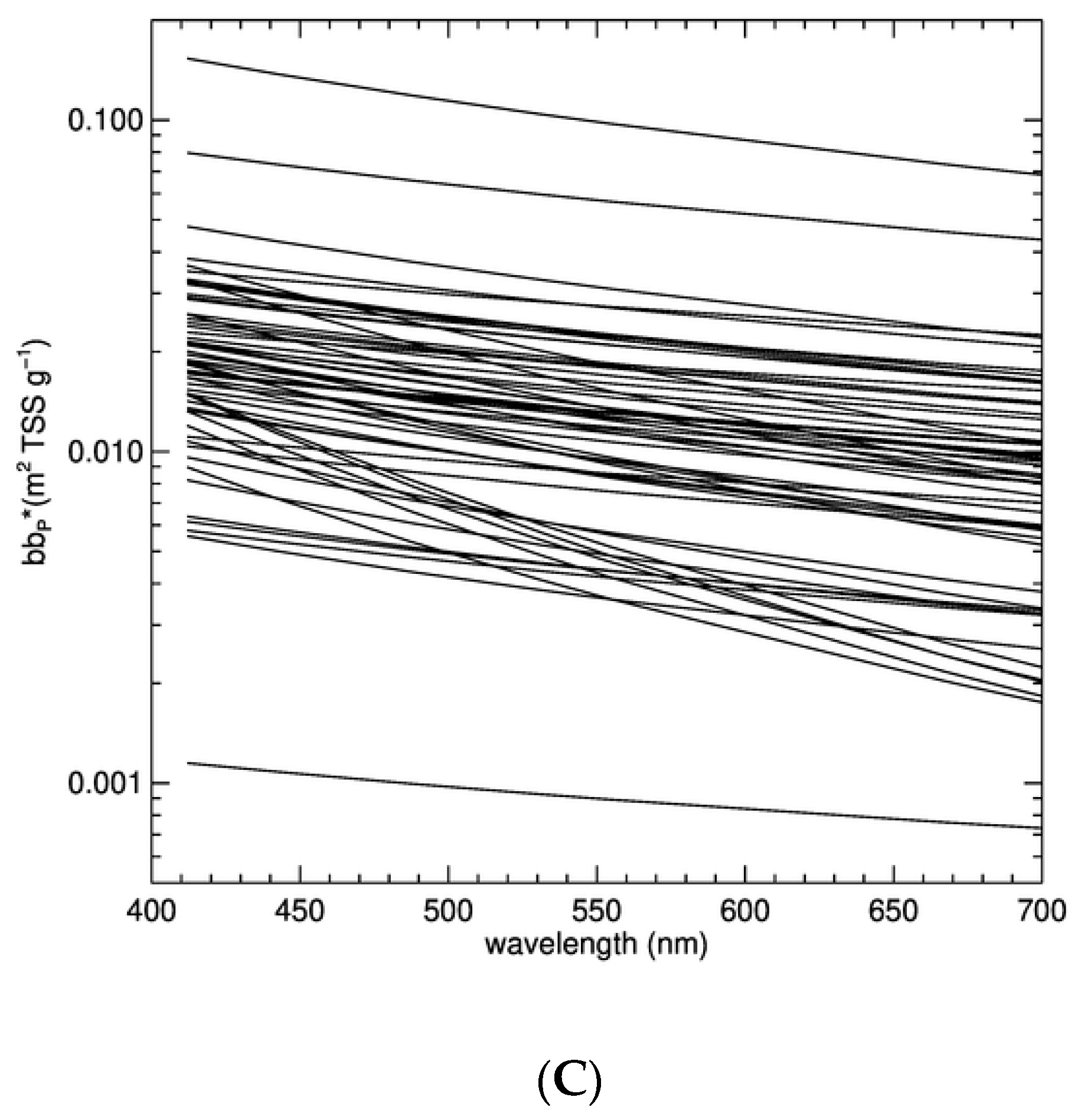
3.2. Regional Spectral Optical Library

We compiled a regional Sarawak spectral optical library (SSOL; Figure 3) for use in the optical model. The data used for this model was collected during June and September 2017, which represent coastal ecosystem conditions during different monsoon periods. SSOL mainly includes specific inherent optical properties that help simulate total absorption, total backscattering and backscattering albedo as described in Equations (4), (8) and (9).

Our measured a_P*(λ) varied over a wide range (Figure 3A), with higher values in the blue region and relatively lower values in the green-red region. Similar to coastal waters elsewhere [64,68,79,80,81], the spectral shape of a_P* varied due to the changing composition of particulate matter. In clear waters, with mainly phytoplankton as particulate matter, a_P* spectra clearly showed absorption peaks around 443 and 676 nm. In contrast, increasing concentrations of non-algal particulates masked the phytoplankton absorption peaks in more turbid coastal waters, yielding a_P* spectra that decrease towards the red region. Due to the presence of phytoplankton absorption peaks, the a_P*(λ) could not be written in a functional form; for this reason, the full-spectrum a_P* values were included in SSOL. The spectral library does not explicitly separate particulate absorption into phytoplankton and non-algal particulate matter, as our focus was on distinguishing between CDOM and particulate absorption. However, the spectral library could easily be expanded to include subgroups of particulate matter if necessary.

Sarawak coastal waters are overall rich in CDOM (

Table 1. Observed bio-optical variability in Sarawak coastal waters during 2017 field trips.

	SJ2017		SS2017		SM2017
Parameter [Units]	[N] Min.–Max.	Mean (CV%)	[N] Min.–Max.	Mean (CV%)	[N] Min.–Max.	Mean (CV%)
Temperature [°C]	[23] 28.8–31.6	30.0 (2.2)	[25] 26.6–30.9	28.8 (4.1)	[20] 28.6–31.5	30.33 (2.3)
Salinity	[23] 4.7–32.2	25.5 (31.8)	[19] 18.6–31.9	28.5 (13.9)	[20] 2.0–32.5	28.0 (28.2)
TSS, [mg L−1]	[24] 1.1–174.6	29.8 (134.8)	[21] 0.56–174.5	23.9 (164.8)	[20] 0.5–10.5	3.8 (86.5)
DOC, [µMC]	[25] 80.9–209.3	120.7 (31.4)	[22] 76.0–166.3	106.7 (26.8)	[21] 76.2–1798.7	330.0 (142.4)
aY(440) [m−1]	[25] 0.2219–2.834	1.1362 (77.7)	[24] 0.1009–1.858	0.627 (79.2)	[20] 0.0457–23.97	3.6102 (194.5)
aY*(440) [m−1 µMC−1]	[25] 0.0027–0.0203	0.0083 (57.7)	[19] 0.0013–0.0162	0.0047 (76.5)	[20] 0.0006–0.0148	0.0045 (112.6)
SY(x–1.) [nm−1]	[25] 0.0088–0.0182	0.0161 (11.4)	[24] 0.0047–0.021	0.0138 (29.5)	[20] 0.0138–0.0181	0.0159 (7.9)
bbP(650) [m−1]	[21] 0.0016–0.7057	0.2416 (103.3)	[23] 0.0015–2.48	0.2896 (191.3)	[15] 0.0112–0.168	0.0462 (94.0)
bbP*(650) [m2 TSS g−1]	[20] 0.0036–0.0246	0.0097 (50.9)	[19] 0.0008–0.0765	0.0014 (125.9)	[14] 0.0034–0.0239	0.0147 (41.39)
Sbbp(x–1.) [nm−1]	[21] 0.93–2.39	1.69 (28.7)	[23] 0.40–3.75	1.3 (55.1)	[15] 0.76–1.33	1.1 (13.6)
aP*(412) [m2 TSS g−1]	[16] 0.0567–0.4469	0.1684 (59.6)	[16] 0.0157–0.1596	0.1034 (45.5)	[11] 0.1029–0.6294	0.2301 (77.9)
aP*(443) [m2 TSS g−1]	[16] 0.0451–0.2213	0.1008 (48.8)	[16] 0.0157–0.121	0.0718 (39.25)	[11] 0.0708–0.4144	0.1607 (71.25)
aP*(488) [m2 TSS g−1]	[16] 0.0268–0.1138	0.0585 (44.9)	[16] 0.0091–0.0769	0.0441 (42.9)	[11] 0.04418–0.2529	0.0979 (73.7)
aP*(531) [m2 TSS g−1]	[16] 0.0136–0.0516	0.0284 (40.7)	[16] 0.0037–0.0337	0.0206 (41.4)	[11] 0.0230–0.1614	0.0556 (90.4)
aP*(555) [m2 TSS g−1]	[16] 0.0095–0.0315	0.0184 (37.1)	[16] 0.0026–0.0198	0.0134 (35.5)	[11] 0.0144–0.1249	0.0412 (97.8)
aP*(667) [m2 TSS g−1]	[16] 0.0026–0.0178	0.0060 (62.8)	[16] 0.0026–0.0187	0.0064 (63.4)	[11] 0.0063–0.0354	0.0183 (54.3)
aP*(678) [m2 TSS g−1]	[16] 0.00218–0.0204	0.0058 (76.7)	[16] 0.0021–0.0217	0.0067 (73.9)	[11] 0.0060–0.0301	0.0169 (52.3)

). The highest CDOM absorption was found in the Samunsam and Sematan river mouths in the western part of study area (measured during SM2017; Figure 1). In the coastal waters influenced by the Rajang River, mean values of a_Y(440) were similar in June and in September 2017. Our CDOM absorption values for Sarawak are similar to values reported from the Mahakam Delta (Indonesian Borneo) and surrounding coastal waters (mean a_Y(440) = 0.87 m⁻¹) [82], but on average higher than the values measured off the east coast of Peninsular Malaysia both during the NE monsoon (0.15 m⁻¹) and at other times (0.05 m⁻¹) [80]. The spectral slope of CDOM is a good indicator of the origin of CDOM, with higher values (about 0.021 nm⁻¹) associated with marine sources and lower values (about 0.014 nm⁻¹ associated with terrestrial sources) [83]. In addition to these two groups, in Sarawak coastal waters we also observed spectral values lower than 0.01 nm⁻¹ in 6% of the samples (occurring both in clear and turbid waters). Analysis of fluorescence spectra has shown that DOC and CDOM in the coastal waters of our study region was to a large degree terrestrial in origin, with peatlands representing the main terrestrial source [84]. The absorption efficiency (as indicated by a_Y*) of CDOM varied by two orders of magnitude in the western part of the study area, where both the blackwater Samunsam River and relatively clear marine waters were sampled (Table 1; SM2017). In the eastern part of the study area, a_Y* covered a similar range during both the June and September field trips, which was smaller than in the western region. Overall, this dataset indicates that the CDOM absorption properties vary most strongly spatially rather than temporally in coastal waters of Sarawak. This is consistent with previous analysis of the mixing behaviour of DOC and CDOM, which found that there was a single, strong relationship between DOC and CDOM in our dataset across all seasons [58]. Notably, Martin et al. [58] also included DOC and CDOM data for both the eastern and western area of our study region during March 2017, representing the end of the northeast monsoon (when other optical properties were not measured). The CDOM and DOC dataset used here was also used in [58] to analyse the biogeochemistry of dissolved organic matter in Sarawak, but that study reported other CDOM parameters than we use here (e.g., a_Y(350) and spectral slopes at UV wavelengths).

Light backscattering due to particulate matter also varied spatially more than temporally in Sarawak coastal waters (Table 1). Values of b_bP varied in response to changing TSS concentrations (linear correlation, r = 0.87) in coastal waters, with lower values in clear marine waters and higher values in turbid sediment-rich coastal waters near river mouths. Spatially, the mean b_bP(650) values were higher in the eastern region off the Rajang delta, and were slightly higher during September than June, although the range of values largely overlapped between the two seasons (Table 1). Regionally, b_bP values measured in Sarawak were comparable to those measured in the Mahakam delta [82], but were higher by an order of magnitude compared to values from the Berau estuary, Indonesian Borneo (b_bP(660) = 0.0345) [85], despite the relative proximity of the Mahakam and Berau rivers. The spectral shape of b_bP followed a hyperbolic function with spectral slopes (S_bbP) varying between 0.40 and 3.75 nm⁻¹, with mean values that are comparable to other coastal regions [59,85,86]. Higher values of S_bbP were found in the more TSS-rich eastern region than in the western region (Table 1). Higher values of S_bbP indicate smaller average particle diameters [86], and such small particles should offer larger surface area for photon interaction and increase the particulate backscattering efficiency. However, in this data set, we only observed a poor correlation (r = 0.25) between b_bP*(650) and S_bbP, suggesting that other particle characteristics (such as shape, composition and porosity; [87]) influenced the particulate backscattering efficiency. The backscattering efficiency covered a large and mostly overlapping range between the two regions and seasons, but was on average slightly higher in the western region (SM; Figure 1), and in June compared to September in the eastern region (Table 1). These results indicate that backscattering properties of particulate matter show especially spatial variability in Sarawak coastal waters, and bio-optical models for this region must therefore capture this variability.

The high spatial variability in the inherent optical properties of Sarawak reflects partly the diversity of river discharges: rivers originating in peatlands carry high CDOM and DOC concentrations but lower TSS concentrations, while rivers draining mineral soils carry high TSS but lower DOC and CDOM concentrations. It also reflects the strong on-shore to off-shore gradients in TSS and CDOM, as particles settle out beyond river plumes, and CDOM is diluted with water from the open sea and photobleached. These results highlight the limitation of extrapolating optical properties from one region to another. To incorporate this process- and region-specific variability, we categorised the spectral optical library into three optical water types (OWT): clear marine waters, turbid coastal waters, and highly turbid coastal waters (influenced by river discharges). Our classification of OWT was based on the reflectance signature: similar to Aurin et al. [71], we used the reflectance ratio to distinguish between highly turbid “red” waters (Type-3: R_rs(650):R_rs(443) > 1.5), coastal waters (Type-2: R_rs(650):R_rs(443) ≤ 1.5), and clear marine waters (Type-1: R_rs(650):R_rs(443) ≤ 0.05). Once categorised, each set of SIOPs (a_P*, a_Y* and b_bP*) is supplied to the optical model as a set and not as independent values, because they are associated together with an individual process (for example, a river plume). This treatment of sets of SIOPs helps to represent the optical properties in a realistic fashion, avoiding the random mixing of SIOPs that were never encountered in combination. Thus, each set of specific inherent optical properties was categorised and associated with one OWT. Such a categorisation helps the selection of realistic SIOP sets for inverse modelling.

3.3. Conversion of Underwater Remote Sensing Reflectance and Backscattering Albedo

Remote sensing reflectance just below the surface, r_rs(0−), varies as a function of single scattering albedo [67,71,88,89], and the coefficients G0 and G1 differ between clear ocean waters and turbid coastal waters (see Section 2.4.1). Fixed values of G0 = 0.0949 and G1 = 0.0794 were suggested for clear ocean waters by Gordon et al. [88] and G0 = 0.0895 and G1 = 0.1247 for coastal waters by Lee et al. [67]. In contrast, Aurin et al. [71] proposed a set of spectrally varying f/Q values for conversion (see Table 3 in [71]).

In Sarawak coastal waters, the parameterisations by Gordon et al. [88], Lee et al. [67], and Aurin et al. [71] generally underestimated uT values, even though they showed acceptable linearity, with the spectrally varying conversion factors of Aurin et al. [71], yielding slightly lower bias than the other two approaches (Figure 4A–C). To improve agreement between modelled and measured uT values, we used Sarawak region-specific values (G0 = 0.0508) and G1 = −0.0271), which were generated through optimisation of regional values of r_rs(0−) and uT. Using these Sarawak-specific values in the relationship between r_rs(0−) and uT (Equation (14)) resulted in a better match of uT (Figure 4D).

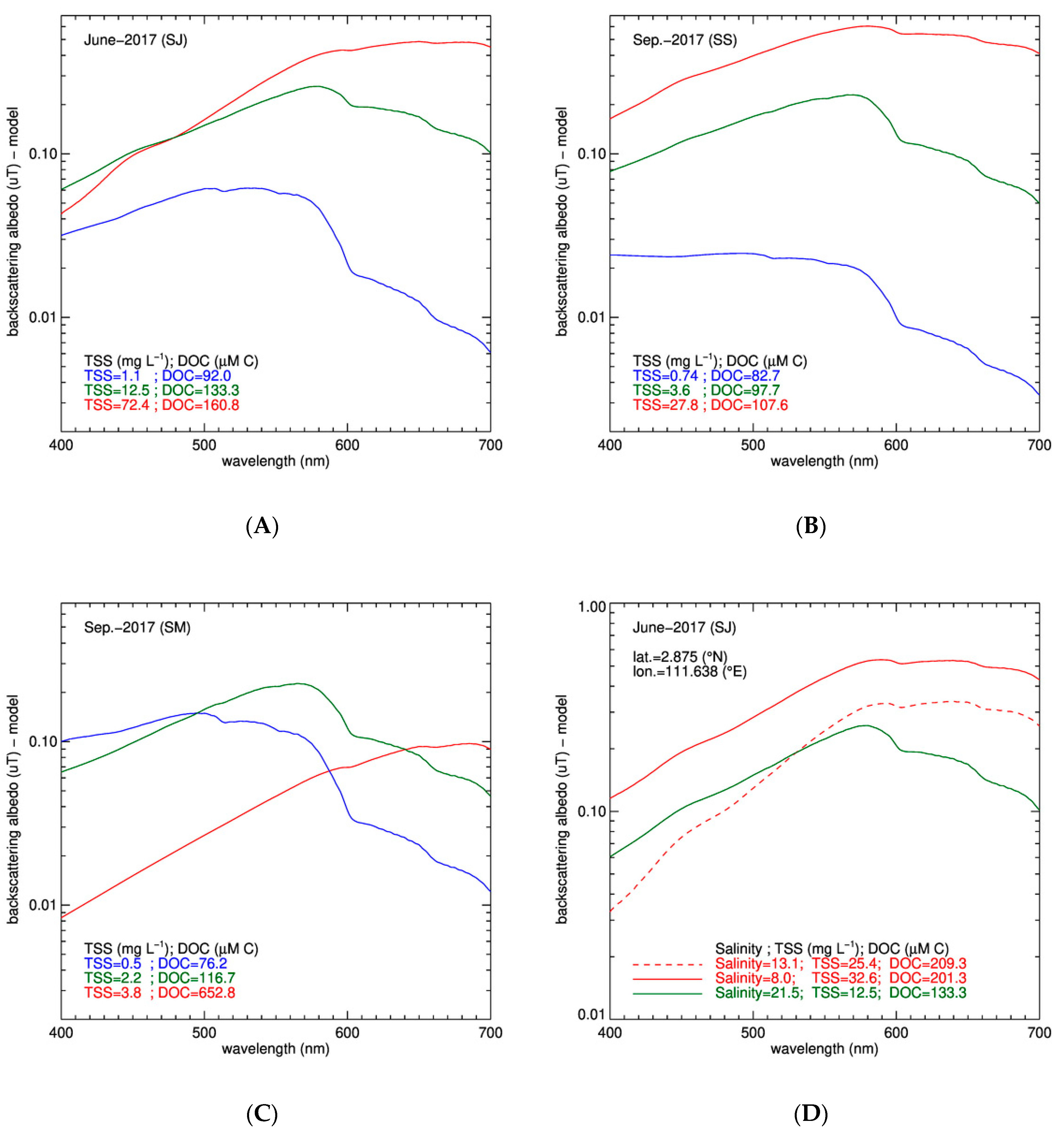
3.4. Forward Modelling of Backscattering Albedo

The forward model simulates total absorption, total backscattering and backscattering albedo spectra based on the SIOP values in the spectral library. CDOM absorption is simulated as the product of DOC-specific CDOM absorption at 440 nm and DOC concentration, and is then combined with the CDOM spectral slope to yield a simulated CDOM spectrum (Equation (3)). Particulate absorption and backscattering are simulated as the products of TSS concentration and spectral TSS-specific particulate absorption, and TSS-specific backscattering (Equations (4) and (8)). Total backscattering spectra are then computed with the particulate backscattering spectral slope and by adding the backscattering of water. Total backscattering and absorption were then used in the forward model to compute the backscattering albedo (uT(λ); Equation (9); Figure 2).

This model performed well across all water types that we sampled, with uT spectra showing peaks in the blue region (400–500 nm) for clear marine waters and shifting towards the red region (600–700 nm) in turbid coastal waters (Figure 5A–D). The range in spectral shapes of modelled uT is overall consistent with observations from eastern Borneo [79,82] and other similar tropical coastal waters, such as Singapore [90] and off the Amazon [91].

In the eastern region off the Rajang delta, both in June and September 2017, stations in relatively clear marine waters had higher uT values in the blue region (400–500 nm) due to lower concentrations of TSS and DOC (Figure 5A,B). Closer to the coast, the concentrations of TSS and DOC were higher, which reduced uT in the blue due to increased absorption by particulate and dissolved substances, and increased uT in the red region due to higher backscattering. Stations close to and in the Rajang River distributary mouths had the highest concentrations of DOC and TSS in the eastern region, and uT spectra consequently had the highest values in the red region owing to the higher backscattering values (Figure 5A,B). The forward-modelled uT in the western region (SM) showed some differences to the eastern region (Figure 5A,B versus Figure 5C). For example, in clear marine waters (solid blue lines in Figure 5), uT values were on average 22% higher in the western region (SM) than in the eastern region for similar concentrations of TSS and DOC. These higher values of uT in the western region (clear marine waters) are due to higher backscattering efficiency of particles (b_bP*(650) = 0.0157) relative to the eastern region in September (b_bP*(650) = 0.0028). In contrast, closer to river mouths (solid red line; Figure 5B,C), higher DOC concentrations in the western region reduced the uT values in the blue-green (400–600 nm) part of the spectrum while the presence of TSS resulted in high values in the red (600–700 nm).

Moreover, the shape and magnitude of uT spectra close to the river mouths changed according to hydrodynamic conditions (Figure 5D). Sarawak experiences a meso-tidal range of up to 5 m, which together with the multiple river discharges results in optically complex conditions, as also seen in coastal waters elsewhere [60,92]. In June 2017, we sampled coastal waters off the Igan distributary in the Rajang delta (2.875°N 111.638°E) over a period of 14 h to understand the influence of Igan river discharges. Initially at a salinity of 13.1, the values of TSS and DOC were 25.4 mg L⁻¹ and 209.3 µM C, which caused higher uT values in the red region (dashed red line; Figure 5D). As salinity decreased to 8 and TSS concentrations increased by 51%, uT increased across the spectrum (solid red line; Figure 5D). The river plume receded after another 10 h: salinity increased to 21.5 and TSS and DOC were reduced, such that the uT spectrum shifted to have a maximum in the green region (500–600 nm; solid green line in Figure 5D). Because our spectral library includes SIOPs from different hydrodynamic conditions encountered in Sarawak coastal waters, it thus has the ability to simulate the range of optical signatures encountered in these dynamic coastal waters.

3.5. Inversion Model

Our inversion modelling approach uses the Levenberg-Marquardt (LM) algorithm [93] to iteratively change spectral SIOPs (from SSOL) for the selected OWT, and then to adjust the concentrations of TSS and DOC in the forward model until the best fit is found between the supplied and predicted backscattering albedo (uT(λ)). Briefly, the LM algorithm is an iterative technique that locates the minimum of a multivariate function that is expressed as the sum of squares of non-linear real-valued functions [94]. As we have coupled the forward model (backscattering albedo) with the iterative mechanism of the LM, our inversion model will be referred to as iSAM (iterative semi-analytical model). We used an IDL implementation of the LM algorithm (‘MPFIT’ code available at http://purl.com/net/mpfit; [95]), which we applied to our backscattering albedo model with input data of SIOPs. LM algorithms have been successfully used with in-situ data in clear ocean waters [96], complex coastal waters [97] and also with satellite remote sensing data [98].

To test the iSAM model, we grouped the dataset according to the three field expeditions (SJ, SS and SM), which represent spatially and temporally varying conditions. We first calibrated the model with the spectral library from each data subset individually and applied it to predict TSS and DOC for the remaining two datasets by supplying the computed backscattering albedo from those datasets. We then calibrated the model with the full dataset and applied it to predict the TSS and DOC for the full dataset from the backscattering albedo, to quantify the inherent model error.

For TSS, we found that iSAM did not perform very well when the spectral library from only one data subset was used to predict TSS for the other two subsets, with either relatively large biases, mean absolute errors, or both (Figure 6A–C). Model performance was relatively better when using the spectral library from either SJ or SS to predict TSS in the other two data subsets (Figure 6A,B) and was worst when using only the spectral library from SM to predict TSS in SJ and SS (Figure 6C). These results demonstrate the limitations of extrapolating SIOP datasets between bio-optically different regions in Sarawak coastal waters, especially between the eastern and western region. Finally, when all the available SIOPs were supplied to iSAM, the retrieved values of TSS exhibited no bias and only a very small MAE (Figure 6D). The small MAE (5%) reflects the inherent error associated with the inversion modelling (iSAM) approach when retrieving TSS values in Sarawak region.

We found similar results for DOC: when applying the spectral library of just one individual data subset (SJ, SS, or SM) to predict DOC for the other two subsets, iSAM performed relatively poorly, showing large biases and MAEs (Figure 7A–C). The fact that SIOPs from SS (or SJ) could not very well predict DOC concentrations for SJ (or SS) uT spectra might suggest that there were seasonal differences in the extent of biogeochemical transformations of DOC and CDOM in the eastern region, especially from photobleaching of terrestrial CDOM [58]. However, it may well simply reflect the fact that only a limited range of bio-optical conditions were sampled during each trip, with the SJ dataset especially not capturing clearer marine waters well (Table 1). However, when the spectral library contained all available SIOPs, it retrieved concentrations of DOC with good accuracy, showing no bias and only minimal MAE. This indicates only a small inherent model error for DOC retrieval (8%). Similarly, only small errors were noted for intermediate modelling components, such as a_Y(440), a_P(440) and b_bP(650) (see Figure A1A–C). Overall, our results for DOC and TSS highlight the importance of using region- and processes-specific SIOPs in Sarawak to achieve better retrievals of TSS and DOC concentrations.

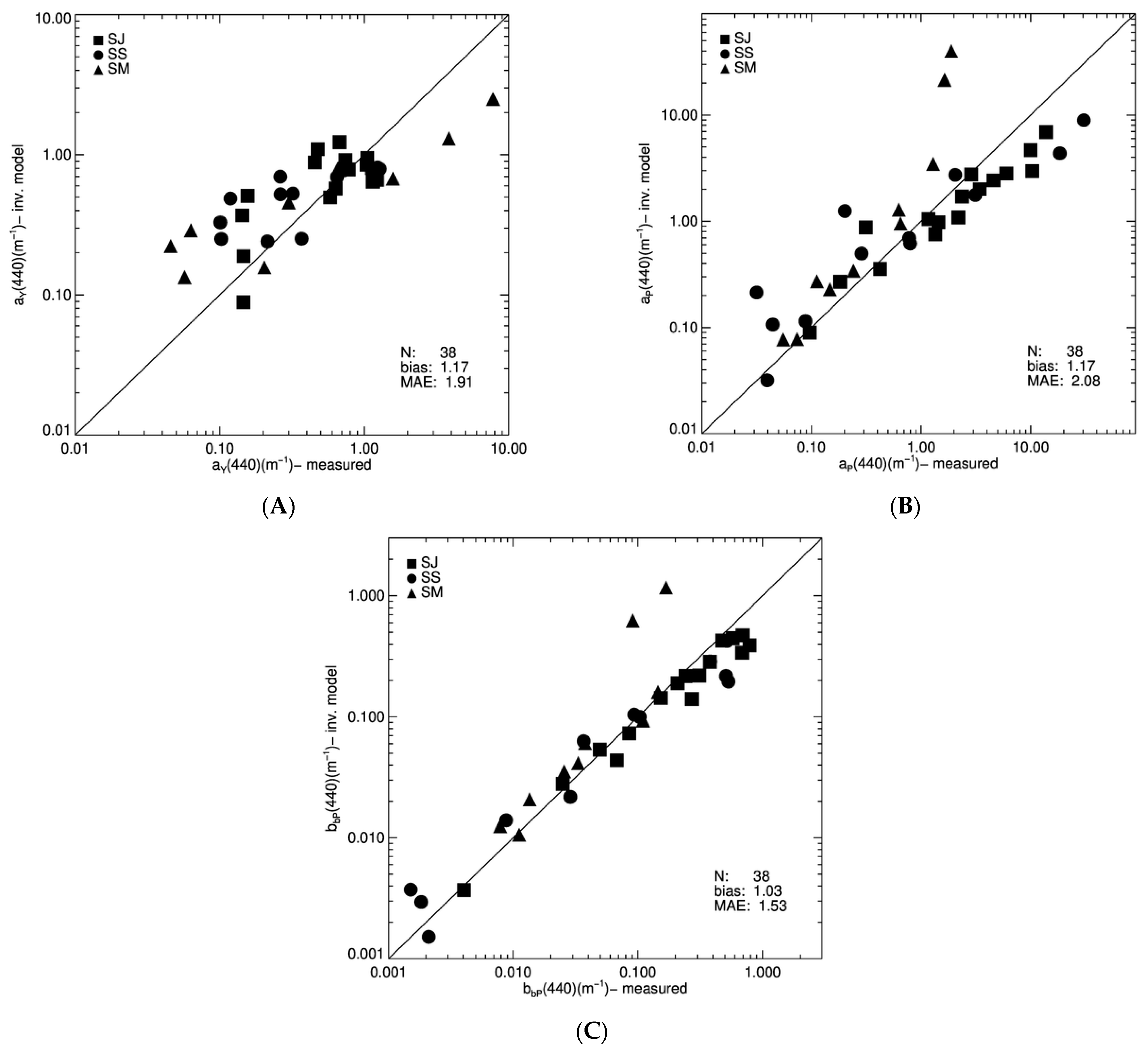
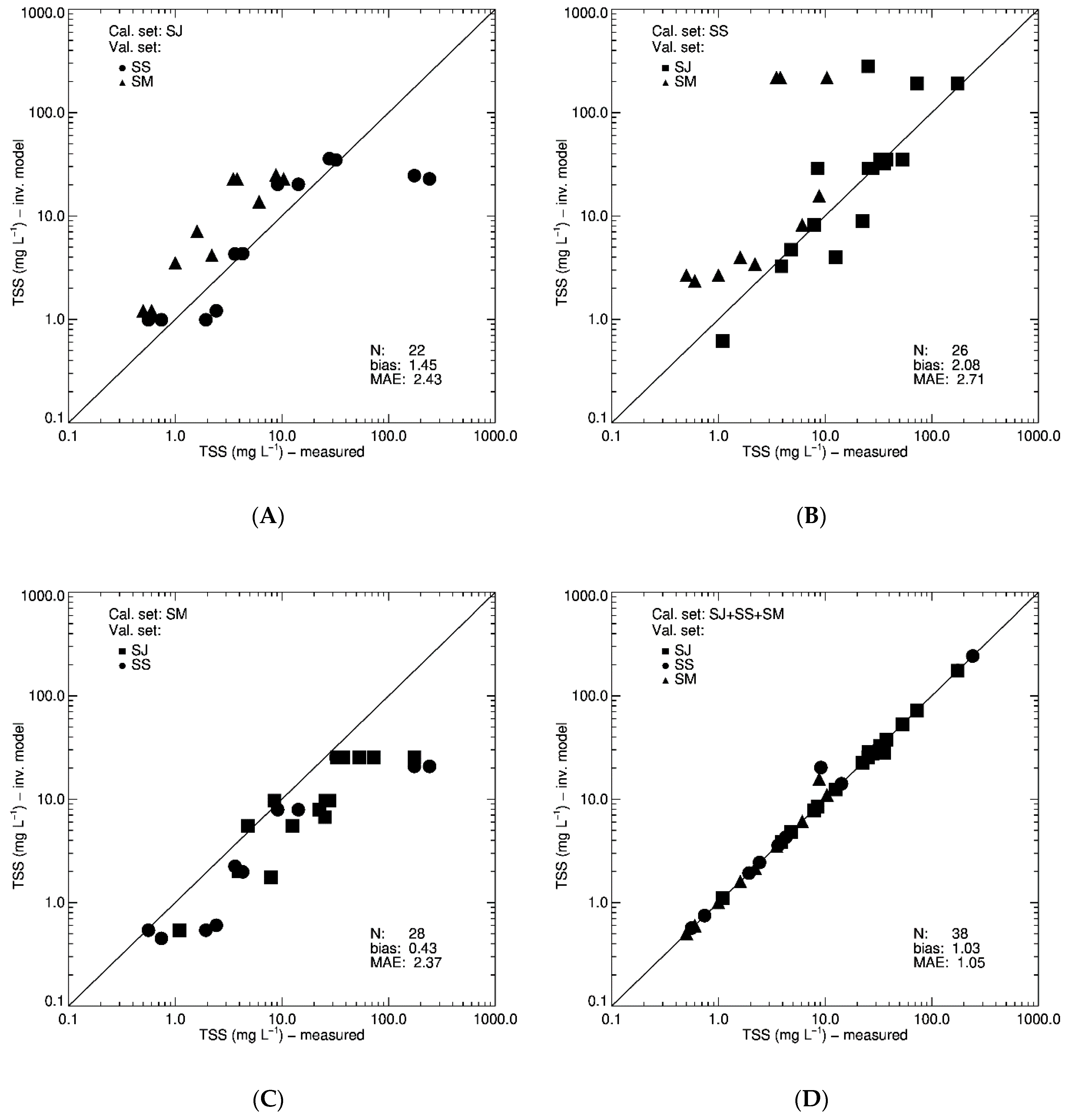
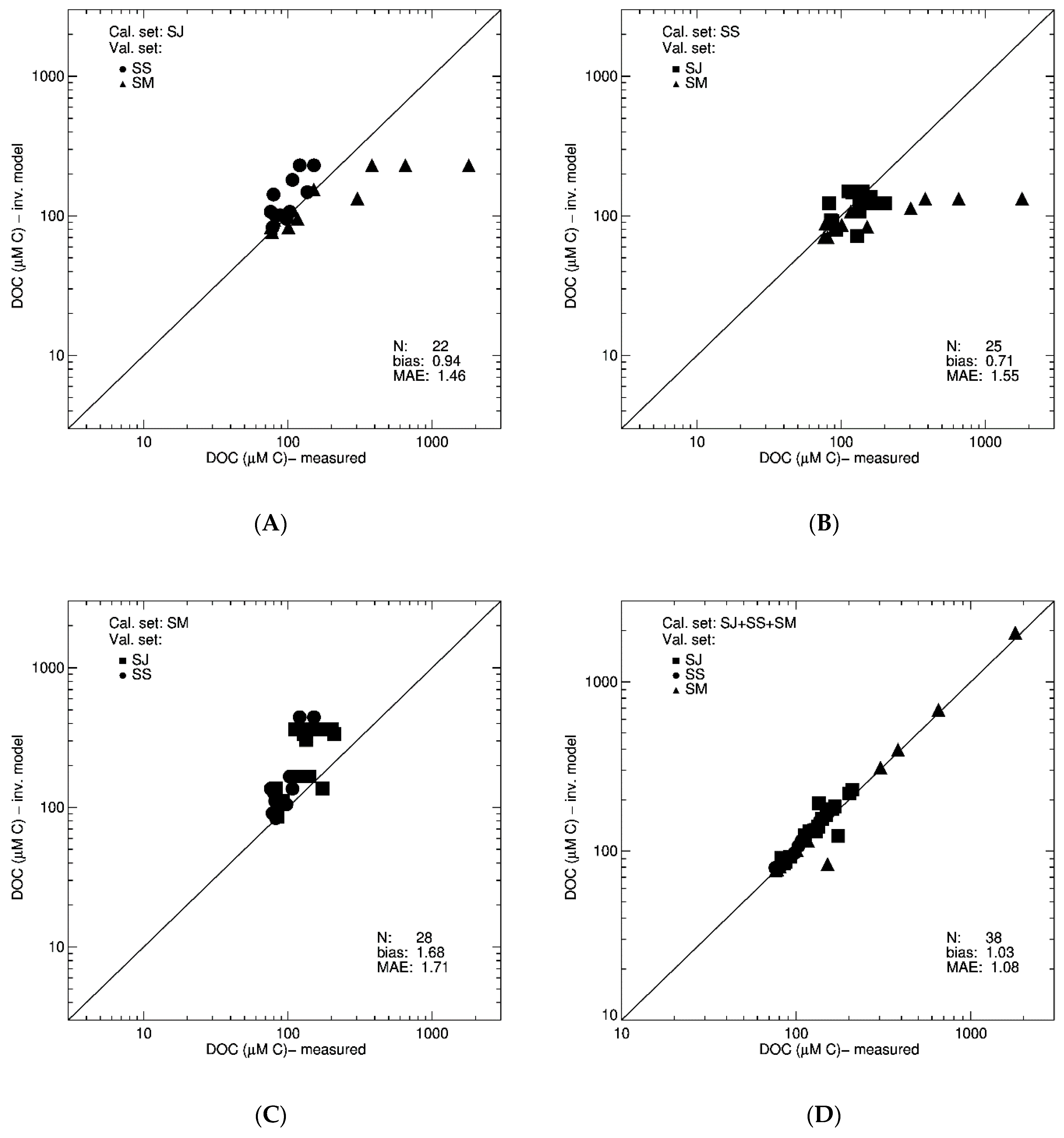
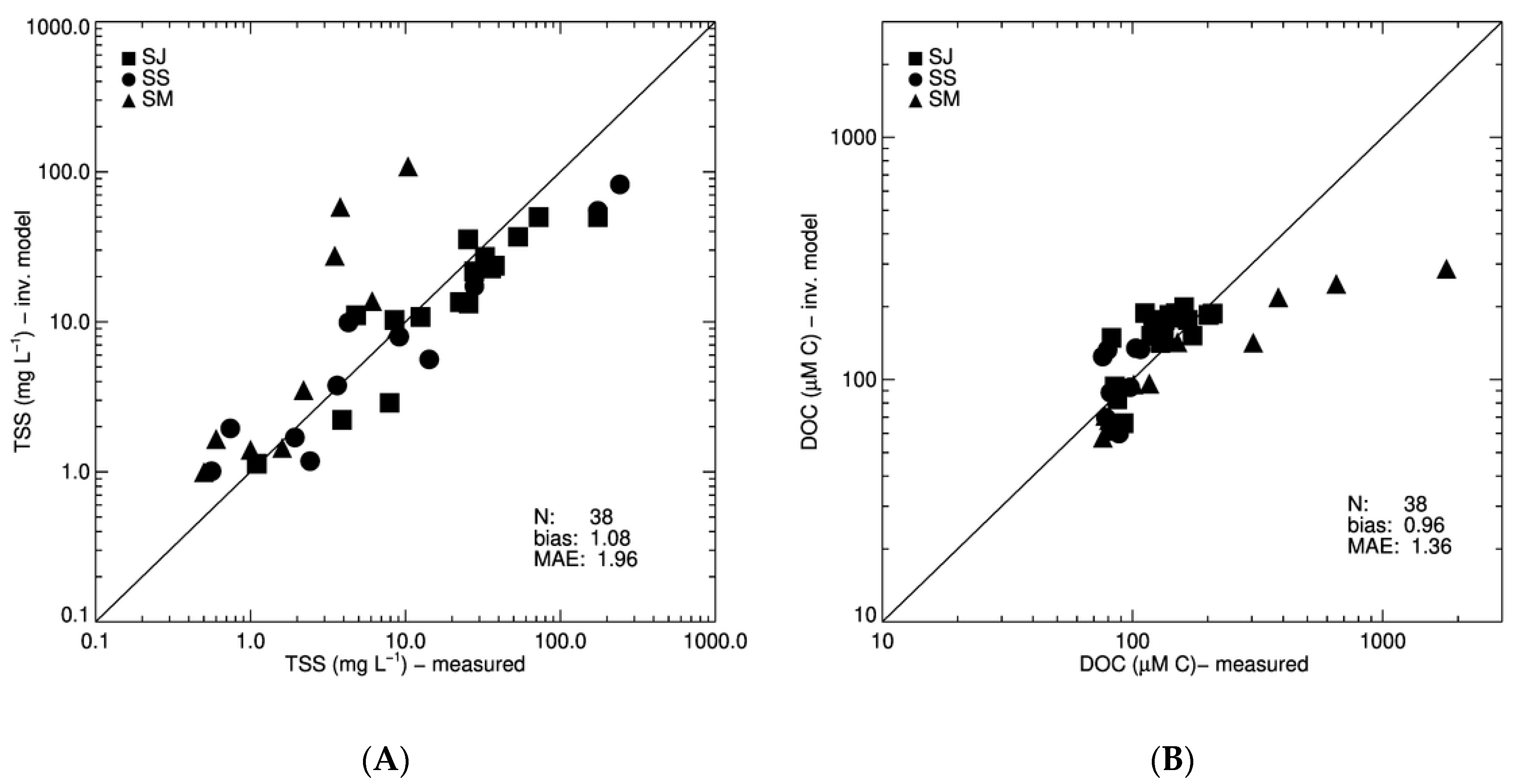
3.6. Predictive Errors of Inversion Model

We estimated the predictive error of the iSAM model using the leave-one-out cross-validation (LOO-XV) method. LOO-XV is a K-fold cross-validation technique that uses most of the data for calibration [99]. In this study, we used n−1 samples for calibration and used the left-out sample for validation. This method is repeated until all the samples have been used for validation. Measured and predicted values for each station were then used to compute the bias and MAE. These predictive errors represent the error that results if the measured biogeophysical and optical parameters for every station are predicted without using the SIOPs for that station, but instead using the SIOPs from the station with the closest-matching uT value. Since all SIOPs in the spectral library are obviously available to iSAM during normal use, the predictive errors derived from LOO-XV are almost certainly a considerable overestimate of the real errors associated with this model. However, the error estimate from LOO-XV can be taken as indicative of the errors associated with using iSAM in cases where the true SIOPs are not well represented by the existing spectral library. For cases where the true SIOPs are well matched by an SIOP combination in our spectral library, the true error is given by the inherent model error (see Figure 6D and Figure 7D) rather than by the predictive error.

The predictive error of the iSAM model for TSS estimation was low in Sarawak coastal waters (Figure 8A), when tested with in-situ optical measurements. Inversion model performance varied between subsets, with bias = 0.72 and MAE = 1.63 for SJ, and with bias = 0.76 and MAE = 1.91 for SS. However, in the SM subset the model performance was relatively poor (bias = 2.52 and MAE = 2.57), mainly due to stations in SM region that were influenced by the Samunsam river discharges. At these stations, large values of DOC (382.6, 652.8, 1798.7 µM C) were noted and the resulting average model bias was 10.78 for TSS retrieval. Stations with such high concentrations of DOC were very close to river mouths and adjacent land, and such pixels are generally flagged as problematic in remote sensing imagery anyway. In case such river discharges are transported further out to sea without dilution, then the inversion model may be limited in its performance in such pixels. iSAM performance varied in changing water conditions: in clear marine waters (TSS < 1 mg/L) the model bias was 1.83, in coastal waters (1 < TSS < 100 mg/L) the model bias was 1.06, and in highly turbid waters (TSS > 100 mg/L), iSAM under-estimated TSS values with an average bias of 0.29. Highly turbid waters with TSS concentrations above 100 mg/L were only encountered within rivers and their estuaries, but not in coastal waters beyond river mouths, so this underestimate is unlikely to affect coastal remote sensing applications of iSAM. Overall, the iSAM inversion model has good predictive error statistics in coastal waters, and relatively poor performance in clear marine waters and highly turbid river discharges. The performance of iSAM in Sarawak coastal waters could be improved by including more bio-optical measurements from clear and highly turbid waters in SSOL.

Retrieval of DOC with the iSAM model shows good agreement with DOC measurements (Figure 8B) with low predictive errors (bias = 0.96, MAE = 1.36). Consistent with the performance on the full dataset, iSAM also performed well in subsets SJ (bias = 1.09, MAE = 1.21), SS (bias = 1.21, MAE = 1.31) and SM (bias = 0.62, MAE = 1.61). The largest deviations were observed in the SM dataset for the high-DOC stations (>300 µM DOC) taken directly adjacent to the river mouth. The mismatches in DOC estimates indicate the bio-optical variability of DOC (and CDOM) present in the coastal waters along the eastern coast of Sarawak [58,84]. Comparison of iSAM performance across different DOC gradients also showed minimal predictive errors in waters with DOC < 100 µM DOC (relatively clear waters; bias = 1.10, MAE = 1.28) and for waters where 100 > DOC < 300 µM C (coastal waters; bias = 1.07 and MAE = 1.20). The highest predictive error (bias = 0.37 and MAE = 2.66) was observed for stations in highly turbid coastal waters at the river mouths. In general, iSAM thus performs well in Sarawak coastal waters for the retrieval of DOC concentrations. However, like TSS retrieval, its performance deviates in highly turbid conditions created by direct river discharges close to shore. Predictive errors associated with the IOPs are shown in Figure A2.

3.7. Limitations of the Optical Model

Figure 9 shows the limitations in extrapolating SIOP sets across different regions. In clear marine waters (relatively low concentrations of TSS), using SIOPs from other regions could lead to large deviations in the spectral shape of uT (Figure 9A). The simulated uT at station SS03 (2.11°N/110.80°E; TSS = 0.74 mg L⁻¹ and DOC = 82.7 µM C) deviated significantly (MPRD = 73.4%) when the SIOP set from similar waters of SJ11 (2.61° N/111.02° E; TSS = 1.1 mgL⁻¹ and DOC = 92 µM C) was used. Similarly, simulating SS03 with SIOPs from clear waters of the western region (SM11; 1.92° N/109.8° E) resulted in a MPRD of 485.9%, indicating that not all clear waters in Sarawak region have the same bio-optical properties. Even in coastal waters, large deviations of simulated spectra were observed both in waters with relatively higher spectral values at green (Figure 9B) and red wavelengths (Figure 9C). Figure 9D demonstrates the influence of short-term variability of SIOPs on simulated uT at the same geographic location (2.87° N/111.63° E) within just 14 h. The solid line in Figure 9D is from station SJ15 (salinity = 8.0), the dashed line indicates uT simulated using SIOPs from SJ14 (04:50 h prior to SJ15; salinity = 13.0), and the dotted line indicates SIOPs from SJ16 (09:20 h after SJ15; salinity = 21.5). This observed variability in uT indicates the changes in the bio-optical properties at this location in response to hydrodynamic conditions. The examples shown in Figure 9 demonstrate the importance of using region- and process-specific SIOPs to simulate realistic optical signatures (uT). This means that the more SIOPs from different hydrodynamic and biogeochemical conditions in Sarawak are included in SSOL, the better are the chances that iSAM will invert the signature successfully. Currently, SSOL has 38 full spectral SIOP sets. To improve the performance of bio-optical models, future studies should measure and improve the Sarawak spectral optical library.

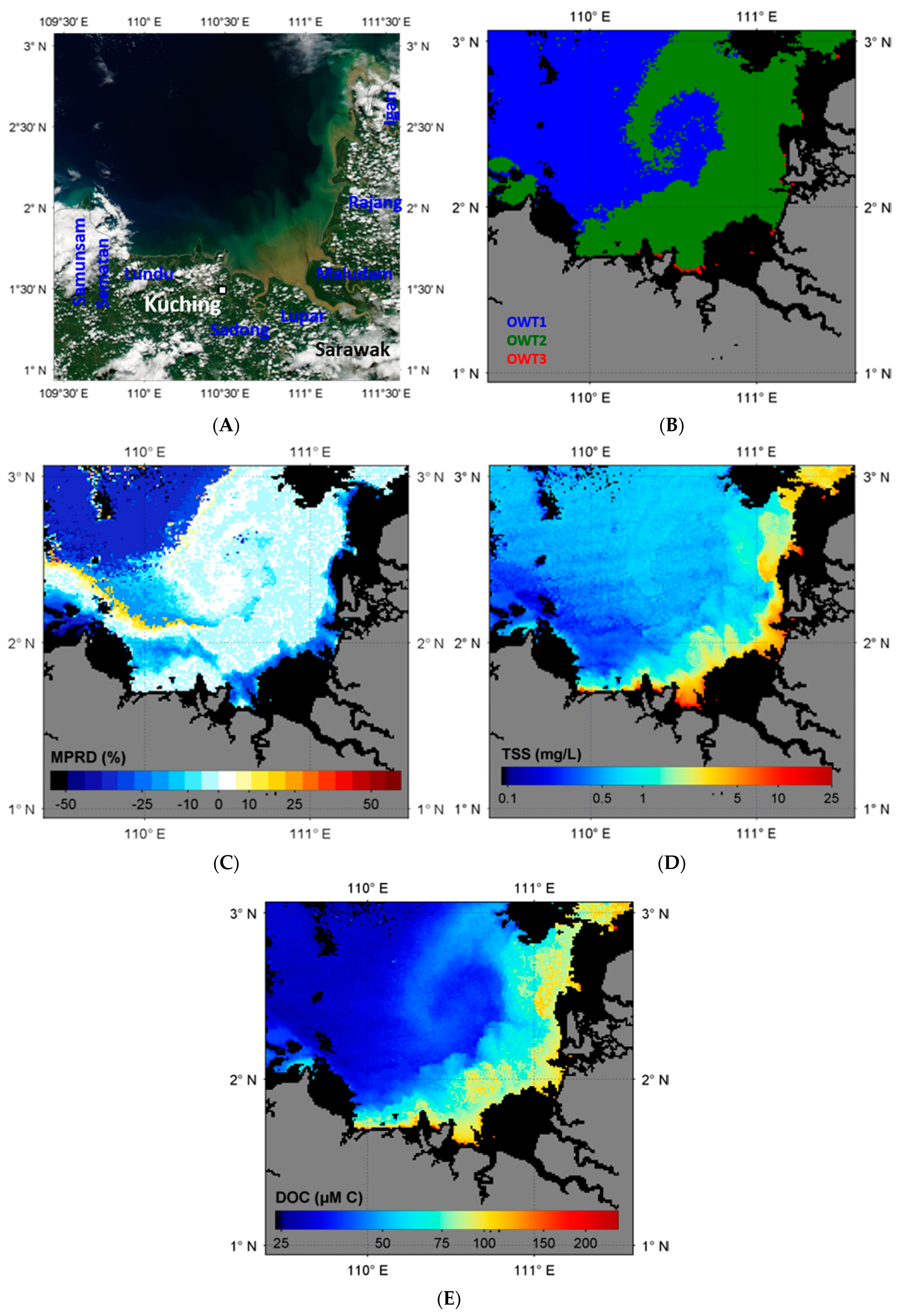
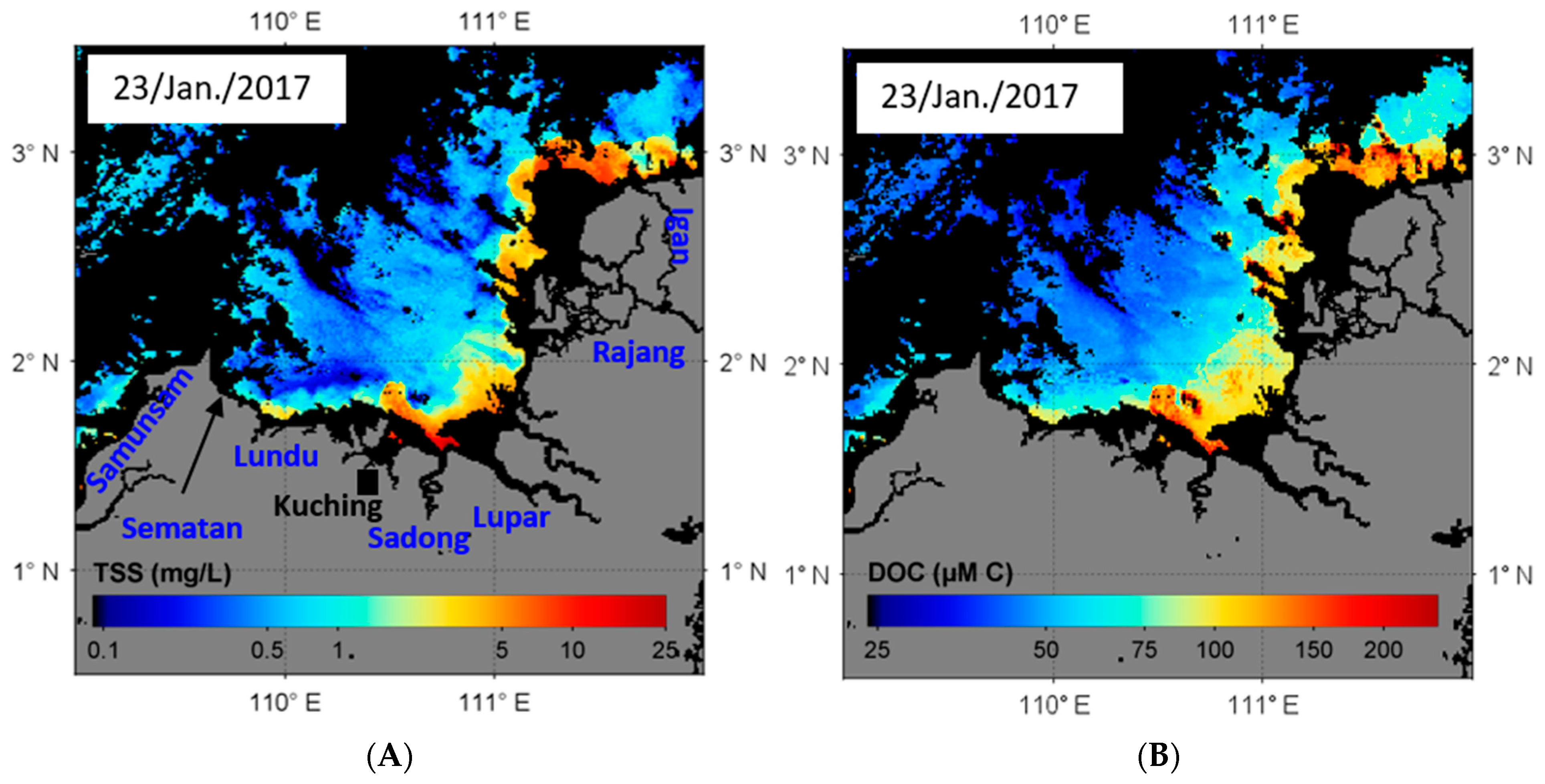
3.8. Model Application to Satellite Remote Sensing Data

To demonstrate the use of the iSAM inversion model for remote sensing purposes, we applied it to a MODIS AQUA image from 14 June 2017. Cloud cover is a major challenge for optical remote sensing in equatorial regions, and still affected some areas of this rare, largely cloud-free, image. The true-colour image (Figure 10A) shows clear blue marine waters in the South China Sea, turbid sediment-rich waters all along the coast, and turbid river discharges near multiple river mouths. Also visible is the dark DOC discharge emanating from the Maludam peatland region.

The MODIS AQUA Level 2 product that we supplied to iSAM was first converted from remote sensing reflectance at the bottom of the atmosphere to underwater remote sensing reflectance (Equation (11)) and further to backscattering albedo (uT(λ); Equation (14)). Cloud-free pixels were classified into the three optical water types (OWT, see Section 3.2) according to the reflectance signature, allowing suitable SIOPs to be selected from the spectral library and supplied to iSAM for inversion. This classification discriminated well between different water types, clearly revealing an eddy feature with river-influenced water (OWT2) moving offshore that is not evident in the true-colour image (Figure 10A,B). Also observed is the presence of highly turbid waters (OWT3) in narrow regions very close to the coast. Unfortunately, most areas with OWT3 pixels were masked in the Level 2 product due to the failure of the atmospheric correction in these waters.

Figure 10C shows the spectral matching achieved by iSAM for this MODIS Aqua image. Mean percent relative deviation (MPRD) is the mean of spectral deviations between MODIS measurements and the iSAM-simulated uT(λ). In general, iSAM achieved good agreement in most of the coastal waters (OWT2), with MPRD varying between ±10%. Relatively higher levels of model performance were achieved in OWT2 because the SSOL includes sufficient SIOP members that represent the hydrodynamic and biogeochemical conditions in Sarawak coastal waters. Closer to the land, MPRD reached up to −20%, while in clear marine water (OWT1) the model performance varied between −20 to −40%. The larger deviations observed in model performance in OWT1 indicate a lack of sufficient SIOP members representing these waters in our spectral library.

TSS and DOC concentrations derived using iSAM for the image of 14 June 2017 in coastal water types are within the range we measured (Figure 10C,D; Table 1). TSS values were relatively higher in coastal waters than compared to offshore regions, with highest values seen in pixels closer to river mouths (Rajang, Igan, Lupar, Sematan and Lundu). It is also evident from the image that the eastern coast of Sarawak had higher concentrations of TSS delivered by several rivers (e.g., Rajang and Lupar) than compared to the western coast of Sarawak. The MODIS Aqua-derived DOC concentrations showed similar patterns to TSS, with generally high values throughout the coastal waters and peak values closest to river mouths (Figure 10E). In offshore marine waters (OWT1), the model clearly under-estimates DOC concentrations, because the spectral library lacks data for CDOM-poor marine DOC that would predominate in waters unaffected by terrestrial DOC inputs. An analysis of fluorescence spectra measured in parallel with our DOC and CDOM data suggests that even in the clearest waters we sampled, 20–40% of DOC was of terrestrial origin [84], and therefore characterised by higher specific absorption than typical for marine waters. An interesting feature to note is the elevated DOC concentration in the eddy structure, which appears to carry DOC from the peatland-rich Rajang delta further into the ocean. Such remote sensing images of the distribution of DOC and TSS can supply important information for our understanding of carbon and sediment transport and processing in complex coastal ocean regions of Sarawak.

Figure 11 shows TSS and DOC estimates from MODIS Aqua for different time periods in 2017, revealing the high spatio-temporal variation in DOC and TSS in Sarawak. In these equatorial coastal waters, it was difficult to find completely cloud free images. For this demonstration purpose, we selected relatively cloud-free images from 23 January, 4 May and 21 May (all 2017). Figure 11A,B, from 23 January, show conditions during the north-east monsoon period, with generally high concentrations of TSS and DOC in coastal waters. In particular, strong river discharges carrying TSS and DOC could be observed in front of the Sadong river mouth and all across coastal waters in front of the Rajang and Igan river mouths. However, the concentrations are relatively low in coastal waters along the eastern side (Samunsam-Lundu region) of Sarawak. Figure 11C,D show MODIS images from 4 May during the early south-west monsoon period. In these two images, TSS and DOC concentrations are high all along the Sarawak coast. The higher concentrations in coastal waters could be linked to strong river discharges, especially from the Rajang delta, and the Lupar and Samunsam rivers. The Rajang and Igan along the eastern coast had higher concentrations and a wider spread of discharges compared to the rivers in the western region. Higher DOC concentrations delivered by the Samunsam river are consistent with our in-situ measurements from this blackwater river (Table 1). Similar to the image from January, the western region has the largest areal extent of waters with relatively low concentrations of TSS and DOC, indicating higher water quality. Finally, images from 21 May show higher concentrations in front of the Rajang and Igan river mouths, but a reduced spread of these high concentration features out to sea. Also, the strong river discharge with high concentrations of TSS and DOC from the Samunsam river was not present, probably owing to differences in tidal conditions during the satellite overpass.

Overall, the TSS and DOC images derived using iSAM presented in Figure 11 clearly demonstrate the strength of remote sensing maps in understanding Sarawak coastal waters. These iSAM-derived images reveal hotspots of river discharge that contribute particulate and dissolved substances to the coastal ecosystems. Figure 10E further shows that hydrodynamic processes can transport particulate and dissolved substances far into the ocean. Overall, it appears that the western region has higher water quality in terms of the concentrations of dissolved and particulate terrestrial substances, consistent with the presence of coral reefs in that region.

4. Conclusions and Future Direction

This is the first study to analyse bio-optical properties and develop a remote sensing inversion model to retrieve TSS and DOC concentrations in Sarawak, where tropical coastal waters are influenced by peatland-draining river discharges. The main results from this study are:

• Analysis of bio-optical properties showed that specific inherent optical properties of particulate and dissolved substances varied strongly across the coastal region of Sarawak.
• An optical inversion model coupled with the Sarawak spectral optical library successfully retrieved TSS and DOC concentrations from in-situ measurements of backscattering albedo.
• Remote sensing demonstration products of MODIS Aqua-derived TSS and DOC show the influence of river discharges on Sarawak coastal waters.

The bio-optical analysis presented in this study extends our understanding of coastal bio-optical properties and their variability in response to changing hydrodynamic processes. The optical model and its parameterisation will benefit both remote sensing and coastal ecosystem modelling efforts in complex coastal waters such as Sarawak. The remote sensing inversion products developed in this study now provide a synoptic view of processes affecting coastal water quality of Sarawak. New spatial and temporal remote sensing products, as demonstrated in this study, will help improve coastal monitoring practices and management strategies in Sarawak coastal waters.

This is the first study in Borneo that uses a comprehensive set of biogeochemical and optical properties. However, there are still further improvements that could help expand our understanding of coastal biogeochemical and optical dynamics in Sarawak. Expanding the Sarawak spectral library further across Borneo (e.g., into Brunei and Sabah) will help large-scale spatial studies along the western coast of Borneo. The bio-optical datasets included in SSOL currently only represent the conditions during June and September 2017, and it might improve the model solution if the SSOL is further expanded with more samples that represent the peak periods of north-east and south-west monsoons. Finally, in this study we validated the inversion model mainly with in-situ optical data. It is a challenge to achieve satellite match-ups in tropical coastal regions due to the extensive cloud cover, but it is important to attempt further validation match-ups in these waters. We therefore recommend that the local Sarawak research community should conduct further bio-optical studies to help improve satellite match-up datasets in this region.

References

1. Das, N.; Mahanta, C.; Kumar, M. Water quality under the changing climatic condition: A review of the Indian scenario. In Emerging Issues in the Water Environment during Anthropocene; Springer: Berlin/Heidelberg, Germany, 2020; pp. 31–61. [Google Scholar]
2. Fabricius, K.; De’ath, G.; McCook, L.; Turak, E.; Williams, D.M. Changes in algal, coral and fish assemblages along water quality gradients on the inshore Great Barrier Reef. Mar. Pollut. Bull. 2005, 51, 384–398. [Google Scholar] [CrossRef] [PubMed]
3. Cao, W.; Wong, M.H. Current status of coastal zone issues and management in China: A review. Environ. Int. 2007, 33, 985–992. [Google Scholar] [CrossRef] [PubMed]
4. Cooper, T.F.; Gilmour, J.P.; Fabricius, K.E. Bioindicators of changes in water quality on coral reefs: Review and recommendations for monitoring programmes. Coral Reefs 2009, 28, 589–606. [Google Scholar] [CrossRef] [Green Version]
5. Wenger, A.S.; Williamson, D.H.; da Silva, E.T.; Ceccarelli, D.M.; Browne, N.K.; Petus, C.; Devlin, M.J. Effects of reduced water quality on coral reefs in and out of no-take marine reserves. Conserv. Biol. 2016, 30, 142–153. [Google Scholar] [CrossRef] [PubMed]
6. Livingston, R.J.; McGlynn, S.E.; Niu, X. Factors controlling seagrass growth in a gulf coastal system: Water and sediment quality and light. Aquat. Bot. 1998, 60, 135–159. [Google Scholar] [CrossRef]
7. Saunders, M.I.; Leon, J.; Phinn, S.R.; Callaghan, D.P.; O’Brien, K.R.; Roelfsema, C.M.; Lovelock, C.E.; Lyons, M.B.; Mumby, P.J. Coastal retreat and improved water quality mitigate losses of seagrass from sea level rise. Glob. Chang. Biol. 2013, 19, 2569–2583. [Google Scholar] [CrossRef] [PubMed]
8. Lotze, H.K.; Lenihan, H.S.; Bourque, B.J.; Bradbury, R.H.; Cooke, R.G.; Kay, M.C.; Kidwell, S.M.; Kirby, M.X.; Peterson, C.H.; Jackson, J.B.C. Depletion, degradation, and recovery potential of estuaries and coastal seas. Science 2006, 312, 1806–1809. [Google Scholar] [CrossRef] [PubMed]
9. Schaffelke, B.; Mellors, J.; Duke, N.C. Water quality in the Great Barrier Reef region: Responses of mangrove, seagrass and macroalgal communities. Mar. Pollut. Bull. 2005, 51, 279–296. [Google Scholar] [CrossRef]
10. Cheevaporn, V.; Menasveta, P. Water pollution and habitat degradation in the Gulf of Thailand. Mar. Pollut. Bull. 2003, 47, 43–51. [Google Scholar] [CrossRef]
11. Adeyemo, O.K. Consequences of pollution and degradation of Nigerian aquatic environment on fisheries resources. Environmentalist 2003, 23, 297–306. [Google Scholar] [CrossRef]
12. Giacomazzo, M.; Bertolo, A.; Brodeur, P.; Massicotte, P.; Goyette, J.-O.; Magnan, P. Linking fisheries to land use: How anthropogenic inputs from the watershed shape fish habitat quality. Sci. Total Environ. 2020, 717, 135377. [Google Scholar] [CrossRef] [PubMed]
13. Chong, V.C.; Lee, P.K.Y.; Lau, C.M. Diversity, extinction risk and conservation of Malaysian fishes. J. Fish Biol. 2010, 76, 2009–2066. [Google Scholar] [CrossRef] [PubMed]
14. Findlay, S.E.G.; Parr, T.B. Dissolved organic matter. In Methods in Stream Ecology; Elsevier: Amsterdam, The Netherlands, 2017; pp. 21–36. [Google Scholar]
15. Bauer, J.E.; Cai, W.-J.; Raymond, P.A.; Bianchi, T.S.; Hopkinson, C.S.; Regnier, P.A.G. The changing carbon cycle of the coastal ocean. Nature 2013, 504, 61–70. [Google Scholar] [CrossRef] [PubMed]
16. Newcombe, C.P.; MacDonald, D.D. Effects of suspended sediments on aquatic ecosystems. N. Am. J. Fish. Manag. 1991, 11, 72–82. [Google Scholar] [CrossRef]
17. Dodds, W.K.; Whiles, M.R. Quality and quantity of suspended particles in rivers: Continent-scale patterns in the United States. Environ. Manag. 2004, 33, 355. [Google Scholar] [CrossRef]
18. Islam, M.S.; Tanaka, M. Impacts of pollution on coastal and marine ecosystems including coastal and marine fisheries and approach for management: A review and synthesis. Mar. Pollut. Bull. 2004, 48, 624–649. [Google Scholar] [CrossRef]
19. Wilber, D.H.; Clarke, D.G. Biological Effects of Suspended Sediments: A Review of Suspended Sediment Impacts on Fish and Shellfish with Relation to Dredging Activities in Estuaries. N. Am. J. Fish. Manag. 2001, 21, 855–875. [Google Scholar] [CrossRef]
20. Bannister, R.J.; Battershill, C.N.; De Nys, R. Suspended sediment grain size and mineralogy across the continental shelf of the Great Barrier Reef: Impacts on the physiology of a coral reef sponge. Cont. Shelf Res. 2012, 32, 86–95. [Google Scholar] [CrossRef]
21. Todd, V.L.G.; Todd, I.B.; Gardiner, J.C.; Morrin, E.C.N.; MacPherson, N.A.; DiMarzio, N.A.; Thomsen, F. A review of impacts of marine dredging activities on marine mammals. ICES J. Mar. Sci. 2015, 72, 328–340. [Google Scholar] [CrossRef] [Green Version]
22. Erftemeijer, P.L.A.; Lewis, R.R.R., III. Environmental impacts of dredging on seagrasses: A review. Mar. Pollut. Bull. 2006, 52, 1553–1572. [Google Scholar] [CrossRef]
23. Erftemeijer, P.L.A.; Riegl, B.; Hoeksema, B.W.; Todd, P.A. Environmental impacts of dredging and other sediment disturbances on corals: A review. Mar. Pollut. Bull. 2012, 64, 1737–1765. [Google Scholar] [CrossRef] [PubMed]
24. Carlson, C.A.; Hansell, D.A. DOM Sources, Sinks, Reactivity, and Budgets. In Biogeochemistry of Marine Dissolved Organic Matter, 2nd ed.; Elsevier: Amsterdam, The Netherlands, 2015; pp. 65–126. [Google Scholar]
25. Gattuso, J.-P.; Frankignoulle, M.; Wollast, R. Carbon and carbonate metabolism in coastal aquatic ecosystems. Annu. Rev. Ecol. Syst. 1998, 29, 405–434. [Google Scholar] [CrossRef] [Green Version]
26. Barrón, C.; Duarte, C.M. Dissolved organic carbon pools and export from the coastal ocean. Glob. Biogeochem. Cycles 2015, 29, 1725–1738. [Google Scholar] [CrossRef] [Green Version]
27. Lønborg, C.; Carreira, C.; Jickells, T.; Álvarez-Salgado, X.A. Impacts of Global Change on Ocean Dissolved Organic Carbon (DOC) Cycling. Front. Mar. Sci. 2020, 7, 466. [Google Scholar] [CrossRef]
28. Watanabe, K.; Kuwae, T. How organic carbon derived from multiple sources contributes to carbon sequestration processes in a shallow coastal system? Glob. Chang. Biol. 2015, 21, 2612–2623. [Google Scholar] [CrossRef] [PubMed]
29. Ward, N.D.; Bianchi, T.S.; Medeiros, P.M.; Seidel, M.; Richey, J.E.; Keil, R.G.; Sawakuchi, H.O. Where carbon goes when water flows: Carbon cycling across the aquatic continuum. Front. Mar. Sci. 2017, 4, 7. [Google Scholar] [CrossRef] [Green Version]
30. Horsburgh, J.S.; Jones, A.S.; Stevens, D.K.; Tarboton, D.G.; Mesner, N.O. A sensor network for high frequency estimation of water quality constituent fluxes using surrogates. Environ. Model. Softw. 2010, 25, 1031–1044. [Google Scholar] [CrossRef]
31. Ruhala, S.S.; Zarnetske, J.P. Using in-situ optical sensors to study dissolved organic carbon dynamics of streams and watersheds: A review. Sci. Total Environ. 2017, 575, 713–723. [Google Scholar] [CrossRef]
32. Kineke, G.C.; Sternberg, R.W. Measurements of high concentration suspended sediments using the optical backscatterance sensor. Mar. Geol. 1992, 108, 253–258. [Google Scholar] [CrossRef]
33. Rai, A.K.; Kumar, A. Continuous measurement of suspended sediment concentration: Technological advancement and future outlook. Measurement 2015, 76, 209–227. [Google Scholar] [CrossRef]
34. Earp, A.; Hanson, C.E.; Ralph, P.J.; Brando, V.E.; Allen, S.; Baird, M.; Clementson, L.; Daniel, P.; Dekker, A.G.; Fearns, P.R.C.S. Review of fluorescent standards for calibration of in situ fluorometers: Recommendations applied in coastal and ocean observing programs. Opt. Express 2011, 19, 26768–26782. [Google Scholar] [CrossRef] [PubMed] [Green Version]
35. Soja-Woźniak, M.; Baird, M.; Schroeder, T.; Qin, Y.; Clementson, L.; Baker, B.; Boadle, D.; Brando, V.; Steven, A.D.L. Particulate backscattering ratio as an indicator of changing particle composition in coastal waters: Observations from Great Barrier Reef waters. J. Geophys. Res. Oceans 2019, 124, 5485–5502. [Google Scholar]
36. Zibordi, G.; Darecki, M. Immersion factors for the RAMSES series of hyper-spectral underwater radiometers. J. Opt. A Pure Appl. Opt. 2006, 8, 252–258. [Google Scholar] [CrossRef]
37. Brando, V.E.; Lovell, J.L.; King, E.A.; Boadle, D.; Scott, R.; Schroeder, T. The potential of autonomous ship-borne hyperspectral radiometers for the validation of ocean color radiometry data. Remote Sens. 2016, 8, 150. [Google Scholar] [CrossRef] [Green Version]
38. Groom, S.B.; Sathyendranath, S.; Ban, Y.; Bernard, S.; Brewin, B.; Brotas, V.; Brockmann, C.; Chauhan, P.; Choi, J.; Chuprin, A. Satellite ocean colour: Current status and future perspective. Front. Mar. Sci. 2019, 6, 485. [Google Scholar] [CrossRef] [Green Version]
39. Gholizadeh, M.H.; Melesse, A.M.; Reddi, L. A comprehensive review on water quality parameters estimation using remote sensing techniques. Sensors 2016, 16, 1298. [Google Scholar] [CrossRef] [Green Version]
40. Matthews, M.W. A current review of empirical procedures of remote sensing in inland and near-coastal transitional waters. Int. J. Remote Sens. 2011, 32, 6855–6899. [Google Scholar] [CrossRef]
41. Odermatt, D.; Gitelson, A.; Brando, V.E.; Schaepman, M. Review of constituent retrieval in optically deep and complex waters from satellite imagery. Remote Sens. Environ. 2012, 118, 116–126. [Google Scholar] [CrossRef] [Green Version]
42. Werdell, P.J.; McKinna, L.I.W.; Boss, E.; Ackleson, S.G.; Craig, S.E.; Gregg, W.W.; Lee, Z.; Maritorena, S.; Roesler, C.S.; Rousseaux, C.S.; et al. An overview of approaches and challenges for retrieving marine inherent optical properties from ocean color remote sensing. Prog. Oceanogr. 2018, 160, 186–212. [Google Scholar] [CrossRef]
43. Werdell, P.J.; Franz, B.A.; Bailey, S.W.; Feldman, G.C.; Boss, E.; Brando, V.E.; Dowell, M.; Hirata, T.; Lavender, S.J.; Lee, Z.P.; et al. Generalized ocean color inversion model for retrieving marine inherent optical properties. Appl. Opt. 2013, 52, 2019–2037. [Google Scholar] [CrossRef]
44. Garver, S.A.; Siegel, D.A. Inherent optical property inversion of ocean color spectra and its biogeochemical interpretation: 1. Time series from the Sargasso Sea. J. Geophys. Res. Oceans 1997, 102, 18607–18625. [Google Scholar] [CrossRef]
45. Lee, Z.; Carder, K.L.; Arnone, R.A. The quasi-analytical algorithm. In Remote Sensing of Inherent Optical Properties: Fundamentals, Tests of Algorithms, and Applications; Chapter 10, IOCCG Report Number 5; International Ocean-Colour Coordinating Group: Dartmouth, NS, Canada, 2006; pp. 73–80. [Google Scholar]
46. Long, S.M. Sarawak Coastal Biodiversity: A Current Status. Kuroshio Sci. 2014, 8, 71–84. [Google Scholar]
47. White, A.T.; Aliño, P.M.; Cros, A.; Fatan, N.A.; Green, A.L.; Teoh, S.J.; Laroya, L.; Peterson, N.; Tan, S.; Tighe, S. Marine protected areas in the Coral Triangle: Progress, issues, and options. Coast. Manag. 2014, 42, 87–106. [Google Scholar] [CrossRef]
48. Miettinen, J.; Shi, C.; Liew, S.C. Land cover distribution in the peatlands of Peninsular Malaysia, Sumatra and Borneo in 2015 with changes since 1990. Glob. Ecol. Conserv. 2016, 6, 67–78. [Google Scholar] [CrossRef] [Green Version]
49. Miettinen, J.; Liew, S.C. Degradation and development of peatlands in Peninsular Malaysia and in the islands of Sumatra and Borneo since 1990. Land Degrad. Dev. 2010, 21, 285–296. [Google Scholar] [CrossRef]
50. Ling, T.-Y.; Jaafar, N.; Nyanti, L. Water and sediment quality near shrimp aquaculture farm in Selang Sibu River, Telaga Air, Sarawak, Malaysia. World Appl. Sci. J. 2012, 18, 855–860. [Google Scholar]
51. Soo, C.-L.; Ling, T.-Y.; Lee, N. Assessment of the water quality of the western boundary of Kuching Wetland National Park, Sarawak, Malaysia. Borneo J. Resour. Sci. Technol. 2015, 5, 1–10. [Google Scholar] [CrossRef] [Green Version]
52. ChunHock, S.; Cherukuru, N.; Mujahid, A.; Martin, P.; Sanwlani, N.; Warneke, T.; Rixen, T.; Notholt, J.; Müller, M. A New Remote Sensing Method to Estimate River to Ocean DOC Flux in Peatland Dominated Sarawak Coastal Regions, Borneo. Remote Sens. 2020, 12, 3380. [Google Scholar] [CrossRef]
53. Sa’adi, Z.; Shahid, S.; Chung, E.-S.; bin Ismail, T. Projection of spatial and temporal changes of rainfall in Sarawak of Borneo Island using statistical downscaling of CMIP5 models. Atmos. Res. 2017, 197, 446–460. [Google Scholar] [CrossRef]
54. Ling, T.Y.; Soo, C.L.; Sivalingam, J.R.; Nyanti, L.; Sim, S.F.; Grinang, J. Assessment of the Water and Sediment Quality of Tropical Forest Streams in Upper Reaches of the Baleh River, Sarawak, Malaysia, Subjected to Logging Activities. J. Chem. 2016, 2016. [Google Scholar] [CrossRef]
55. Pilcher, N.; Cabanban, S.A. The Status of Coral Reefs in Eastern Malaysia Global Coral Reef Monitoring Network (GCRMN) Report; Australia Institute of Marine Science: Townsville, Australia, 2000; pp. 1–81. [Google Scholar]
56. Sun, C. Riverine influence on ocean color in the equatorial South China Sea. Cont. Shelf Res. 2017, 143, 151–158. [Google Scholar] [CrossRef]
57. Tilstone, G.H.; Moore, G.F.; Sørensen, K.; Doerffer, R.; Røttgers, R.; Ruddick, K.G.; Pasterkamp, R.; Jørgensen, P.V. Protocols for the validation of MERIS products in Case 2 waters. In Proceedings of the ENVISAT MAVT Conference, Frascatti, Italy, 20–24 October 2003; pp. 20–24. [Google Scholar]
58. Martin, P.; Cherukuru, N.; Tan, A.S.Y.; Sanwlani, N.; Mujahid, A.; Müller, M. Distribution and cycling of terrigenous dissolved organic carbon in peatland-draining rivers and coastal waters of Sarawak, Borneo. Biogeosciences 2018, 15, 6847–6865. [Google Scholar] [CrossRef] [Green Version]
59. Cherukuru, N.; Dekker, A.G.; Hardman-Mountford, N.J.; Clementson, L.A.; Thompson, P.A. Bio-optical variability in multiple water masses across a tropical shelf: Implications for ocean colour remote sensing models. Estuar. Coast. Shelf Sci. 2019, 219, 223–230. [Google Scholar] [CrossRef]
60. Oubelkheir, K.; Ford, P.W.; Clementson, L.A.; Cherukuru, N.; Fry, G.; Steven, A.D.L. Impact of an extreme flood event on optical and biogeochemical properties in a subtropical coastal periurban embayment (Eastern Australia). J. Geophys. Res. Oceans 2014, 119, 6024–6045. [Google Scholar] [CrossRef]
61. Retelletti Brogi, S.; Derrien, M.; Hur, J. In-Depth Assessment of the Effect of Sodium Azide on the Optical Properties of Dissolved Organic Matter. J. Fluoresc. 2019, 29, 877–885. [Google Scholar] [CrossRef]
62. Mitchell, B.G. Algorithms for determining the absorption coefficient for aquatic particulates using the quantitative filter technique. In Proceedings of the Ocean Optics X; Spinrad, R.W., Ed.; SPIE: Bellingham, WA, USA, 1990; Volume 1302, p. 137. [Google Scholar]
63. Green, S.A.; Blough, N.V. Optical absorption and fluorescence properties of chromophoric dissolved organic matter in natural waters. Limnol. Oceanogr. 1994, 39, 1903–1916. [Google Scholar] [CrossRef]
64. Babin, M. Variations in the light absorption coefficients of phytoplankton, nonalgal particles, and dissolved organic matter in coastal waters around Europe. J. Geophys. Res. Oceans 2003, 108, 3211. [Google Scholar] [CrossRef]
65. Morel, A. Optical properties of pure water and pure sea water. In Optical Aspects of Oceanography; Jerlov, N.G., Nielsen, E.S., Eds.; Academic Press: New York, NY, USA, 1974; pp. 1–24. [Google Scholar]
66. Boss, E.; Pegau, W.S. Relationship of light scattering at an angle in the backward direction to the backscattering coefficient. Appl. Opt. 2001, 40, 5503–5507. [Google Scholar] [CrossRef]
67. Lee, Z.; Carder, K.L.; Arnone, R.A. Deriving inherent optical properties from water color: A multiband quasi-analytical algorithm for optically deep waters. Appl. Opt. 2002, 41, 5755–5772. [Google Scholar] [CrossRef]
68. Oubelkheir, K.; Clementson, L.A.; Webster, I.T.; Ford, P.W.; Dekker, A.G.; Radke, L.C.; Daniel, P. Using inherent optical properties to investigate biogeochemical dynamics in a tropical macrotidal coastal system. J. Geophys. Res. Oceans 2006, 111, 1–15. [Google Scholar] [CrossRef] [Green Version]
69. Lee, Z.-P. A model for the diffuse attenuation coefficient of downwelling irradiance. J. Geophys. Res. Oceans 2005, 110, C02016. [Google Scholar] [CrossRef]
70. Gould, R.W., Jr.; Arnone, R.A.; Sydor, M. Absorption, scattering, and, remote-sensing reflectance relationships in coastal waters: Testing a new inversion algorith. J. Coast. Res. 2001, 17, 328–341. [Google Scholar]
71. Aurin, D.A.; Dierssen, H.M. Advantages and limitations of ocean color remote sensing in CDOM-dominated, mineral-rich coastal and estuarine waters. Remote Sens. Environ. 2012, 125, 181–197. [Google Scholar] [CrossRef]
72. Mueller, J.L.; Fargion, G.S. Ocean Optics Protocols for Satellite Ocean Color Sensor Validation, Revision 3; National Aeronautics and Space Administration, Goddard Space Flight Center: Greenbelt, MD, USA, 2002; Volume 210004. [Google Scholar]
73. Lee, Z.; Carder, K.L.; Mobley, C.D.; Steward, R.G.; Patch, J.S. Hyperspectral remote sensing for shallow waters. I. A semianalytical model. Appl. Opt. 1998, 37, 6329–6338. [Google Scholar] [CrossRef]
74. Hirata, T.; Højerslev, N.K. Relationship between the irradiance reflectance and inherent optical properties of seawater. J. Geophys. Res. Oceans 2008, 113. [Google Scholar] [CrossRef] [Green Version]
75. Zibordi, G.; Berthon, J.F. Relationships between Q-factor and seawater optical properties in a coastal region. Limnol. Oceanogr. 2001, 46, 1130–1140. [Google Scholar] [CrossRef]
76. Seegers, B.N.; Stumpf, R.P.; Schaeffer, B.A.; Loftin, K.A.; Werdell, P.J. Performance metrics for the assessment of satellite data products: An ocean color case study. Opt. Express 2018, 26, 7404–7422. [Google Scholar] [CrossRef] [Green Version]
77. Bailey, S.W.; Franz, B.A.; Werdell, P.J. Estimation of near-infrared water-leaving reflectance for satellite ocean color data processing. Opt. Express 2010, 18, 7521–7527. [Google Scholar] [CrossRef]
78. Goyens, C.; Jamet, C.; Schroeder, T. Evaluation of four atmospheric correction algorithms for MODIS-Aqua images over contrasted coastal waters. Remote Sens. Environ. 2013, 131, 63–75. [Google Scholar] [CrossRef]
79. Ambarwulan, W.; Salama, M.S.; Mannaerts, C.M.; Verhoef, W. Estimating specific inherent optical properties of tropical coastal waters using bio-optical model inversion and in situ measurements: Case of the Berau estuary, East Kalimantan, Indonesia. Hydrobiologia 2011, 658, 197–211. [Google Scholar] [CrossRef] [Green Version]
80. Bowers, D.G.; Md-Suffian, I.; Mitchelson-Jacob, E.G. Bio-optical properties of east coast Malaysia waters in relation to remote sensing of chlorophyll. Int. J. Remote Sens. 2012, 33, 150–169. [Google Scholar] [CrossRef]
81. Doxaran, D.; Cherukuru, N.; Lavender, S.J. Apparent and inherent optical properties of turbid estuarine waters: Measurements, empirical quantification relationships, and modeling. Appl. Opt. 2006, 45, 2310–2324. [Google Scholar] [CrossRef] [PubMed]
82. Budhiman, S.; Suhyb Salama, M.; Vekerdy, Z.; Verhoef, W. Deriving optical properties of Mahakam Delta coastal waters, Indonesia using in situ measurements and ocean color model inversion. ISPRS J. Photogramm. Remote Sens. 2012, 68, 157–169. [Google Scholar] [CrossRef]
83. Kirk, J.T.O. Light and Photosynthesis in Aquatic Ecosystems, 3rd ed.; Cambridge University Press: Cambridge, UK, 2010. [Google Scholar]
84. Zhou, Y.; Martin, P.; Müller, M. Composition and cycling of dissolved organic matter from tropical peatlands of coastal Sarawak, Borneo, revealed by fluorescence spectroscopy and parallel factor analysis. Biogeosciences 2019, 16, 2733–2749. [Google Scholar] [CrossRef] [Green Version]
85. Ambarwulan, W.; Budhiman, S. Deriving Inherent Optical Properties from MERIS imagery and in situ measurement using quasi-analytical-algorithm. Int. J. Remote Sens. Earth Sci. 2013, 1, 454–460. [Google Scholar] [CrossRef] [Green Version]
86. Slade, W.H.; Boss, E. Spectral attenuation and backscattering as indicators of average particle size. Appl. Sci. 2015, 54, 7264–7277. [Google Scholar] [CrossRef]
87. Stramski, D.; Boss, E.; Bogucki, D.; Voss, K.J. The role of seawater constituents in light backscattering in the ocean. Prog. Oceanogr. 2004, 61, 27–56. [Google Scholar] [CrossRef]
88. Gordon, H.R.; Brown, O.B.; Evans, R.H.; Brown, J.W.; Smith, R.C.; Baker, K.S.; Clark, D.K. A semianalytic radiance model of ocean color. J. Geophys. Res. Atmos. 1988, 93, 10909–10924. [Google Scholar] [CrossRef]
89. Brando, V.E.; Dekker, A.G.; Park, Y.J.; Schroeder, T. Adaptive semianalytical inversion of ocean color radiometry in optically complex waters. Appl. Opt. 2012, 51, 2808–2833. [Google Scholar] [CrossRef]
90. Liew, S.-C.; Chia, A.S.; Lim, K.H.; Kwoh, L.K. Modeling the reflectance spectra of tropical coastal waters. In Proceedings of the Ocean Optics: Remote Sensing and Underwater Imaging; International Society for Optics and Photonics: Bellingham, WA, USA, 2002; Volume 4488, pp. 248–255. [Google Scholar]
91. Froidefond, J.-M.; Gardel, L.; Guiral, D.; Parra, M.; Ternon, J.-F. Spectral remote sensing reflectances of coastal waters in French Guiana under the Amazon influence. Remote Sens. Environ. 2002, 80, 225–232. [Google Scholar] [CrossRef]
92. Cherukuru, N.; Brando, V.E.; Schroeder, T.; Clementson, L.A.; Dekker, A.G. Influence of river discharge and ocean currents on coastal optical properties. Cont. Shelf Res. 2014, 84, 188–203. [Google Scholar] [CrossRef]
93. Marquardt, D.W. An algorithm for least-squares estimation of nonlinear parameters. J. Soc. Ind. Appl. Math. 1963, 11, 431–441. [Google Scholar] [CrossRef]
94. Press, W.H.; Teukolsky, S.A.; Vetterling, W.T.; Flannery, B.P. Numerical Recipies in C. Error, Accuracy, and Stability; Cambridge University Press: Cambridge, UK, 1992. [Google Scholar]
95. Markwardt, C.B. Non-linear least squares fitting in IDL with MPFIT. arXiv 2009, arXiv:0902.2850. [Google Scholar]
96. Roesler, C.S. Spectral beam attenuation coefficient retrieved from ocean color inversion. Geophys. Res. Lett. 2003, 30, 1–4. [Google Scholar] [CrossRef] [Green Version]
97. Zhang, M.; Tang, J.; Dong, Q.; Song, Q.; Ding, J. Retrieval of total suspended matter concentration in the Yellow and East China Seas from MODIS imagery. Remote Sens. Environ. 2010, 114, 392–403. [Google Scholar] [CrossRef]
98. Maritorena, S.; Siegel, D.A.; Peterson, A.R. Optimization of a semianalytical ocean color model for global-scale applications. Appl. Opt. 2002, 41, 2705–2714. [Google Scholar] [CrossRef]
99. Welham, S.J.; Gezan, S.A.; Clark, S.J.; Mead, A. Statistical Methods in Biology: Design and Analysis of Experiments and Regression; CRC Press: Boca Raton, FL, USA, 2014; ISBN 1439898057. [Google Scholar]
Figure 1. Map of Sarawak indicating the spatial extent of field sampling during June and September 2017.
Remotesensing 13 00099 g001
Figure 2. Flow chart of the optical remote sensing inversion approach.
Remotesensing 13 00099 g002
Figure 3. Specific inherent optical properties included in the Sarawak spectral optical library. (A) TSS-specific particulate absorption, (B) DOC-specific absorption due to CDOM and (C) TSS-specific particulate backscattering.
Remotesensing 13 00099 g003aRemotesensing 13 00099 g003b
Figure 4. Conversion of underwater remote sensing reflectance to backscattering albedo. Comparison of in-situ measurements with model according to (A) Gordon et al., 1988, (B) Lee et al., 2002, (C) Aurin et al., 2002 using spectral f/Q values and (D) our Sarawak regional parametrisation.
Remotesensing 13 00099 g004
Figure 5. Variability of backscattering albedo in Sarawak coastal waters. (A) spectral variability during June 2017 along the eastern coast of Sarawak, (B) spectral variability during September 2017 along the eastern coast of Sarawak, (C) spectral variability during September 2017 along western coast of Sarawak (off Samunsam and Sematan river mouths) and (D) changes in spectral shape of backscattering albedo under the influence of river discharges along the eastern coast of Sarawak during June 2017.
Remotesensing 13 00099 g005
Figure 6. Performance of the optical inversion model for TSS retrieval with changing input members (Calibration set) included in the Sarawak spectral optical library. (A) Retrieval comparisons against SS and SM, (B) comparisons against SJ and SM, (C) comparisons against SJ and SS, and (D) comparisons when both the calibration and validation datasets included all available SIOP datasets in SSOL.
Remotesensing 13 00099 g006
Figure 7. Performance of the optical inversion model for DOC retrieval with changing input members (Calibration set) included in the Sarawak spectral optical library. (A) Retrieval comparisons against SS and SM, (B) comparisons against SJ and SM, (C) comparisons against SJ and SS, and (D) comparisons when both the calibration and validation datasets included all available SIOP datasets in SSOL.
Remotesensing 13 00099 g007
Figure 8. Predictive error estimates of optical inversion model using the leave-one-out cross validation method. (A) TSS retrieval comparisons and (B) DOC retrieval comparisons with uT measurements as an input to the inversion model.
Remotesensing 13 00099 g008
Figure 9. Model simulations show the limitation of extrapolating optical properties in Sarawak coastal waters. (A) comparison of optical spectra in relatively clear waters with higher values in the blue-green region, (B) comparison of optical spectra in coastal waters with a maximum in the green region of the spectrum, (C) comparison of optical spectra in turbid coastal waters with higher values in the green-red region of the spectrum, and (D) variability in optical spectral shape and magnitude due to varying SIOPS in response to changing salinity (river discharges).
Remotesensing 13 00099 g009
Figure 10. Demonstration of the optical inversion model applied to MODIS Aqua. (A) True-colour image of MODIS Aqua from 14 June 2017, (B) optical waters types detected in Sarawak coastal waters, (C) mean percent relative deviation between backscattering albedo (uT) observed by MODIS Aqua and simulated using the our Sarawak optical inversion model (iSAM), and spatial maps of (D) TSS and (E) DOC concentrations estimated using iSAM.
Remotesensing 13 00099 g010
Figure 11. Temporal variability in TSS and DOC concentrations across Sarawak coastal waters as observed by MODIS Aqua. (A,B) Spatial maps of TSS and DOC for 23 January 2017, representing north-east monsoon conditions. Higher concentrations of TSS and DOC are observed in the river plumes in front of the Rajang, Lupar and Sadong rivers. (C,D) Spatial maps for 4 May 2017 (south-west monsoon conditions) show strong river discharges near the Samunsam and Sematan rivers in the western coastal waters of Sarawak, with higher magnitudes of TSS and DOC discharged into the coastal waters. (E,F) Spatial maps for 21 May 2017 show higher concentrations of TSS and DOC discharged into coastal waters by the Igan and Rajang river mouths, and relatively clear waters over a wide region across the western part of coastal Sarawak.
Remotesensing 13 00099 g011aRemotesensing 13 00099 g011b