Abstract
Remote sensing offers a way to map crop types across large spatio-temporal scales at low costs. However, mapping crop types is challenging in heterogeneous, smallholder farming systems, such as those in India, where field sizes are often smaller than the resolution of historically available imagery. In this study, we examined the potential of relatively new, high-resolution imagery (Sentinel-1, Sentinel-2, and PlanetScope) to identify four major crop types (maize, mustard, tobacco, and wheat) in eastern India using support vector machine (SVM). We found that a trained SVM model that included all three sensors led to the highest classification accuracy (85%), and the inclusion of Planet data was particularly helpful for classifying crop types for the smallest farms (<600 m2). This was likely because its higher spatial resolution (3 m) could better account for field-level variations in smallholder systems. We also examined the impact of image timing on the classification accuracy, and we found that early-season images did little to improve our models. Overall, we found that readily available Sentinel-1, Sentinel-2, and Planet imagery were able to map crop types at the field-scale with high accuracy in Indian smallholder systems. The findings from this study have important implications for the identification of the most effective ways to map crop types in smallholder systems.
1. Introduction
Smallholder farming comprises 12% of global agricultural lands and produces approximately 30% of the global food supply [1,2]. Smallholder systems are being challenged by environmental change, including climate change and natural resource degradation [3,4]. Mapping agricultural land cover and land use change (LCLUC) is critically important for understanding the impacts of environmental change on agricultural production and the ways to enhance production in the face of these changes [5,6]. While remote sensing has been widely used to map agricultural LCLUC across the globe, it has historically been challenging to map smallholder agricultural systems given the small size of fields (<2 ha) relative to long-term, readily available imagery, such as Landsat and MODIS [7]. Over the last decade, however, new readily available sensors, including Sentinel-1, Sentinel-2, and Planet, have been launched and can provide higher-resolution datasets (<=10 m). These new sensors have been shown to better detect field-level characteristics in smallholder systems [8,9], and they have the potential to provide the critical datasets needed to improve food security over the coming decades.
One key dataset for monitoring LCLUC in smallholder systems is crop type. This is because identifying crop types is an important precursor to mapping agricultural production, particularly yield [9], and studies have shown that crop switching is one of the main axes of adaptation to environmental changes in smallholder systems [10,11]. Yet, to date, relatively little work has been carried out to map crop types in smallholder systems compared to other agricultural characteristics, such as cropped area and yield. The work that does exist to map smallholder crop types using readily available imagery has largely focused on using Sentinel 1 and 2 [9,12,13,14], yet it is likely that micro-satellite data could improve classification accuracies given their higher spatial resolution, which reduces the effect of mixed pixels at field edges [15]. To the best of our knowledge, only two studies have examined the benefits that Planet micro-satellite data provide when mapping smallholder crop types, and these two studies were conducted in Africa [16,17]. To date, no work, to the best of our knowledge, has examined the ability of Planet satellite data to map crop types in India, which is the world’s largest nation of smallholder farms [2].
In this study, we used radial kernel support vector machine (SVM) to map the crop types of smallholder farms in two sites in eastern India. We focused on using SVM because previous studies have suggested that it produces higher classification accuracies compared to other commonly used algorithms, including random forest, for supervised pixel-based classifications [18]. We specifically focused on mapping four major crops (maize, mustard, tobacco, and wheat) planted during the dry winter season in Bihar, India. We used these data to ask three specific research questions:
- How accurately do Sentinel-1, Sentinel-2, and PlanetScope imagery map crop types in smallholder systems? Which sensor or sensor combinations lead to the greatest classification accuracies?
- Does crop type classification accuracy vary with farm size? Does adding Planet satellite data improve the classification accuracy more for the smallest farms?
- How does classification accuracy vary based on the timing of imagery used? Are there particular times during the growing season that lead to a better discrimination of crop types?
This study provides important insights into the ability of new, higher-resolution satellite data to map crop types in smallholder systems in India. Such information is critical given that readily available crop type maps do not exist across the country, and crop type information can be used to better understand the impacts of environmental change in this globally important agricultural region.
2. Materials and Methods
2.1. Data
2.1.1. Study Area and Field Polygons
Our study area covered a 20 km × 20 km region in the Vaishali and Samastipur districts of Bihar in India (Figure 1), for which crop type information from 385 farms across 30 villages was collected during the winter growing season of 2016–2017. The farms sampled included four major crop types in this region: maize, mustard, tobacco, and wheat, which are sown in late November through December and are harvested from March to April.
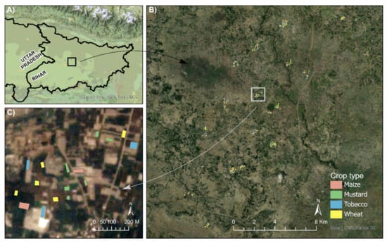
Figure 1.
(A) Study region in Bihar in eastern India. (B) Distribution of sample fields overlaid on the ArcGIS base map (ESRI Inc.). (C) Zoomed-in image of one village shown on Planet imagery acquired on 18 February 2017.
We acquired a sample of crop types across the study region based on field accessibility and to ensure adequate representation across the four main crop types; this likely resulted in the oversampling of minor crops that were planted on the least amount of area. We excluded any fields where more than one crop was planted within the same field. Farm locations were collected using Garmin E-Trex GPS units. For each farm, we recorded the geographic coordinates of the four corners and the center of the field, crop type, farmer name, and village name.
The GPS coordinates of farm boundaries obtained from the field survey were imported into ArcGIS (version 10.6.1) as a point shapefile and were overlaid on the ArcGIS base imagery. Based on the coordinates of the four corners of the fields, farm polygons were digitized manually by checking visible farm boundaries on the ArcGIS base imagery and the Google Earth Pro (https://www.google.com/earth/versions/#earth-pro, accessed on 15 March 2018) images closest to December 2016 (the date when polygons were collected). We kept the 324 polygons with clear and accurate field boundaries according to the visual interpretation of high-resolution imagery, and we did not include 61 polygons for which the farm boundaries could not be clearly identified.
2.1.2. Satellite Data
We utilized multi-temporal data from two optical sensors, Planet and Sentinel-2, and one radar sensor, Sentinel-1, that fell within our study period (15 November 2016, to 20 April 2017). We used the Google Earth Engine platform (GEE; [19]) to download preprocessed Sentinel-1 Ground Range Detected (GRD) and Sentinel-2 level-1C Top Of Atmosphere (TOA) reflectance data covering our study area. GEE uses the Sentinel-1 Toolbox (https://sentinel.esa.int/web/sentinel/toolboxes/sentinel-1, accessed on 1 April 2018) to preprocess Sentinel-1 images to generate calibrated, ortho-corrected estimates of decibels via log scaling. In addition, thermal noise removal, radiometric calibration, and terrain correction were performed using a digital elevation model (DEM) from the Shuttle Radar Topography Mission (SRTM) or the Advanced Spaceborne Thermal Emission and Reflection Radiometer (ASTER). We used all 17 Sentinel-1 GRD scenes with both VV (vertical transmit/vertical receive) and VH (horizontal transmit/horizontal receive) bands available for the 2016–2017 winter growing season (Figure 2).
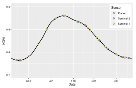
Figure 2.
Image acquisition dates for the three sensors during the 2016–2017 winter growing season plotted against average NDVI values produced using MODIS satellite imagery for our study region.
We also used all six cloud and haze-free Sentinel-2 multispectral TOA data available for the growing season (Figure 2); cloud and haze-free imagery were identified visually given that only 13 images were available throughout the growing season. We conducted atmospheric correction of all Sentinel-2 multispectral TOA bands using the Py6S package [20], which is based on the 6S atmospheric Radiative Transfer Model [21], to derive the surface reflectance for the visible (blue, green, and red at 10 m), NIR (10 m), red-edge (20 m), and SWIR (20 m) bands. In addition, based on the available literature, we derived eight spectral indices (seven from Sentinel-2 and one from Sentinel-1) that are known to capture distinct plant characteristics to improve crop classification accuracies (Table 1). We resampled all Sentinel-1 and Sentinel-2 scenes to 3 m (the spatial resolution of PlanetScope imagery) using nearest-neighbor assignment in ArcGIS software.

Table 1.
Spectral indices used in this study.
We accessed all available cloud-free Planet surface reflectance data (PlanetScope AnalyticMS level 3B product) covering our study region and period (Figure 2) through Planet’s API [31]; we similarly identified cloud-free scenes via the visual interpretation of imagery. Each image was also visually inspected for any geo-referencing errors by overlaying Planet images over the base satellite imagery in ArcGIS. As band values from Planet were not comparable with those from Sentinel-2, likely due to differences in sensor characteristics, atmospheric correction methods, and the relatively poor quality of surface reflectance correction for Planet [32], we performed histogram stretching of Planet and Sentinel-2 surface reflectance data using methods from Jain et al. [15]. Specifically, we linearly transformed histograms of each Planet band to match histograms of the same bands from Sentinel-2 images. For this correction, we used Sentinel-2 data from the date that was closest to the date of the Planet imagery. If there was no Sentinel-2 image that was within a few days of the Planet date, we took the inverse distance-weighted value between the closest Sentinel-2 dates before and after the Planet image date following methods from Jain et al. [15]. After histogram matching, both Sentinel-2 and Planet NDVI showed similar values and a consistent phenology (Figure 3). The 15 November 2016 Planet scene did not cover our entire study area, including 47 of the reference polygons. To keep all analyses constant across sensors, we removed these 47 polygons from all remaining analyses, reducing the final number of polygons used to 277.
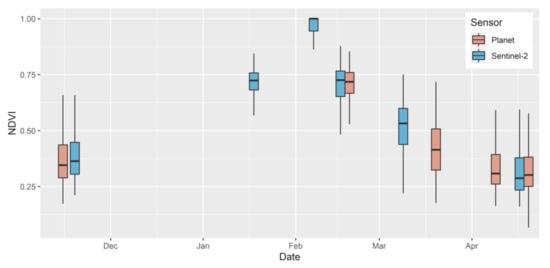
Figure 3.
NDVI values of all pixels within the reference polygons from Planet and Sentinel-2 imagery after histogram matching Planet data.
We stacked all available image dates from the resampled Sentinel-1 (3 m), resampled Sentinel-2 (3 m), and Planet (3 m) datasets, and we extracted all bands for all pixels that fell within each of the 277 polygons. This final dataset is available as a supplementary file (Supplementary Data).
2.2. Methods
2.2.1. Sampling Strategy and Feature Selection for Model Development
The reference polygons were divided into training (70%) and testing (30%) polygons stratified across crop type and field size. We stratified our training and testing polygons because we were interested in evaluating how well our models performed across crop types and field sizes. For training data, for each crop type, we selected 1893 pixels, which was the number of pixels available across all training polygons for the smallest crop type class (i.e., mustard); these pixels were selected randomly across all training polygons for each of the other three crop types. By selecting the same number of training pixels across each crop type, we ensured that each crop type was equally represented in the model. All pixels within the testing polygons were considered as the test sample. We extracted all band values and indices for all sensors and image dates for all training and test pixels using the raster package [33] in R project software [34]. Before training the SVM, we removed redundant (correlated) features following a simple correlation-based filter approach using a cutoff value of 0.9 using the caret package [35] in R project software [33]. The selected number of final input features ranged from 31 to 147 depending on the combination of sensors under consideration (Table 2).
Table 2.
The number of final input features for developing the SVM model.
2.2.2. Performance of Different Sensor Combinations
We ran the SVM using the caret package [34] in R project software [33] using a grid search along with 10-fold cross-validation to appropriately tune the gamma and cost parameters based on the training data. We then ran the SVM for each sensor and all sensor combinations (research question 1). The performance of each model was compared by examining the overall accuracy, producer/user accuracies, and crop-specific F1 scores that combined both producer and user accuracies using the harmonic mean [32].
F1 score = 2 * (Producer’s accuracy * User’s accuracy)/(Producer’s accuracy + User’s accuracy)
The SVM model that produced the best results (highest overall accuracy and F1 scores for most crops) was used in the further analysis for the remaining research questions. We found this to be the SVM model that was run using all three sensors (Section 3.1).
2.2.3. Classification Accuracy Based on Farm Size
To understand how classification accuracy varies with farm size, we examined the classification accuracy of small (<600 m2, n = 135) versus large (>=600 m2, n = 142) farms (Figure 4). We used 600 m2 to differentiate between small versus large farms because this value approximated the median value of farm sizes (627 m2) for all crops. We ran the SVM algorithm on the three-sensor dataset, as well as a two-sensor model using Sentinel-1 and Sentinel-2, to assess whether the addition of Planet data improved crop classification accuracies, particularly for small fields (research question 2).
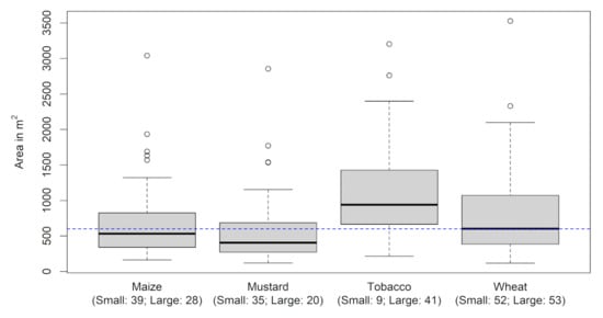
Figure 4.
Farm sizes based on crop types. The x-axis labels also show the number of small and large farms based on the 600 m2 threshold (dotted horizontal line) obtained from the field survey.
2.2.4. Classification Accuracy and Image Sampling Dates
To assess whether certain periods of crop growth were more important for improving classification accuracies (research question 3), we ran the SVM model on different subsets of input datasets based on the stages of crop growth within the growing season (Table 3). These subsets include dates from the early, peak, and late growing seasons, identified using crop phenology (Figure 2) and local knowledge. For each crop growth stage, we selected one image from each sensor that was close in date to reduce the confounding effect of increased temporal information provided when using images from multiple sensors. We compared SVM classification accuracies when using images from only one season and for all season combinations (Table 3).
Table 3.
Image acquisition dates in month and day (mmdd) within different growth stage periods during the 2016–2017 winter growing season (November to April) for all three sensors.
3. Results
3.1. Crop Classification Accuracies from a Combination of Different Sensors
Considering research question 1, the highest overall accuracy (0.85) was yielded when all three sensor datasets were combined ( Table 4 and Table S1). For individual sensors, Planet resulted in the highest classification accuracy, though this was only moderately better than that using Sentinel-2 data, and Sentinel-1 resulted in the lowest classification accuracy (Table 4). The accuracies increased as more sensors were added into the model, with the biggest increase occurring between the one-sensor and two-sensor models (Table 4).
Table 4.
Comparison of overall classification accuracies using each sensor and all sensor combinations.
Considering the best model (the three-sensor model), the F1 scores varied across crop type (Table 5), with the highest accuracies for wheat and tobacco. A major source of classification error appeared to come from the omission of mustard pixels, as indicated by the lower F1 scores and producer accuracies for the crop (Table 5 and Table S1).
Table 5.
Crop-specific F1 scores from the model using all three sensors.
3.2. The Influence of Farm Size on Classification Accuracy
For research question 2, we found that the classification accuracies were higher for pixels within large farms (600 m2) compared to those within small farms (600 m2) (Table 6 and Tables S2–S5). Notably, including data from Planet appeared to improve the crop classification of smaller farms more significantly than that of larger farms (Table 6). For example, when Planet data were combined with the other two sensors, the overall classification accuracy increased by almost 6% for small farms compared to around 4% for larger farms. Planet data also generally increased the crop-specific F1 scores (Table 6), including producer’s and user’s accuracies, except for the producer’s accuracy of tobacco (Tables S2–S5). Overall, these results suggest that including Planet data improves the classification accuracy, particularly for small farms.
Table 6.
Classification accuracies for the test pixels from the large and small farms before and after including Planet data with the combined Sentinel-1 and Sentinel-2 data.
3.3. Classification Accuracies Based on Images from Different Periods of the Growing Season
Considering research question 3, we found that the late season (i.e., late-March to mid-April) led to the highest classification accuracy (0.67) when the three-sensor SVM was run separately using images from one of the three stages of the growing period (early, peak, and late, Figure 5, Tables S6–S11). The overall accuracy and F1 scores for all four crops were quite low when only early-season images were used (Figure 5). The time period that resulted in the highest accuracy varied based on crop type. The F1 scores for mustard and tobacco were highest when using peak-season images, while the F1 scores were highest when using late-season images for maize and wheat. This was likely due to differences in phenologies and harvest dates across crops (Figure 6). Generally, the classification accuracies improved as more growing seasons were considered in the model, though adding early-season images did not improve the model fit compared to only using peak and late-season images (Figure 5, Tables S6–S11).
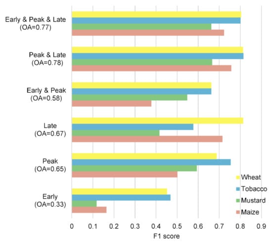
Figure 5.
F1 scores for identifying different crops using images from different periods of the 2016–2017 growing season. The values inside the parentheses on the y-axis show overall accuracies (OAs) for the given combination of images from different periods of the growing season.
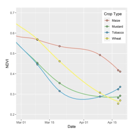
Figure 6.
Average NDVI values across all training and test pixels for each crop type for the end of the growing season.
4. Discussion
This study explored the ability of three readily available, high-resolution sensors (Planet, Sentinel-1, and Sentinel-2) to identify four major winter-season crops (wheat, mustard, tobacco, and maize) across smallholder farming systems in eastern India. We found that we were able to map crop type with high accuracies (85%), particularly when using all three sensors. Accuracies varied across crop type, with the highest accuracy for wheat and the lowest accuracy for mustard, and these patterns remained largely consistent across sensor combinations. Among the sensors considered in this study, Planet satellite data led to the greatest improvements in classification accuracy, both in single and multi-sensor models; in particular, Planet data improved the classification accuracy of the smallest farms. Finally, we found that images from the peak and late stages of the crop calendar led to the highest accuracies, and early-season imagery contributed little to the crop classification accuracy. Overall, our results suggest that crop type in smallholder systems can be accurately mapped using readily available satellite imagery, even in systems with very small field sizes (<0.05 ha) and high heterogeneities in crop type across farms.
Considering which sensor(s) lead to the highest classification accuracy, we found that the highest accuracies were achieved when using the model that included all three sensors (85%). The overall accuracy of this model was 3% higher than that of the best two-sensor model, and 13% higher than that of the best one-sensor model. This suggests that including all three sensors is important for mapping crop type. Among the two-sensor models, all sensor combinations performed similarly (80–82% overall accuracy), though the model that did not include Planet data had an accuracy that was 2% lower than those of models that included Planet data. Considering single-sensor models, we found that using only Planet data led to the highest overall accuracy (73%), though this model performed similarly to the one that used only Sentinel-2 data (72%). Sentinel-1 led to the lowest-accuracy models, despite having the best temporal coverage of all three sensors (Figure 2). This is interesting given that previous studies have shown that Sentinel-1 provides benefits for mapping crop type, particularly in regions with high cloud cover and haze [17,36].
Overall, among the three sensors used in this study, we found that Planet satellite data led to the highest accuracies when using a single sensor and to the greatest improvement in accuracies when using multiple sensors (Table 4). These results are similar to those from previous studies that found that including Planet satellite data, along with Sentinel-1 and Sentinel-2 data, improved crop type classification in smallholder systems in Africa [16,17], and that including data from other high-resolution sensors, such as RapidEye (5 m), improved small farm classification [37]. We believe improved spatial resolution was the main reason Planet models had the highest accuracy given that Planet imagery had more limited temporal and spectral resolutions compared to other sensors; Planet had the fewest scenes available throughout the growing season (Figure 2) and had fewer spectral bands and indices compared to Sentinel-2 (Table 2). The reason that the high spatial resolution of Planet satellite data (3 m) is likely important is because it better matches the spatial resolution of smallholder farms and reduces the chance of mixed pixels at field edges [15] (Figure 7).
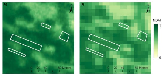
Figure 7.
Several field polygons overlaid on (A) Planet satellite imagery and (B) Sentinel-2 satellite imagery. The spatial resolution of Planet (3 m; A) better matches the size of fields and results in fewer mixed pixels compared to Sentinel-2 imagery (10 m; B).
Considering the impact of farm size on classification accuracy, we found that larger farms (600 m2) had higher classification accuracies than small farms did (600 m2, Table 6). In addition, we found that the benefit of including Planet imagery was larger considering the classification accuracy of small farms, though the improvement in accuracy was not very different between small and large farms (6% vs. 4%, respectively). We also found that the classification accuracy varied based on crop type, with the highest classification accuracies for wheat and tobacco, and the lowest classification accuracy for mustard (Table 5). One reason for the reduced classification accuracy for mustard may be that mustard fields were smallest across the four crop types considered in our study, and our results suggest that the SVM performed better for larger farms (Table 6). In addition, all crops are irrigated in this region, and previous work has shown that vegetation indices become more similar between mustard and wheat in irrigated systems [14].
The classification accuracy also varied based on the timing of imagery used (Figure 5). Early-season images did little to improve classification accuracies, likely because crops are challenging to differentiate during the early stages of crop growth when crops have little biomass [38]. Peak- and late-season imagery were found to be particularly useful for classifying crop type, with peak-season images improving the classification accuracies for mustard and tobacco and late-season images improving the classification accuracies for maize and wheat. This is likely due to differences in the planting and harvest dates of these four crops, with mustard and tobacco being harvested earlier (late March) than wheat and maize (early to late April; Figure 6). These results suggest that only using imagery for the second half of the crop growth cycle is likely adequate for mapping crop types in this area.
There were several limitations to our study. First, our study area was relatively small and it is unclear how well the results from our study may generalize to other locations across India or other smallholder systems. Nevertheless, we believe that the main findings of our study are likely applicable across systems, particularly the importance of including Planet imagery when classifying smallholder fields. Second, we conducted our study during the largely dry winter season when there is relatively little cloud cover and haze compared to the monsoon growing season. It is likely that the inclusion of Sentinel-1 would become more important during the monsoon season when there may be limited optical data available due to cloud cover and haze [39]. Future work should examine how generalizable our findings are to the monsoon season, which is the main agricultural growing season across India. Finally, we relied on an SVM classifier, which can be computationally and time-intensive to run when using a large training data set or number of features [18]. Future work should examine how well more computationally efficient classifiers, such as random forest, perform in mapping smallholder crop types.
5. Conclusions
In this study, we assessed the ability of three readily available, high-resolution sensors (Sentinel-1, Sentinel-2, and Planet) to detect four major crop types across smallholder farming systems in eastern India. We found that using all three sensors led to the highest classification accuracy (85%). Planet satellite imagery was important for classifying crop types in this system, leading to the greatest increases in classification accuracy, particularly for the smallest farms (600 m2). Furthermore, our results suggest that using only imagery from the second half of the growing season is adequate to differentiate crop types in this system. Overall, our results suggest that Sentinel-1, Sentinel-2, and PlanetScope imagery can be used to accurately map crop type, even in heterogeneous systems with small field sizes such as those in India.
Supplementary Materials
The following are available online at https://www.mdpi.com/article/10.3390/rs13101870/s1, Table S1. Confusion matrix when all three sensors were used; Table S2. Confusion matrix across small fields using Sentinel-1, and Sentinel-2 data; Table S3. Confusion matrix across small fields using Planet, Sentinel-1, and Sentinel-2 data; Table S4. Confusion matrix across large fields using Sentinel 1 and 2 data; Table S5. Confusion matrix across large fields using Planet, Sentinel-1, and Sentinel-2 data; Table S6. Confusion matrix using early season imagery from all three sensors; Table S7. Confusion matrix using peak season imagery from all three sensors; Table S8. Confusion matrix using late season imagery from all three sensors; Table S9. Confusion matrix using early and peak season imagery from all three sensors; Table S10. Confusion matrix using peak and late season imagery from all three sensors; Table S11. Confusion matrix using early, peak, and late season imagery from all three sensors.
Author Contributions
Conceptualization, M.J., B.S., A.K.S., D.B.L., and P.R.; data collection, A.K.S. and S.P.; methodology, M.J., P.R., and W.Z.; formal analysis, P.R. and W.Z.; writing—original draft preparation, P.R., M.J., and N.B.; writing—review and editing, all authors. All authors have read and agreed to the published version of the manuscript.
Funding
This research was funded by the NASA Land Cover and Land Use Change Program, grant number (NNX17AH97G), awarded to M.J.
Institutional Review Board Statement
Ethical review and approval were waived for this study, as the study was deemed to not meet the definition of human subjects research.
Data Availability Statement
Data are available from the corresponding author upon request (mehajain@umich.edu).
Acknowledgments
We would like to thank the CIMMYT-CSISA field team for collecting the data used in this study. We would also like to thank Andrew Wang for help in formatting tables.
Conflicts of Interest
The authors declare no conflict of interest.
References
- Ricciardi, V.; Ramankutty, N.; Mehrabi, Z.; Jarvis, L.; Chookolingo, B. How much of the world’s food do smallholders produce? Glob. Food Secur. 2018, 17, 64–72. [Google Scholar] [CrossRef]
- Lowder, S.K.; Skoet, J.; Raney, T. The number, size, and distribution of farms, smallholder farms, and family farms worldwide. World Dev. 2016, 87, 16–29. [Google Scholar] [CrossRef]
- Lobell, D.B.; Burke, M.B.; Tebaldi, C.; Mastrandrea, M.D.; Falcon, W.P.; Naylor, R.L. Prioritizing climate change adaptation needs for food security in 2030. Science 2008, 319, 607–610. [Google Scholar] [CrossRef] [PubMed]
- Cohn, A.S.; Newton, P.; Gil, J.D.B.; Kuhl, L.; Samberg, L.; Ricciardi, V.; Manly, J.R.; Northrop, S. Smallholder agriculture and climate change. Annu. Rev. Environ. Resour. 2017, 42, 347–375. [Google Scholar] [CrossRef]
- Jain, M.; Singh, B.; Srivastava, A.A.K.; Malik, R.K.; McDonald, A.J.; Lobell, D.B. Using satellite data to identify the causes of and potential solutions for yield gaps in India’s wheat belt. Environ. Res. Lett. 2017, 12, 094011. [Google Scholar] [CrossRef]
- Lobell, D.B. The use of satellite data for crop yield gap analysis. Field Crops Res. 2013, 143, 56–64. [Google Scholar] [CrossRef]
- Jain, M.; Mondal, P.; DeFries, R.S.; Small, C.; Galford, G.L. Mapping cropping intensity of smallholder farms: A comparison of methods using multiple sensors. Remote Sens. Environ. 2013, 134, 210–223. [Google Scholar] [CrossRef]
- Jain, M.; Singh, B.; Rao, P.; Srivastava, A.K.; Poonia, S.; Blesh, J.; Azzari, G.; McDonald, A.J.; Lobell, D.B. The impact of agricultural interventions can be doubled by using satellite data. Nat. Sustain. 2019, 2, 931–934. [Google Scholar] [CrossRef]
- Jin, Z.; Azzari, G.; You, C.; di Tommaso, S.; Aston, S.; Burke, M.; Lobell, D.B. Smallholder maize area and yield mapping at national scales with google earth engine. Remote Sens. Environ. 2019, 228, 115–128. [Google Scholar] [CrossRef]
- Jain, M.; Naeem, S.; Orlove, B.; Modi, V.; DeFries, R.S. Understanding the causes and consequences of differential decision-making in adaptation research: Adapting to a delayed monsoon onset in Gujarat, India. Glob. Environ. Change 2015, 31, 98–109. [Google Scholar] [CrossRef]
- Kurukulasuriya, P.; Mendelsohn, R. Crop switching as a strategy for adapting to climate change. Afr. J. Agric. Resour. Econ. 2008, 2, 1–22. [Google Scholar]
- Wang, S.; di Tommaso, S.; Faulkner, J.; Friedel, T.; Kennepohl, A.; Strey, R.; Lobell, D.B. Mapping crop types in Southeast India with smartphone crowdsourcing and deep learning. Remote Sens. 2020, 12, 2957. [Google Scholar] [CrossRef]
- Useya, J.; Chen, S. Exploring the potential of mapping cropping patterns on smallholder scale croplands using sentinel-1 SAR data. Chin. Geogr. Sci. 2019, 29, 626–639. [Google Scholar] [CrossRef]
- Gumma, M.K.; Tummala, K.; Dixit, S.; Collivignarelli, F.; Holecz, F.; Kolli, R.N.; Whitbread, A.M. Crop type identification and spatial mapping using sentinel-2 satellite data with focus on field-level information. Geocarto Int. 2020, 1–17. [Google Scholar] [CrossRef]
- Jain, M.; Srivastava, A.K.; Singh, B.; McDonald, A.; Malik, R.K.; Lobell, D.B. Mapping smallholder wheat yields and sowing dates using micro-satellite data. Remote Sens. 2016, 8, 860. [Google Scholar] [CrossRef]
- Rustowicz, R.M.; Cheong, R.; Wang, L.; Ermon, S.; Burke, M.; Lobell, D. Semantic segmentation of crop type in Africa: A novel dataset and analysis of deep learning methods. In Proceedings of the IEEE/CVF Conference on Computer Vision and Pattern Recognition (CVPR) Workshops, Long Beach, CA, USA, 16–20 June 2019; pp. 75–82. [Google Scholar]
- Kpienbaareh, D.; Sun, X.; Wang, J.; Luginaah, I.; Kerr, R.B.; Lupafya, E.; Dakishoni, L. Crop type and land cover mapping in northern Malawi using the integration of sentinel-1, sentinel-2, and planetscope satellite data. Remote Sens. 2021, 13, 700. [Google Scholar] [CrossRef]
- Khatami, R.; Mountrakis, G.; Stehman, S.V. A meta-analysis of remote sensing research on supervised pixel-based land-cover image classification processes: General guidelines for practitioners and future research. Remote Sens. Environ. 2016, 177, 89–100. [Google Scholar] [CrossRef]
- Gorelick, N.; Hancher, M.; Dixon, M.; Ilyushchenko, S.; Thau, D.; Moore, R. Google earth engine: Planetary-scale geospatial analysis for everyone. Remote Sens. Environ. 2017, 202, 18–27. [Google Scholar] [CrossRef]
- Wilson, R.T. Py6S: A python interface to the 6S radiative transfer model. Comput. Geosci. 2013, 51, 166–171. [Google Scholar] [CrossRef]
- Vermote, E.F.; Tanre, D.; Deuze, J.L.; Herman, M.; Morcette, J.-J. Second simulation of the satellite signal in the solar spectrum, 6S: An overview. IEEE Trans. Geosci. Remote Sens. 1997, 35, 675–686. [Google Scholar] [CrossRef]
- Fletcher, R.S. Using vegetation indices as input into random forest for soybean and weed classification. Am. J. Plant Sci. 2016, 7, 720–726. [Google Scholar] [CrossRef]
- Gurram, R.; Srinivasan, M. Detection and estimation of damage caused by thrips thrips tabaci (lind) of cotton using hyperspectral radiometer. Agrotechnology 2014, 3. [Google Scholar] [CrossRef]
- Tucker, C.J. Remote sensing of leaf water content in the near infrared. Remote Sens. Environ. 1980, 10, 23–32. [Google Scholar] [CrossRef]
- Hatfield, J.L.; Prueger, J.H. Value of using different vegetative indices to quantify agricultural crop characteristics at different growth stages under varying management practices. Remote Sens. 2010, 2, 562–578. [Google Scholar] [CrossRef]
- Filella, I.; Serrano, L.; Serra, J.; Peñuelas, J. Evaluating wheat nitrogen status with canopy reflectance indices and discriminant analysis. Crop Sci. 1995, 35. [Google Scholar] [CrossRef]
- Remote Estimation of Leaf Area Index and Green Leaf Biomass in Maize Canopies—Gitelson—2003—Geophysical Research Letters—Wiley Online Library. Available online: https://agupubs-onlinelibrary-wiley-com.proxy.lib.umich.edu/doi/full/10.1029/2002GL016450 (accessed on 4 March 2021).
- Peña-Barragán, J.M.; Ngugi, M.K.; Plant, R.E.; Six, J. Object-based crop identification using multiple vegetation indices, textural features and crop phenology. Remote Sens. Environ. 2011, 115, 1301–1316. [Google Scholar] [CrossRef]
- McNairn, H.; Protz, R. Mapping corn residue cover on agricultural fields in Oxford county, Ontario, using thematic mapper. Can. J. Remote Sens. 1993, 19, 152–159. [Google Scholar] [CrossRef]
- Vreugdenhil, M.; Wagner, W.; Bauer-Marschallinger, B.; Pfeil, I.; Teubner, I.; Rüdiger, C.; Strauss, P. Sensitivity of sentinel-1 backscatter to vegetation dynamics: An Austrian case study. Remote Sens. 2018, 10, 1396. [Google Scholar] [CrossRef]
- Planet Team. Planet Application Program Interface: In Space for Life on Earth; Planet Team: San Francisco, CA, USA, 2017; Available online: https://Api.Planet.Com (accessed on 1 March 2018).
- Houborg, R.; McCabe, M.F. A cubesat enabled spatio-temporal enhancement method (CESTEM) utilizing planet, landsat and MODIS data. Remote Sens. Environ. 2018, 209, 211–226. [Google Scholar] [CrossRef]
- Hijmans, R.J. Raster: Geographic Data Analysis and Modeling; R Package Version 3.4-5. 2020. Available online: https://CRAN.R-project.org/package=raster (accessed on 1 March 2018).
- R Core Team. R: A language and environment for statistical computing. R Foundation for Statistical Computing: Vienna, Austria, 2021. Available online: https://www.R-project.org/ (accessed on 1 March 2018).
- Kuhn, M. caret: Classification and Regression Training. R package version 6.0-86. 2020. Available online: https://CRAN.R-project.org/package=caret (accessed on 1 March 2018).
- Van Tricht, K.; Gobin, A.; Gilliams, S.; Piccard, I. Synergistic use of radar sentinel-1 and optical sentinel-2 imagery for crop mapping: A case study for Belgium. Remote Sens. 2018, 10, 1642. [Google Scholar] [CrossRef]
- Crnojevic, V.; Lugonja, P.; Brkljac, B.; Brunet, B. Classification of small agricultural fields using combined landsat-8 and rapideye imagery: Case study of Northern Serbia. J. Appl. Remote Sens. 2014, 8, 83512. [Google Scholar] [CrossRef]
- Bannari, A.; Morin, D.; Bonn, F.; Huete, A.R. A review of vegetation indices. Remote Sens. Rev. 1995, 13, 95–120. [Google Scholar] [CrossRef]
- Ferrant, S.; Selles, A.; Le Page, M.; Herrault, P.-A.; Pelletier, C.; Al-Bitar, A.; Mermoz, S.; Gascoin, S.; Bouvet, A.; Saqalli, M.; et al. Detection of irrigated crops from sentinel-1 and sentinel-2 data to estimate seasonal groundwater use in South India. Remote Sens. 2017, 9, 1119. [Google Scholar] [CrossRef]


Publisher’s Note: MDPI stays neutral with regard to jurisdictional claims in published maps and institutional affiliations. |
© 2021 by the authors. Licensee MDPI, Basel, Switzerland. This article is an open access article distributed under the terms and conditions of the Creative Commons Attribution (CC BY) license (https://creativecommons.org/licenses/by/4.0/).