Abstract
Inland open water bodies often pose a systematic error source in the passive remote sensing retrievals of soil moisture. Water temperature is a necessary variable used to compute water emissions that is required to be subtracted from satellite observation to yield actual emissions from the land portion, which in turn generates accurate soil moisture retrievals. Therefore, overestimation of soil moisture can often be corrected using concurrent water temperature data in the overall mitigation procedure. In recent years, several data sets of lake water temperature have become available, but their specifications and accuracy have rarely been investigated in the context of passive soil moisture remote sensing on a global scale. For this reason, three lake temperature products were evaluated against in-situ measurements from 2007 to 2011. The data sets include the lake surface water temperature (LSWT) from Global Observatory of Lake Responses to Environmental Change (GloboLakes), the Copernicus Global Land Operations Cryosphere and Water (C-GLOPS), as well as the lake mix-layer temperature (LMLT) from the European Centers for Medium-Range Weather Forecast (ECMWF) ERA5 Land Reanalysis. GloboLakes, C-GLOPS, and ERA5 Land have overall comparable performance with Pearson correlations (R) of 0.87, 0.92 and 0.88 in comparison with in-situ measurements. LSWT products exhibit negative median biases of −0.27 K (GloboLakes) and −0.31 K (C-GLOPS), whereas the median bias of LMLT is 1.56 K. When mapped from their respective native resolutions to a common 9 km Equal-Area Scalable Earth (EASE) Grid 2.0 projection, similar relative performance was observed. LMLT and LSWT data are closer in performance over the 9 km grid cells that exhibit a small range of lake cover fractions (0.05–0.5). Despite comparable relative performance, ERA5 Land shows great advantages in spatial coverage and temporal resolution. In summary, an integrated evaluation on data accuracy, long-term availability, global coverage, temporal resolution, and regular forward processing with modest data latency led us to conclude that LMLT from the ERA5 Land Reanalysis product represents the most optimal path for use in the development of a long-term soil moisture product.
1. Introduction
Soil moisture is a critical component of the Earth’s systems, mainly because of its capability to control surface energy fluxes, potentially exchange with the atmosphere, and partitioning precipitation into infiltration and surface runoff in terms of water budget [1,2,3,4]. Given its relatively slow variance, soil moisture has been recognized as an essential variable in climatic studies and numerical weather predictions [1,3]. Knowledge of accurate soil moisture measurements could benefit a variety of applications, ranging from drought monitoring, flood and landslide prevention, agricultural productivity improvements, and weather forecasts [1,2,3]. However, a global coverage of long-term soil moisture monitoring by in-situ measurements is impractical only from the perspectives of expenditure and manpower required by the operation and maintenance of the associated facilities.
In recent decades, satellite-based surface soil moisture products have created extensive opportunities to study terrestrial-atmosphere interactions and hydrological cycles at a global scale. Compared to optical and active microwave sensors, passive microwave sensors are more sensitive to surface soil moisture in the presence of the same confounding factors (e.g., clouds, vegetation, surface roughness, etc.) [5,6] while offering more frequent repeat global coverage of about 2–3 days, as compared to more than 10 days by active sensors. These advantages of passive microwave remote sensing of soil moisture have been the principal driving force behind the application of various spaceborne radiometers (e.g., Special Sensor Microwave Imager (SSMI) [7], Advanced Microwave Scanning Radiometer (AMSR-E) [8], Soil Moisture and Ocean Salinity (SMOS) [9] and Soil Moisture Active Passive (SMAP) [3]) for soil moisture retrieval over the last decade. Lately, there has been tremendous progress in the area of improving the spatial resolution of satellite derived soil moisture to 1 km [10,11,12] and 400 m [13].
However, the accuracy of soil moisture retrieved from satellite observations can be influenced by several factors [14], such as vegetation, topography, surface roughness etc. Inland open water bodies (e.g., lakes, rivers, wetlands, etc.) are also an important error source for passive remote sensing of soil moisture [14,15,16]. Specifically, signals detected by satellite sensors include both emissions by land areas as well as water bodies. Without proper correction procedures, the contribution of the microwave emissions of water can add to microwave emissions from adjacent land, resulting a systematic wet bias in soil moisture estimates [14]. To mitigate this contamination, it is necessary to separate the mixture of land-water brightness temperature and remove the partial emissions contributed by water bodies. This can be achieved through subtraction of water emissions from the total brightness temperatures. Water temperature representative of inland water bodies is thereby a required variable in the estimation of water radiation within the field-of-view (FOV) of the radiometer upon antenna gain pattern correction, in addition to the fractions of water cover.
Recently, a number of assimilation and reanalysis data sets that describe long-term variations of water temperatures have been released [17,18,19]. These data sets include lake surface water temperature (LSWT) from the Global Observatory of Lake Responses to Environmental Change (GloboLakes) [17] and the Copernicus Global Operations Cryosphere and Water (C-GLOPS) [19], as well as the lake mix-layer temperature (LMLT) from the European Centers for Medium-Range Weather Forecast (ECMWF) ERA5 Land Reanalysis [18,20]. These recent LSWT products have adopted the algorithms used in estimating sea surface temperature but with modifications of processing procedures and additions of lake-related parameters [21,22], thus yielding more reliable estimations of water temperature specific to inland water bodies (compared to those derived from algorithm designed for sea surface temperature). In addition, the above LSWT and LMLT data sets are expected to provide data over the open water adjacent to land, given that they are projected in regular latitude-longitude grids, which is especially helpful for the water correction in passive soil moisture retrieval algorithms. However, these water temperature data sets are supplied at vastly different spatial and temporal resolutions [17,18,19] because of diverse computational procedures and input sources.
Lake temperature data sets that incorporate long-term satellite remote sensing observations have been widely investigated, evaluated and applied [23,24,25,26,27,28,29,30,31,32,33], since LSWT is considered as an important indicator of climate change [34] and highly related to the chemical and physical process within the water bodies [28]. In order to study lake responses to climate change, validation efforts of LSWT products are generally carried out at the lake scale or at a coarse temporal resolution [23,24,25,27,28,29]. For example, [28] evaluated the LSWT derived from the Advanced Very High Resolution Radiometer (AVHRR) with in-situ measurements over 26 European Lakes where AVHRR LSWT data have absolute biases within 2 K and Pearson Correlations (R) of more than 0.9. In addition, LSWT data provided by Landsat 5 and 7 were evaluated [29] in 59 water bodies, and their mean absolute error is 1.34 K for those grids away from the land areas more than 180 m. Moreover, studies of intra- and inter-annual variability of LSWT as a response to climate change normally requires long-term LSWT data with a coarse temporal resolution [28,31]. The authors of [31] analyzed seasonal patterns of LSWT and constructed global lake thermal regions based on the LSWT data at a half-monthly time step.
However, requirements for water temperature data of inland water bodies are greatly different in the application of water correction in the derivations of soil moisture from passive remote sensing observations. Water temperature data are expected to be representative over a large but fixed spatial scale, such as the 9 km Equal-Area Scalable Earth (EASE) Grid 2.0 [35] which is a typical satellite-based Level 2 passive soil moisture retrieval setting (e.g., SMAP). Data sets with a higher temporal frequency are more optimal and conform to the instantaneous satellite observations of soil moisture given that the surface temperature variations in time can greatly impact soil moisture retrieval. Assessments and inter-comparisons of lake water temperature data sets in the frame of soil moisture are insufficient.
LMLT data of ERA5 Land represent the average temperatures for the top layer of lakes, which are different from surface skin temperatures (on the orders of micrometers and millimeters) illustrated by satellite-based LSWT products. A default depth of 25 m has been widely used in the derivation of ERA5 Land LMLT given the unavailability of water depths over most inland water bodies [18]. Therefore, systematic discrepancies between LMLT and LSWT data sets are expected as they reflect the lake thermal conditions at different depths, but this is rarely investigated. Research from [20] updated the depth information and compared LMLT data with in-situ measurements (with only one station having hourly data), and concluded that the mean absolute errors of ERA5 Land are from 2.25 to 3.22 K. Nevertheless, the representative depth (about 1 m) of in-situ observed temperature is also different from GloboLakes and C-GLOPS LSWT products. Moreover, inter-comparisons between areal LSWT and LMLT data sets could also be useful to more or less indicate their quality over a wider geographical coverage.
In light of these, three lake temperature data sets were selected for evaluation and inter-comparison over a five-year period from 2007 to 2011, including LSWT from GloboLakes and C-GLOPS, and LMLT from ERA5 Land. Since the assessments of the above products emphasize their usefulness in providing correction for microwave emissions from open water for passive soil moisture retrieval, performance evaluation was conducted at their native spatial scales and on the 9 km EASE Grid as an illustration. The latter was used to demonstrate how these data sets perform in a larger spatial extent common in passive soil moisture retrieval products. In addition to data accuracy, several aspects were also examined in this study, which are long-term availability, global coverage, temporal resolution, regularity in data maintenance and extension.
This paper is structured as follows. Section 2 introduces the three lake temperature products and the in-situ measurements considered in this analysis. Section 3 presents the statistical metrics to quantify product performance. The evaluation results and discussions are reported in Section 4 and Section 5, respectively, followed by a summary in Section 6.
2. Study Regions and Lake Temperature Data Sets
2.1. Study Regions
In this study, the buoys used to represent the in-situ measurements of lake water temperature are distributed over 11 lakes in the North America as shown in Figure 1. Most available stations are concentrated on the Great Lakes region composed of Lake Superior (47.7°N, 87.5°W), Lake Huron (44.8°N, 82.4°W), Lake Erie (42.2°N, 81.2°W), Lake Michigan (44.0°N, 87.0 W), and Lake Ontario (43.7°N, 77.9°W). Along the border of the United States and Canada, the total surface area of these five lakes is around 244,106 km2 [36]. Additionally, the Great Lakes have abundant freshwater resources, approximately 21% of the global surface freshwater volume [37]. There are also several stations within the Great Lakes area, including Lake Saint Clair (42.5°N, 82.7°W), Lake Nipissing (46.3°N, 79.8°W), and Lake Smicoe (44.4°N, 79.3°W). The remaining three lakes are Lake Great Slave (61.5°N, 114.0°W), Lake Winnipeg (52.1°N, 97.3°W), and Lake of the Woods (49.2°N, 94.8°W) that locate in the further north regions. According to the classification of lake thermal regions developed by [31], these lakes could be grouped into Northern Temperate and Northern Cool with average temperatures around 282.95 K and 279.25 K, respectively.
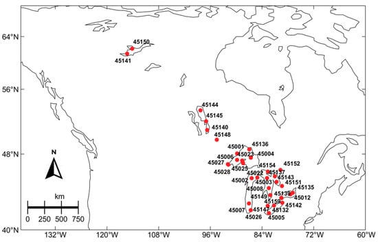
Figure 1.
Distribution of in-situ buoys (red points).
2.2. Lake Temperature Data Sets
Three lake temperature products consisting of two satellite-based LSWT and one-model based LMLT were examined in this study. The specifications of these data sets are summarized in Table 1. In-situ measurements from buoys available within the studying period were used as the reference in the validation.

Table 1.
Summary of lake temperature data sets used in this study.
2.2.1. Global Observatory of Lake Responses to Environmental Change (GloboLakes)
GloboLakes LSWT version 4.0 provides daily averages of surface water temperature for around 1000 lakes mostly extracted from the Global Lakes and Wetland Database (GLWD) Level 1 product [17,38]. The retrievals of LSWT were derived using the same algorithms on satellite observations from various types of sensors and platforms, including the Along Track Scanning Radiometer (ATSR-2) on European Remote Sensing Satellite (ERS-2), Advanced Along Track Scanning Radiometer (AATSR) on Envisat, and AVHRR on MetOpA [39]. This data set contains a long-term daily LSWT data ranging from 1995 to 2016 with a spatial resolution of 0.05°.
In this study, daily files with a regular latitude-longitude grid were used. In addition to skin temperature of lakes’ surface, the information of uncertainty estimations and quality level related to LSWT retrievals is also included in the data set. Quality level is considered as a flag to quantify the confidence of LSWT retrievals, such as the degree of interference caused by cloud contamination, and is unable to necessarily represent the accuracy level. Data with all quality levels were retained in order to satisfy the need of high temporal frequency in water correction of soil moisture retrievals. It should be noted that a static land-water mask based on the European Space Agency Climate Change Initiative (ESA CCI) Land Cover map with a spatial resolution of 300 m for the time period 2005–2010 has been applied to identify and delineate the lake pixels, which could lead to inappropriate estimations of LSWT over water bodies with dynamic surface extensions [39]. In addition, the combined use of observations from different satellite sensors will inevitably introduce more error sources despite the increase of available samples and the harmonized processing.
2.2.2. Copernicus Global Land Operations (C-GLOPS)
LSWT of C-GLOPS contains gridded 10-day mean surface water temperature over more than 1000 lakes composed of the world’s largest and those water bodies of particularly scientific interest [19]. Specifically, the 10-day LSWT data of C-GLOPS are temporally aggregated and generated via calculating the weighted average of Level 3 gridded daytime files partitioned by the 1st to 10th, and 11th to 20th, and 21st to the end of each month. Three types of LSWT are included in this data set, which are historical (v1.0.2), reprocessed (v1.0.2), and near real-time products (v1.0.1 and v1.1.0), depending on the timeliness and completeness of the Level 1b inputs during processing [26]. Since the LSWT retrievals at a regular 1/120° resolution grid are originally derived from the visible and infrared from the AATSR and Sea and Land Surface Temperature Radiometer (SLSTR) onboard Envisat, and Sentinel 3A and 3B, the temporal coverage of this data set was separated into two periods: May 2002 to April 2012, and November 2016 to present. This data set can be freely accessed and downloaded through the Copernicus Global Land Portal (https://land.copernicus.eu/global/products/lswt, accessed on 9 March 2021). Similar to GloboLakes LSWT, the uncertainty information and quality levels are also available and all quality-level data were adopted in this work.
According to [26], the accuracy of C-GLOPS overall fulfills the uncertainty requirement of 1 K comparing against in-situ measurements. However, the utilization of LSWT with a quality level lower than 3 should be handled carefully [22]. Again, one common factor that could influence the observations is the presence of clouds given that the AATSR and SLSTR operate at visible and infrared bands [22]. Additionally, the application of a uniform threshold standard has risks in the identification of water and non-water grid cells [22]. Contamination from land associated signals could affect the retrieval quality. As a result, LSWT retrievals in the areas near the land are more likely to have lower performance. Moreover, the numbers and observation times used in the temporal aggregation varies from place to place, possibly leading to spatially or temporally inconsistent thermal conditions, even for the same lake [22]. Furthermore, a static mask representing the maximum surface water extent of lakes from 2015 to 2010 was adopted [22], which is improper for those water bodies with evident changes in areas at the 1 km2 scale.
2.2.3. ERA5 Land
ERA5 Land is a reanalysis product containing a series of variables that describe the state of various land components from 1981 to the current time [18,20]. Although ERA5 Land utilizes ERA5 atmospheric forcing as inputs to derive the land components, the ERA5 Land data set has a higher spatial resolution at 0.1° compared to its predecessor at 0.25°. Without coupling with the atmospheric module of ECMWF’s Integrated Forecasting System and ocean wave models as well as data assimilation, the processes related to the computation and delivery of ERA5 Land are expected to be more efficient. The core of ERA5 Land is the Tiled ECMWF Scheme for Surface Exchanges over Land incorporating land surface hydrology (H-TESSEL) (version CY45R1) [40].
In this study, hourly LMLT from the ERA5 Land data set was selected to reflect the thermal conditions over various inland water bodies. The ECMWF Integrated Forecasting System separates the vertical structure of inland water bodies into two levels: the upper (mix layer) and lower (thermocline layer) layers given the implementation of the Flake model [41,42]. In light of this, LMLT represents the average water temperature at the uppermost layer of lakes and differs from skin temperature at the water surface. Lake-related variables can be calculated for each pixel so as to incorporate the sub-grid features of the small to medium-size lakes [20,42,43]. ERA5 Land data set provides a spatially complete temperature map for both inland water bodies and coastal waters, but it is necessary to use an auxiliary data set that describes the water fraction within the grid cell simultaneously with LMLT. This static map of lake cover is provided by the reanalysis product of ERA5 (https://cds.climate.copernicus.eu/cdsapp#!/dataset/reanalysis-era5-single-levels?tab=overview, accessed on 15 November 2020) at 0.25° and then interpolated into 0.1° and the 9 km EASE grid. For inland water bodies where lake depths are not available, a default value of 25 m has been used [18], which is likely to result in unreasonable LMLT retrievals, especially for those lakes with shallow depths.
2.2.4. In-Situ Measurements of Lake Surface Temperature
In-situ lake surface temperatures collected by the moored buoys from fixed locations were used to benchmark the performance of assimilated and reanalysis products. Based on the stations considered in the Quality Validation Report of C-GLOPS [26], 34 buoys (Table A1 in Appendix A) over lakes in Northern America were selected. These measurements are from either the National Data Buoy Center (NDBC) (https://www.ndbc.noaa.gov/, accessed on 14 March 2021) or Fisheries and Ocean Canada (FOC) (https://www.meds-sdmm.dfo-mpo.gc.ca/isdm-gdsi/waves-vagues/data-donnees/index-eng.asp, accessed on 14 March 2021). Figure 1 describes the geographical locations of in-situ measurements. Historical files of hourly water temperature can be used in validation for remotely-sensed and modelled lake temperature data sets.
3. Methodology and Assessment Metrics
3.1. Validation against In-Situ Measurements
Evaluation of lake temperature data sets were firstly assessed by comparing against 34 in-situ buoys distributed in the North America at their native spatial and temporal resolutions. LSWT data of all quality levels from GloboLakes and C-GLOPS were retained in the assessments to incorporate as many observations as possible. Although low-quality-level samples does not necessarily represent inferior accuracy, the overall better statistic metrics for LSWT data at quality levels of 4 or 5 have been obtained [26]. Despite that, the degradation on the performance of LSWT data sets is expected to be limited as the majority of LSWT data with quality levels of 4 and 5 [26]. Following a similar manner used in [15], data with water temperature below 275.15 K (2 °C) were screened out to avoid unreliable observations near the freezing point.
Given that in-situ data were collected from different sources (Table A1), quality control measures have been adopted to filter out those abnormal and suspicious observations. A pre-determined threshold (in addition to 275.15 K mentioned above) and manual inspection were used. Firstly, a threshold of 306.55 K was employed and those in-situ observations with temperatures above this value were removed. This boundary value represents the maximum temperature for lakes under Northern Temperate and Northern Cool classifications (all in-situ stations are within these areas) [31]. Then, some sudden spikes or extremely low temperatures described by the in-situ time series were manually masked.
Since the temporal resolutions of in-situ observation, LMLT and LSWT data sets vary from sub-hourly to 10-day intervals, temporal averaging procedures were required before assessments. Similar to the steps applied in [26], for example, 10-day averages of in-situ observations were computed for evaluating C-GLOPS LSWT. In addition, it should be noted that data from in-situ observations, ERA5 Land, GloboLakes, and C-GLOPS reflect water temperature at different depths. Generally, LSWT data measured by satellite instruments could represent the water temperature from many micrometers to a few millimeters depending on the instrument frequencies, whereas the in-situ buoys usually detect the water temperature at around 1 meter (as described in Table A1) under the water surface and without significant effects from diurnal cycles. In terms of ERA5 Land, LMLT reflects the average temperature for the top-most layers of lakes and its corresponding depth is dependent on lake depth used in the Flake model [20]. However, a default depth of 25 meters was used in the derivations of LMLT over most inland water bodies due to the common unavailability of depth information [18]. Therefore, discrepancies between LMLT and LSWT are expected to exist but have not been widely investigated yet. Regarding the LSWT and in-situ observations, skin effect could account for the -0.2 K error mainly generated by the different observing depths between in-situ measurements and satellite sensors [26]. The remaining residuals could be contributed by other unquantified factors, such as the near-surface stratification, underestimating atmospheric attenuation or overestimating surface emissivity [26,27].
Subsequently, ERA5 Land, GloboLakes, and C-GLOPS were resampled into the EASE 9 km scale by bilinear interpolation in order to quantify the performances of these data sets in the context of soil moisture retrievals as well as analyze the influences on their data accuracy by rescaling processing. Again, in-situ measurements were used as reference to assess the performances of three lake temperature products at the 9 km EASE grid after temporal averaging. It should be noted that statistical metrics were considered to be effective and calculated only if there are at least 30 paired data between two data sets [44,45,46]. In addition to the uncertainty of products, seasonal trends captured by lake temperature data sets were also illustrated and examined by time series over Lake Superior and Lake Huron. Furthermore, dependency of errors between the above data sets and in-situ measurements on temperature ranges were also investigated.
3.2. Inter-Comparisons among Lake Temperature Products at the 9 km Scale
Due to the fact that in-situ measurements are only available in the limited geographical regions, a global-scale assessment based on in-situ observations is difficult to achieve. Therefore, inter-comparisons among different lake temperature products could be an effective alternative to corroborate their relative performances. It is particularly feasible when the LSWT retrieval algorithm is found on physics [26] to guarantee the consistency of derived LSWT values. The EASE 9 km grid cells with lake fractions smaller than 0.05 were not considered in accordance the requirements of passive remote sensing soil moisture retrieval algorithm.
Following similar steps adopted in the Section 3.1, overlapped pixels among three lake temperature data sets were firstly determined and then temporal averaging was separately applied before three groups of pairwise comparisons (Figure 2). For example, EAR5 Land hourly LMLT data were temporally aggregated at a 10-day scale prior to comparing with C-GLOPS LSWT. The general workflow adopted for the assessments and comparisons of performances of considered water temperature data sets has been described in Figure 2, and different filling colors correspond to various temporal scales. Additionally, differences and correlations among LMLT and LSWT products were studied conditioned by lake cover fractions. More importantly, the numbers of available pixels and data during the studying period were investigated and compared given that the requirements of high temporal resolution and wide spatial coverage in the soil moisture retrievals.
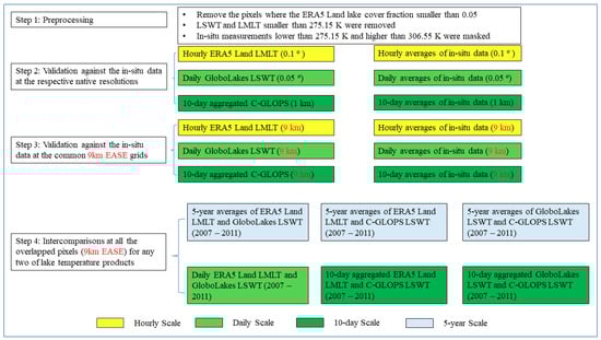
Figure 2.
Schematic diagram that describes the work flow adopted in this study for evaluating the performance of lake temperature data sets. Different colors of the boxes indicate different temporal scales of data sets.
3.3. Assessment Metrics
Six statistical metrics were adopted to reflect the accuracy of assessed products, which are mean bias, standard deviations of bias, root mean square error (RMSE), the Pearson correlation coefficient (R), median bias, and robust standard deviation (RSD). Standard deviation and RSD describe the dispersion of mean bias and median bias, respectively. Robust statistical metrics (i.e., median bias and RSD) were considered because they are less susceptible to outliers due to extreme observations [26]. However, unreliable estimations of water temperature over inland water bodies are inevitable, possibly due to the undetected clouds or horizontal variability at water surface caused by winds [21,26]. RSD is calculated as the following steps: (1) calculate the absolute differences between the biases and median bias (2) determine the median value of those prior absolute differences (3) multiply a factor (1.5) with the median value obtained in Step (2) as RSD [26]. Here, water temperatures from the evaluated data sets and in-situ measurements are denoted as and . The formulas of those statistical metrics are given in Equations (1)–(6), where , , , , and represent the arithmetic mean, median, standard deviation, mean bias, and the number of samples, respectively.
4. Results
In this section, assessment results of LMLT from ERA5 Land and LSWT from GloboLakes and C-GLOPS are presented. Firstly, validations against their corresponding temporal averaged in-situ measurements were conducted to reflect their innate performances at native scales. Time series and scatter plots were applied to describe the consistency in terms of the seasonal trends and proximity of absolute values among different products. In the framework of passive remote sensing soil moisture retrievals, the performances of ERA5 Land, GloboLakes and C-GLOPS at the EASE 9 km pixels were further analyzed, and the effects of the errors along the increased temperatures were also investigated. Additionally, spatial coverages, temporal resolutions, and overlapped pixels of LMLT and LSWT data sets were studied and prepared for inter-comparisons over wider areas where in-situ measurements are scarce or unavailable. Discrepancies between LMLT and LSWT products were then examined across various lake cover fractions.
4.1. Overall Performance of Lake Temperature Products at Their Original Resolutions
Figure 3 describes the boxplots of median bias, RMSE and R for hourly LMLT of ERA5 Land, daily LSWT of GloboLakes, and 10-day aggregated LSWT from C-GLOPS, relative to the lake temperature from in-situ observations. In terms of median bias and RMSE, LSWT from GloboLakes and C-GLOPS is closer to in-situ measurements than LMLT from ERA5 Land. LSWT products tend to underestimate while ERA5 Land product is inclined to overestimate. Additionally, all three data sets have exhibited a strong capacity to capture the temporal variations because their R values are consistently higher than 0.8. In general, marginally inferior accuracy of ERA5 Land is expected because LSWT data from GloboLakes and C-GLOPS are able to reflect the thermal conditions over smaller areas by mapping at finer spatial resolutions and thereby correspond better to point in-situ measurements.
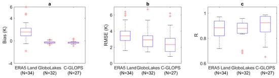
Figure 3.
Boxplots of median bias (a), RMSE (b), and R (c) for hourly LMLT of ERA5 Land, daily LSWT of GloboLakes, and 10-day LSWT of C-GLOPS at their native spatial resolutions. N represents the number of in-situ stations used to calculate the metrics.
As mentioned in Section 3, median bias and RSD are considered to be more reliable in the assessments of water temperature data sets by reducing the impacts of possibly contaminated observations, compared to mean bias and its standard deviation [26]. According to Table 2, differences between the conventional and robust statistical metrics are straightforward. RSD values of LSWT products are around half of their standard deviations whereas the discrepancies of two types of metrics are minor for LMLT from model-based ERA5 Land data set.
Table 2.
Statistical metrics between in-situ measurements and lake temperature products at their native resolutions and the 9 km EASE grid.
Comparisons of time series have been carried out over Lake Superior and Lake Huron, where several buoys are available during the studying period to further assess the seasonal consistency between in-situ measurements and lake temperature data sets. As shown in Figure 4 and Figure 5, seasonal trends of lake water temperature are relatively stable, and the maximum and minimum water temperatures occur in late summer (August or September [23]) and spring (April or May) regardless of ice cover periods. Overall, seasonal patterns and averages of lake water temperatures in Lake Superior and Lake Huron are highly similar. The ERA5 Land product has shown noticeable overestimation, especially during summer seasons compared to GloboLakes and C-GLOPS.
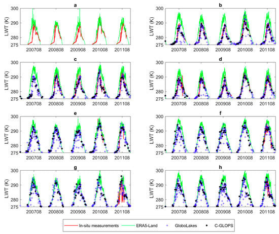
Figure 4.
Variations of lake water temperature on Lake Superior from 2007 to 2011 ((a): Station 45001 48.06°N, 89.79°W; (b): Station 45004 47.59°N, 86.59°W; (c): Station 45006 47.34°N, 89.79°W; (d): Station 45136 48.54°N, 86.95°W; (e): Station 45023 47.27°N, 88.61°W; (f): Station 45025 46.97°N, 88.40°W; (g): Station 45027 46.86°N, 91.93°W; (h): Station 45028 46.81°N, 91.83°W).
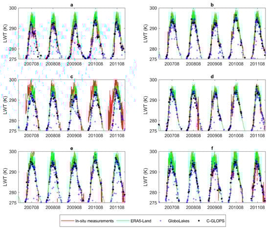
Figure 5.
Variations of lake water temperature on Lake Huron from 2007 to 2011 ((a): Station 45003 45.53°N, 82.84°W; (b): Station 45008 44.28°N, 82.42°W; (c): Station 45137 45.54°N 81.02°W; (d): Station 45143 44.94°N, 80.63°W; (e): Station 45149 43.54°N, 82.08°W; (f): Station 45154 46.05°N, 82.64°W).
According to Figure 6a–c, most data from lake temperature data sets and in-situ measurements are consistent and distributed along the 1:1 line. Again, ERA5 Land tends to overestimate, and LSWT values from GloboLakes and C-GLOPS have smaller biases relative to in-situ measurements. Over the locations where in-situ stations are considered in this study, lake water temperature data are mostly concentrated on the interval from 290 to 295 K. Deviation extents between in-situ observations and lake temperature data sets are relatively stable with the increase of water temperature (Figure 7a–c). Moreover, the ranges of differences seem to become larger under warmer conditions.
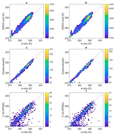
Figure 6.
Scatter plots of data from lake temperature data sets at their original resolutions (a,c,e) and at the 9 km EASE grid (b,d,f) compared to in-situ measurements. The number on the color bar represents the number of available data samples within each assigned temperature interval. Points closer to yellow mean more samples lie in that temperature range whereas these closer to blue mean less samples lie in that temperature range.
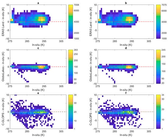
Figure 7.
Variations of errors between lake temperature data sets and in-situ measurements with the increase of water temperature at their original resolutions (a,c,e) and at the 9 km EASE grid (b,d,f). The number on the color bar represents the number of available data samples within each assigned temperature interval. Points closer to yellow mean more samples lie in that temperature range whereas these closer to blue mean less samples lie in that temperature range.
4.2. Overall Performance of Lake Temperature Products at the 9 km EASE Resolution
Lake temperature data sets were resampled to the 9 km EASE resolution and compared with in-situ measurements to measure the effects of changing spatial resolution on the estimations of lake temperature. Similar to the results obtained at their original resolutions, LSWT values from the GloboLakes and C-GLOPS have smaller bias and RMSE than LMLT from ERA5 Land (Figure 8). In terms of temporal correlations, all three data sets have comparable performances with R values of 0.89, 0.88, and 0.94 (Figure 8 and Table 2).
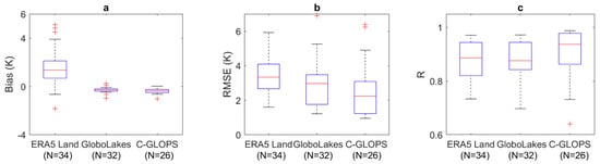
Figure 8.
Boxplots of median bias (a), RMSE (b), and R (c) for hourly LMLT of ERA5 Land, daily LSWT of GloboLakes, and 10-day LSWT of C-GLOPS at the 9 km EASE grid. N represents the number of in-situ stations used to calculate the metrics.
According to Table 2, the median bias (mean bias) of ERA5 Land, GloboLakes, and C-GLOPS are 1.36 K (1.40 K), −0.29 K (−0.90 K), and −0.36 K (−0.69 K). RSD values of LSWT products are smaller than the standard deviations of mean bias. Lake water temperatures provided by the resampled products were matched and compared with in-situ measurements at various corresponding temporal resolutions (Figure 6b,d,f). LSWT data of GloboLakes and C-GLOPS at the 9 km EASE resolution still have a good agreement with in-situ observations but the numbers of paired samples decrease compared to those at their native resolutions. As shown in Figure 7d,f, the errors between LSWT products at the coarser resolution and in-situ measurements are negatively extended.
4.3. Matchup Intercomparison of Lake Temperature Products
Comparisons of resampled lake temperature data sets have been performed on all their overlapping regions across the world to comprehensively assess the performance of ERA5 Land LMLT, GloboLakes LSWT, and C-GLOPS LSWT. Since all three lake temperature products gridded on the 9 km EASE map still have different temporal resolutions, temporal averaging is required before their inter-comparisons. As mentioned earlier, a lake cover fraction threshold of 0.05 was used to screen out some land grids. On one hand, this percentage of lake cover conforms to the threshold of static water fraction considered in SMAP in which the quality of soil moisture retrieved in areas with a water fraction of more than 5% may be unreliable [14]. On the other hand, compared to 0.5, a smaller threshold is conducive to involving as many inland water bodies as possible, especially for narrow bodies and minor water areas. The inclusion of such water bodies is essential and critical in soil moisture retrievals because small-scale shallower lakes commonly have more distinct diurnal variations in temperature than sea water or deeper lakes [42].
The number of grids with ERA5 Land product exceeds, by an order of magnitude, the GloboLakes and C-GLOPS products, which have 12781 and 11722 available pixels, respectively (Table 3). Although the temporal resolutions of GloboLakes and C-GLOPS are nominally daily and 10 days, they actually have effective LSWT data around every 4 days and 26 days, respectively. However, the ERA5 Land product has the ability to continuously update LMLT as long as the input data are available. There are a total of 10,111 grids where all three products have available temperature data that are necessarily obtained in coincidence. It should be noted that there may be only one effective LSWT in certain overlapped grids. Those pixels are distributed over various locations spanning from the Arctic region to Africa. Long-term frozen conditions could be one possible reason leading to very few observations for high-latitude grids.
Table 3.
Spatial and temporal characteristics of lake temperature data sets.
Based on the available overlapping pixels between any two lake temperature products, 5-year averages were calculated to represent the grid-scale water temperatures. According to Figure 9, lake water temperatures from all three products are close to each. 5-year averages of LMLT are overall higher than 5-year averages of LSWT, with the results comparing consistently against the in-situ measurements. At the range from 280 to 285 K, 5-year averages of LSWT from C-GLOPS are slightly higher than those from GloboLakes, partially due to a small number of C-GLOPS LSWT samples over some pixels.
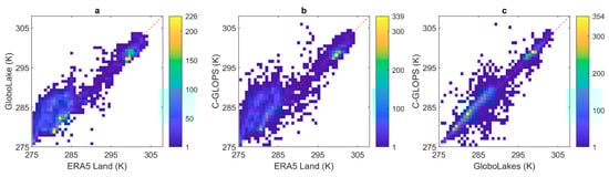
Figure 9.
Scatter plots of 5-year averages lake temperature data. (a): GloboLakes versus ERA5 Land (N = 10111); (b). C-GLOPS versus ERA5 Land (N = 10111); (c). GloboLakes versus C-GLOPS (N = 10111). N represents the number of pixels with paired data. The number on the color bar represents the number of available data samples within each assigned temperature interval. Points closer to yellow mean more samples lie in that temperature range whereas these closer to blue mean less samples lie in that temperature range.
As shown in Figure 10, those statistical metrics were computed based on Figure 10a,d: daily ERA5 Land LMLT and daily GloboLakes LSWT, Figure 10b,e: 10-day ERA5 Land LMLT and 10-day C-GLOPS, and Figure 10c,f: 10-day GloboLakes LSWT and 10-day C-GLOPS. In addition, their discrepancies were further conditioned by the lake cover fractions. Again, the composite 10-day LSWT from GloboLakes and C-GLOPS have shown great consistency in both absolute values and temporal variations because of the utilization of observations from AATSR (Figure 10c,f). In addition, ERA5 Land products have also exhibited high correlations with GloboLakes and C-GLOPS on R values near or even more than 0.9 (Figure 10d,e). LMLT tend to be lower than LSWT in the regions with low water coverage (0.05–0.25) whereas the scenarios are opposite over areas with more water bodies (Figure 10a,b). In terms of differences and R, data of ERA5 Land are closer to LSWT products when the lake cover fraction ranges from 0.05 to 0.5.
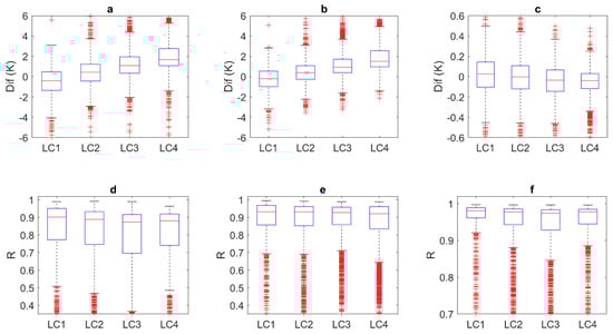
Figure 10.
Boxplots of differences and R between lake temperature data sets at the 9 km EASE grid conditioned by lake cover (LC) fractions. ‘Dif’ denotes differences between two lake temperature data sets. (a): Dif = daily ERA5 Land LMLT–daily GloboLakes LSWT (N = 9925); (b): Dif = 10-day ERA5 Land LMLT–10-day C-GLOPS LSWT (N = 9044); (c): Dif = 10-day GloboLakes LSWT–10-day C-GLOPS LSWT (N = 8969); (d): daily ERA5 Land LMLT versus daily GloboLakes LSWT; (e): 10-day ERA5 Land LMLT versus 10-day C-GLOPS LSWT; (f): 10-day GloboLakes LSWT versus 10-day C-GLOPS LSWT. The intervals of lake cover percentage represented by LC1 (0.05–0.25), LC2 (0.25–0.5), LC3 (0.5–0.75), and LC4 (0.75–1). N represents the number of pixels in which paired data from two different data sets are more than 30.
5. Discussion
The impacts of varying spatial resolutions on the performances of LSWT and LMLT products can be studied by comparisons of their statistical metrics at their original resolutions and the 9 km EASE grids. Generally, metric values at the coarser resolution are within the same magnitude and comparable to those at their original spatial resolutions. Therefore, it is expected that any given resampling procedure only has limited effects on degrading quality of lake temperature data sets, especially for ERA5 Land whose native resolution is close to the 9 km EASE grid. Despite that, absolute values of median bias of C-GLOPS and GloboLakes at the 9 km EASE grid have slightly increased. This is partly because the resampled LSWT products have a coarser resolution, representing the LSWT over broader water areas, and become more deviated from in-situ data collected at a point scale.
Underestimations of LSWT products compared to the in-situ measurements conform to previous validation results [26,27,28,29,32]. According to [26], the differences between C-GLOPS with a quality level higher than 3 and in-situ measurements are −0.24 K ± 0.88 K, which is comparable to the results shown in Table 2 (−0.31 K ± 0.93 K). A slightly larger bias could be partially caused by the consideration of all quality-level data here. In addition, all the lakes with positive biases presented in [26] are not included in this study, possibly leading to a higher negative median bias. A negative 0.2 K error between the LSWT and in-situ data is considered to be normal due to the cool skin effect of surface water temperature relative to in-situ measurements of the sub-surface [26]. Similarly, systematic discrepancies among LMLT and LSWT products cannot be ignored since the water depths modeled by ERA5 Land (default 25 m [18]), and LSWT products (skin temperature) are different. Moreover, the mean absolute error of the ERA5 Land data set (0.1°) here is 2.83 K, close to the results shown in [20] (2.25 to 3.22 K).
Despite LSWT being closer to in-situ observations in terms of absolute values, the spatial coverage of ERA5 Land is greater than the LSWT products mainly focusing on larger water bodies [17,19] given the differences in the available pixel numbers. Additionally, as observed in Figure 4 and Figure 5, the provision of discrete or even sporadic satellite observations from GloboLakes and C-GLOPS could be insufficient to continuously reflect instantaneous thermal variations of inland water bodies required in the frame of soil moisture. As mentioned earlier, the quality of LMLT is less disturbed by the resampling procedures as well as the local weather conditions at a certain time. Moreover, ERA5 Land LMLT data are available from 1981 to present, compared to GloboLakes (1995–2016) or C-GLOPS with a gap period. Furthermore, consistently high temporal correlations of hourly LMLT and hourly in-situ measurements, daily LMLT and daily LSWT of GloboLakes, and 10-day LMLT and 10-day LSWT of C-GLOPS provide confidence in making LMLT closer to in-situ measurements by adopting proper rescaling approaches in the future. In light of these, ERA5 Land LMLT could be the optimal water temperature product used for water correction in soil moisture retrievals.
It should be noted that there are several limitations to this study. Firstly, the obtained evaluation results are based on lake temperature products from 2007 to 2011, which is only a partial portion of the temporal extent for each data set. In particular, the C-GLOPS product is separated into two intervals using observations from different satellite sensors. There might be a slight underestimation related to the quality of the C-GLOPS product, given that the newly reprocessed C-GLOPS LSWT is aggregated using the observations from SLSTR instruments with a higher temporal frequency [26].
In addition, in-situ measurements considered here are all distributed in North America and thus unable to fully represent lake temperatures globally across various climatic and geophysical conditions. However, those areas with in-situ measurements pertain to Northern Cool in terms of lake thermal regions, representing more than 40% of total lake areas [31]. The evaluation results are thereby sufficient to indicate some aspects of the quality of considered LMLT and LSWT products. The retrieval method of LSWT products is based on physics and their stable performances are expected [22], and therefore the analyses of inter-comparison results between LMLT and LSWT data sets are of more importance. Nevertheless, it is still challenging to assess those grids with inland water bodies beyond the scopes of GloboLakes and C-GLOPS. Furthermore, some areas contiguous to oceans have been excluded from the ERA5 Land data set. However, those pixels are also critical in the retrieval of global soil moisture. Therefore, plenty of products associated with sea surface temperature may be evaluated and compared with ERA5 Land LMLT in order to complement those coastal grids in future studies.
6. Conclusions
The accuracy of land surface emissions governs the quality of retrieved soil moisture products, and reasonable partitioning of water and land emissions from satellite-based observations requires accurate estimations of water temperature. In light of this, three newly released lake temperature products, ERA5 Land, GloboLakes, and C-GLOPS, have been evaluated by comparing with in-situ observations as well as inter-comparisons among them from 2007 to 2011. Six statistical metrics have been selected to reflect the performance in aspects of temporal correlations and the proximity of absolute values. Overall, the LMLT of the ECMWF ERA5 Land product has been considered as the optimal option to be used in correction procedures of passive remote sensing soil moisture retrievals due to its wide spatial coverage, long-term consistent performance, less interference from resampling procedures, and the continuous provision of hourly updated data.
Generally, the three lake temperature data sets have comparable performances and adequate capacity to capture the dynamic variations of water temperatures (indicated by R values more than 0.8). The yielded differences between lake temperature products and in-situ measurements are 1.56 K ± 2.76 K, −0.27 K ± 0.86 K, and −0.31 K ± 0.93 K in the original spatial resolutions, and 1.36 K ± 2.68 K, −0.29 K ± 0.83 K, and −0.36 ± 0.92 K in the EASE 9-km scale for ERA5 Land, GloboLakes, and C-GLOPS, respectively. In light of these, the transfer of spatial resolution from their native scales to the 9-km EASE grids has not largely affected the assessment results. Moreover, the effects of temperatures on biases between lake temperature data sets and in-situ measurements are limited. Furthermore, median bias and RSD could be more appropriate to represent the quality of lake temperature products compared to the conventional metrics.
Evidently, the ERA5 Land product has advantages in both spatial coverage and temporal resolution for satisfying the requirements for soil moisture retrievals in which lake water temperatures (for example) at 6 a.m. and 6 p.m. are needed (to coincide with the SMAP overpassing time). In terms of 5-year averages over the studying period, LMLT values are overall higher than LSWT data while the estimations of LSWT of GloboLakes and C-GLOPS are closer to each other, partially because of the utilization of observations from the same satellite sensor. Furthermore, the temporal variations of LMLT and LSWT products are highly correlated while their absolute values are closer over pixels with small water fractions in a range of 0.05 to 0.5.
Although different water depths are considered in LMLT and LSWT products as well as in-situ measurements, they exhibit similar patterns in illustrating the seasonal patterns and close values within 1.6 K to demonstrate the consistency of various considered data sets. Given those, the extensive spatial coverage, hourly updated lake temperature, and long-term availability, ERA5 Land based on the ECMWF H-TESSEL model is expected to be the best candidate for water correction in soil moisture retrievals. Additionally, this study could provide useful information related to lake temperature products for data users who are interested in the investigations of the thermal conditions of inland water bodies in the context of climate change.
Author Contributions
Conceptualization, S.C., R.B. and V.L.; methodology, R.Z., S.C., R.B. and V.L.; data analysis, R.Z. and S.C.; writing—original draft preparation, R.Z.; writing—review and editing, S.C., R.B. and V.L. All authors have read and agreed to the published version of the manuscript.
Funding
This investigation is funded as a university subcontract under the NASA Making Earth System Data Records for USE in Research Environments (MEaSUREs) Program.
Data Availability Statement
Publicly available datasets were analyzed in this study. ERA5 Land data were downloaded from Copernicus Climate Change Service (https://cds.climate.copernicus.eu/cdsapp#!/dataset/reanalysis-era5-land?tab=form, accessed on 15 November 2020). GloboLakes and C-GLOPS data are freely available on Comprehensive Environmental Data Archive (CEDA) (https://catalogue.ceda.ac.uk/uuid/76a29c5b55204b66a40308fc2ba9cdb3, accessed on 9 March 2021) and Copernicus Global Land Service (https://land.copernicus.eu/global/products/lswt, accessed on 9 March 2021). In-situ water temperature measurements are available on National Data Buoy Center (NDBC) (https://www.ndbc.noaa.gov/, accessed on 14 March 2021) and Fisheries and Ocean Canada (FOC) (https://www.meds-sdmm.dfo-mpo.gc.ca/isdm-gdsi/waves-vagues/data-donnees/index-eng.asp, accessed on 14 March 2021), respectively.
Acknowledgments
We are grateful to all contributors to the data sets used in this study.
Conflicts of Interest
The authors declare no conflict of interest.
Appendix A
Table A1.
Summary of in-situ measurements used in this study.
Table A1.
Summary of in-situ measurements used in this study.
| Index | Name/Country | Latitude | Longitude | Start Year | Buoy | Senor Depth (Meter Below Water Line) | Organization * |
|---|---|---|---|---|---|---|---|
| 1 | Superior/Canada-USA | 48.06 | −89.79 | 1979 | 45001 | 1.1 | NDBC |
| 2 | Superior/Canada-USA | 47.59 | −86.59 | 1980 | 45004 | 1.3 | NDBC |
| 3 | Superior/Canada-USA | 47.34 | −89.79 | 1981 | 45006 | 1.3 | NDBC |
| 4 | Superior/Canada-USA | 48.54 | −86.95 | 1989 | 45136 | MTU | |
| 5 | Superior/Canada-USA | 47.27 | −88.61 | 2010 | 45023 | 3.0 | MTU |
| 6 | Superior/Canada-USA | 46.97 | −88.40 | 2011 | 45025 | 3.0 | UMD |
| 7 | Superior/Canada-USA | 46.86 | −91.93 | 2011 | 45027 | 1.0 | UMD |
| 8 | Superior/Canada-USA | 46.81 | −91.83 | 2011 | 45028 | 1.0 | NDBC |
| 9 | Huron/Canada-USA | 45.53 | −82.84 | 1980 | 45003 | 0.4 | NDBC |
| 10 | Huron/Canada-USA | 44.28 | −82.42 | 1981 | 45008 | 1.3 | ECCC |
| 11 | Huron/Canada-USA | 45.54 | −81.02 | 1989 | 45137 | ECCC | |
| 12 | Huron/Canada-USA | 44.94 | −80.63 | 1997 | 45143 | ECCC | |
| 13 | Huron/Canada-USA | 43.54 | −82.08 | 2000 | 45149 | ECCC | |
| 14 | Huron/Canada-USA | 46.05 | −82.64 | 1999 | 45154 | NDBC | |
| 15 | Michigan/USA | 45.34 | −86.41 | 1979 | 45002 | NDBC | |
| 16 | Michigan/USA | 42.67 | −87.03 | 1981 | 45007 | 1.3 | UMC |
| 17 | Michigan/USA | 45.41 | −85.09 | 2010 | 45022 | 1.0 | LT |
| 18 | Michigan/USA | 41.98 | −86.62 | 2011 | 45026 | 1.0 | ECCC |
| 19 | Great Slave/Canada | 61.18 | −115.31 | 1992 | 45141 | ECCC | |
| 20 | Great Slave/Canada | 61.98 | −144.13 | 2004 | 45150 | NDBC | |
| 21 | Erie/Canada | 41.68 | −82.40 | 1980 | 45005 | 1.6 | ECCC |
| 22 | Erie/Canada | 42.74 | −79.29 | 1994 | 45142 | ECCC | |
| 23 | Erie/Canada | 42.46 | −81.22 | 1989 | 45132 | ECCC | |
| 24 | Winnipeg/Canada | 50.80 | −96.73 | 1999 | 45140 | ECCC | |
| 25 | Winnipeg/Canada | 53.23 | −98.29 | 2004 | 45144 | ECCC | |
| 26 | Winnipeg/Canada | 51.87 | −96.97 | 2001 | 45145 | NDBC | |
| 27 | Ontario/Canada | 43.62 | −77.40 | 2002 | 45012 | 1.3 | ECCC |
| 28 | Ontario/Canada | 43.78 | −76.87 | 1989 | 45135 | ECCC | |
| 29 | Ontario/Canada | 43.23 | −79.53 | 1991 | 45139 | ECCC | |
| 30 | Ontario/Canada | 43.77 | −78.98 | 2009 | 45159 | ECCC | |
| 31 | Woods/Canada | 49.64 | −94.50 | 2000 | 45148 | ECCC | |
| 32 | Saint Clair/Canada | 42.43 | −82.68 | 2000 | 45147 | ECCC | |
| 33 | Nipissing/Canada | 46.23 | −79.72 | 1999 | 45152 | ECCC | |
| 34 | Simcoe/Canada | 44.50 | −79.37 | 1999 | 45151 | ECCC |
* Organization represents those institution to install and maintain the corresponding buoys. NDBC: National Data Buoy Center; ECCC: Environmental and Climate Change Canada; MTU: Michigan Technological University; UMD: University of Minnesota, Duluth; UMC: University of Michigan CILER; LT: Limon Tech.
References
- Koster, R.D.; Dirmeyer, P.A.; Guo, Z.; Bonan, G.; Chan, E.; Cox, P.; Gordon, C.; Kanae, S.; Kowalczyk, E.; Lawrence, D. Regions of strong coupling between soil moisture and precipitation. Science 2004, 305, 1138–1140. [Google Scholar] [CrossRef] [PubMed]
- Dai, A.; Trenberth, K.E.; Qian, T. A global dataset of Palmer Drought Severity Index for 1870–2002: Relationship with soil moisture and effects of surface warming. J. Hydrometeorol. 2004, 5, 1117–1130. [Google Scholar] [CrossRef]
- Entekhabi, D.; Njoku, E.G.; O’Neill, P.E.; Kellogg, K.H.; Crow, W.T.; Edelstein, W.N.; Entin, J.K.; Goodman, S.D.; Jackson, T.J.; Johnson, J. The soil moisture active passive (SMAP) mission. Proc. IEEE 2010, 98, 704–716. [Google Scholar] [CrossRef]
- Petropoulos, G. Remote Sensing of Energy Fluxes and Soil Moisture Content; CRC Press: Boca Raton, FL, USA, 2013. [Google Scholar]
- Kim, S.; Zhang, R.; Pham, H.; Sharma, A. A review of satellite-derived soil moisture and its usage for flood estimation. Remote Sens. Earth Syst. Sci. 2019, 2, 225–246. [Google Scholar] [CrossRef]
- Al-Yaari, A.; Wigneron, J.-P.; Ducharne, A.; Kerr, Y.; De Rosnay, P.; De Jeu, R.; Govind, A.; Al Bitar, A.; Albergel, C.; Munoz-Sabater, J. Global-scale evaluation of two satellite-based passive microwave soil moisture datasets (SMOS and AMSR-E) with respect to Land Data Assimilation System estimates. Remote Sens. Environ. 2014, 149, 181–195. [Google Scholar] [CrossRef]
- Lakshmi, V.; Wood, E.F.; Choudhury, B.J. A soil-canopy-atmosphere model for use in satellite microwave remote sensing. J. Geophys. Res. Atmos. 1997, 102, 6911–6927. [Google Scholar] [CrossRef]
- Njoku, E.G.; Jackson, T.J.; Lakshmi, V.; Chan, T.K.; Nghiem, S.V. Soil moisture retrieval from AMSR-E. IEEE Trans. Geosci. Remote Sens. 2003, 41, 215–229. [Google Scholar] [CrossRef]
- Kerr, Y.H.; Waldteufel, P.; Wigneron, J.-P.; Delwart, S.; Cabot, F.; Boutin, J.; Escorihuela, M.-J.; Font, J.; Reul, N.; Gruhier, C. The SMOS mission: New tool for monitoring key elements ofthe global water cycle. Proc. IEEE 2010, 98, 666–687. [Google Scholar] [CrossRef]
- Fang, B.; Lakshmi, V.; Bindlish, R.; Jackson, T.J.; Cosh, M.; Basara, J. Passive microwave soil moisture downscaling using vegetation index and skin surface temperature. Vadose Zone J. 2013, 12, 1–19. [Google Scholar] [CrossRef]
- Fang, B.; Lakshmi, V.; Bindlish, R.; Jackson, T.J. Downscaling of SMAP soil moisture using land surface temperature and vegetation data. Vadose Zone J. 2018, 17, 1–15. [Google Scholar] [CrossRef]
- Fang, B.; Lakshmi, V.; Bindlish, R.; Jackson, T.J.; Liu, P.-W. Evaluation and validation of a high spatial resolution satellite soil moisture product over the Continental United States. J. Hydrol. 2020, 588, 125043. [Google Scholar] [CrossRef]
- Fang, B.; Lakshmi, V.; Cosh, M.; Hain, C. Very High Spatial Resolution Downscaled SMAP Radiometer Soil Moisture in the CONUS using VIIRS/MODIS data. J. Sel. Top. J. Appl. Earth Obs. Remote Sens. 2021, in press. [Google Scholar] [CrossRef]
- O’Neill, P.; Bindlish, R.; Chan, S.; Njoku, E.; Jackson, T. Algorithm Theoretical Basis Document. Level 2 & 3 Soil Moisture (Passive) Data Products. 2018. Available online: https://nsidc.org/sites/nsidc.org/files/technical-references/L2_SM_P_ATBD_rev_D_Jun2018_auto_TOC.pdf (accessed on 9 May 2021).
- Kerr, Y.H.; Waldteufel, P.; Richaume, P.; Wigneron, J.P.; Ferrazzoli, P.; Mahmoodi, A.; Al Bitar, A.; Cabot, F.; Gruhier, C.; Juglea, S.E. The SMOS soil moisture retrieval algorithm. IEEE Trans. Geosci. Remote Sens. 2012, 50, 1384–1403. [Google Scholar] [CrossRef]
- Fernandez-Moran, R.; Wigneron, J.-P.; De Lannoy, G.; Lopez-Baeza, E.; Parrens, M.; Mialon, A.; Mahmoodi, A.; Al-Yaari, A.; Bircher, S.; Al Bitar, A. A new calibration of the effective scattering albedo and soil roughness parameters in the SMOS SM retrieval algorithm. Int. J. Appl. Earth Obs. Geoinf. 2017, 62, 27–38. [Google Scholar] [CrossRef]
- Carrea, L.; Merchant, C. GloboLakes: Lake Surface Water Temperature (LSWT) v4.0 (1995–2016). Cent. Environ. Data Anal. 2019. [Google Scholar] [CrossRef]
- Sabater, J.M. ERA5-Land hourly data from 1981 to present. Copernic. Clim. Chang. Serv. (C3S) Clim. Data Store (CDS) 2019. [Google Scholar] [CrossRef]
- Carrea, L.; Merchant, C. Copernicus Global Land Operations Cryosphere and Water C-GLOPS2 Framework Service Contract N 199496 (JRC) Product User Manual LAKE SURFACE WATER TEMPERATURE 1KM PRODUCTS. 2020. Available online: https://land.copernicus.eu/global/sites/cgls.vito.be/files/products/CGLOPS_PUM_LSWT_1km_v1.0.1_I1.09.pdf (accessed on 9 May 2021).
- Muñoz-Sabater, J.; Dutra, E.; Agustí-Panareda, A.; Albergel, C.; Arduini, G.; Balsamo, G.; Boussetta, S.; Choulga, M.; Harrigan, S.; Hersbach, H. ERA5-Land: A state-of-the-art global reanalysis dataset for land applications. Earth Syst. Sci. Data Discuss. 2021, 1–50. [Google Scholar]
- MacCallum, S.N.; Merchant, C.J. Surface water temperature observations of large lakes by optimal estimation. Can. J. Remote Sens. 2012, 38, 25–45. [Google Scholar] [CrossRef]
- Carrea, L.; Merchant, C. Copernicus Global Land Operations Cryosphere and Water C-GLOPS2 Framework Service Contract N 199496 (JRC) ALGORIHM THEORETICAL BASIS DOCUMENT LAKE SURFACE WATER TEMPERATURE 1 KM PRODUCTS. 2020. Available online: https://land.copernicus.eu/global/sites/cgls.vito.be/files/products/CGLOPS_ATBD_LSWT_1km_v1.0.1_I1.09.pdf (accessed on 9 May 2021).
- O’Reilly, C.M.; Sharma, S.; Gray, D.K.; Hampton, S.E.; Read, J.S.; Rowley, R.J.; Schneider, P.; Lenters, J.D.; McIntyre, P.B.; Kraemer, B.M. Rapid and highly variable warming of lake surface waters around the globe. Geophys. Res. Lett. 2015, 42, 10773–10781. [Google Scholar] [CrossRef]
- Layden, A.; Merchant, C.; MacCallum, S. Global climatology of surface water temperatures of large lakes by remote sensing. Int. J. Climatol. 2015, 35, 4464–4479. [Google Scholar] [CrossRef]
- Wan, W.; Li, H.; Xie, H.; Hong, Y.; Long, D.; Zhao, L.; Han, Z.; Cui, Y.; Liu, B.; Wang, C. A comprehensive data set of lake surface water temperature over the Tibetan Plateau derived from MODIS LST products 2001–2015. Sci. Data 2017, 4, 1–10. [Google Scholar] [CrossRef]
- Carrea, L.; Merchant, C. Copernicus Global Land Operations Cryosphere and Water C-GLOPS Framework Service Contract N 199496 (JRC) QUALITY ASSESSMENT REPORT LAKE SURFACE WATER TEMPERATURE 1KM PRODUCTS. 2020. Available online: https://land.copernicus.eu/global/sites/cgls.vito.be/files/products/CGLOPS_QAR_LSWT_1km_v1.0.1_I1.09.pdf (accessed on 9 May 2021).
- Crosman, E.T.; Horel, J.D. MODIS-derived surface temperature of the Great Salt Lake. Remote Sens. Environ. 2009, 113, 73–81. [Google Scholar] [CrossRef]
- Lieberherr, G.; Wunderle, S. Lake surface water temperature derived from 35 years of AVHRR sensor data for European lakes. Remote Sens. 2018, 10, 990. [Google Scholar] [CrossRef]
- Schaeffer, B.A.; Iiames, J.; Dwyer, J.; Urquhart, E.; Salls, W.; Rover, J.; Seegers, B. An initial validation of Landsat 5 and 7 derived surface water temperature for US lakes, reservoirs, and estuaries. Int. J. Remote Sens. 2018, 39, 7789–7805. [Google Scholar] [CrossRef]
- Woolway, R.I.; Merchant, C.J. Worldwide alteration of lake mixing regimes in response to climate change. Nat. Geosci. 2019, 12, 271–276. [Google Scholar] [CrossRef]
- Maberly, S.C.; O’Donnell, R.A.; Woolway, R.I.; Cutler, M.E.; Gong, M.; Jones, I.D.; Merchant, C.J.; Miller, C.A.; Politi, E.; Scott, E.M. Global lake thermal regions shift under climate change. Nat. Commun. 2020, 11, 1–9. [Google Scholar] [CrossRef]
- Zhao, G.; Gao, H.; Cai, X. Estimating lake temperature profile and evaporation losses by leveraging MODIS LST data. Remote Sens. Environ. 2020, 251, 112104. [Google Scholar] [CrossRef]
- Sharma, S.; Gray, D.K.; Read, J.S.; O’reilly, C.M.; Schneider, P.; Qudrat, A.; Gries, C.; Stefanoff, S.; Hampton, S.E.; Hook, S. A global database of lake surface temperatures collected by in situ and satellite methods from 1985–2009. Sci. Data 2015, 2, 1–19. [Google Scholar] [CrossRef]
- Samuelsson, P.; Kourzeneva, E.; Mironov, D. The impact of lakes on the European climate as simulated by a regional climate model. Boreal Environ. Res. 2010, 15, 113–129. [Google Scholar]
- Brodzik, M.J.; Billingsley, B.; Haran, T.; Raup, B.; Savoie, M.H. EASE-Grid 2.0: Incremental but Significant Improvements for Earth-Gridded Data Sets. Isprs Int. J. Geo-Inf. 2012, 1, 32–45. [Google Scholar] [CrossRef]
- USEPA. Great Lakes. Available online: https://web.archive.org/web/20120529233616/http://www.epa.gov/glnpo/physfacts.html (accessed on 20 April 2021).
- USEPA. Facts and Figures about the Great Lakes. Available online: https://www.epa.gov/greatlakes/facts-and-figures-about-great-lakes (accessed on 20 April 2021).
- Politi, E.; MacCallum, S.; Cutler, M.; Merchant, C.; Rowan, J.; Dawson, T. Selection of a network of large lakes and reservoirs suitable for global environmental change analysis using Earth Observation. Int. J. Remote Sens. 2016, 37, 3042–3060. [Google Scholar] [CrossRef]
- Carrea, L.; Embury, O.; Merchant, C.J. Datasets related to in-land water for limnology and remote sensing applications: Distance-to-land, distance-to-water, water-body identifier and lake-centre co-ordinates. Geosci. Data J. 2015, 2, 83–97. [Google Scholar] [CrossRef]
- IFS Documentation CY45R1—Part IV: Physical processes. In IFS Documentation CY45R1; IFS Documentation; ECMWF: Reading, UK, 2018.
- Mironov, D. Parameterization of Lakes in Numerical Weather Prediction. Description of a Lake Model. In COSMO Technical Report; Deutscher Wetterdienst: Offenbach am Main, Germany, 2008; p. 44. [Google Scholar]
- Mironov, D.; Heise, E.; Kourzeneva, E.; Ritter, B.; Schneider, N.; Terzhevik, A. Implementation of the lake parameterisation scheme FLake into the numerical weather prediction model COSMO. Boreal Environ. Res. 2010, 15, 218–230. [Google Scholar]
- Manrique-Suñén, A.; Nordbo, A.; Balsamo, G.; Beljaars, A.; Mammarella, I. Representing land surface heterogeneity: Offline analysis of the tiling method. J. Hydrometeorol. 2013, 14, 850–867. [Google Scholar] [CrossRef]
- Hogg, R.V.; Tanis, E.A.; Zimmerman, D.L. Probability and Statistical Inference, 9th ed.; Pearson/Prentice Hall: Upper Saddle River, NJ, USA, 2010. [Google Scholar]
- Pallant, J. Survival Manual. A Step by Step Guide to Data Analysis Using SPSS for Windows, 3rd ed.; Open University Press: Berkshire, UK, 2011. [Google Scholar]
- Woodrow, L. Writing about T-Tests. Writing about Quantitative Research in Applied Linguistics; Springer Nature, Palgrave Macmillan: London, UK, 2014; pp. 63–72. [Google Scholar]


Publisher’s Note: MDPI stays neutral with regard to jurisdictional claims in published maps and institutional affiliations. |
© 2021 by the authors. Licensee MDPI, Basel, Switzerland. This article is an open access article distributed under the terms and conditions of the Creative Commons Attribution (CC BY) license (https://creativecommons.org/licenses/by/4.0/).