Technical Note

Assessment of Tropospheric Concentrations of NO2 from the TROPOMI/Sentinel-5 Precursor for the Estimation of Long-Term Exposure to Surface NO2 over South Korea

1
Earth System Science Interdisciplinary Center, University of Maryland, College Park, MD 20740, USA
2
NASA Goddard Space Flight Center, Greenbelt, MD 20771, USA
3
National Institute of Environmental Research, Hwangyong-ro 42, Seogu, Incheon 22689, Korea
*
Author to whom correspondence should be addressed.
Remote Sens. 2021, 13(10), 1877; https://doi.org/10.3390/rs13101877
Submission received: 2 April 2021 / Revised: 24 April 2021 / Accepted: 5 May 2021 / Published: 11 May 2021
(This article belongs to the Special Issue Remote Sensing of Aerosols and Gases in Cities)

Abstract

:
Since April 2018, the TROPOspheric Monitoring Instrument (TROPOMI) has provided data on tropospheric NO2 column concentrations (CTROPOMI) with unprecedented spatial resolution. This study aims to assess the capability of TROPOMI to acquire high spatial resolution data regarding surface NO2 mixing ratios. In general, the instrument effectively detected major and moderate sources of NO2 over South Korea with a clear weekday–weekend distinction. We compared the CTROPOMI with surface NO2 mixing ratio measurements from an extensive ground-based network over South Korea operated by the Korean Ministry of Environment (SKME; more than 570 sites), for 2019. Spatiotemporally collocated CTROPOMI and SKME showed a moderate correlation (correlation coefficient, r = 0.67), whereas their annual mean values at each site showed a higher correlation (r = 0.84). The CTROPOMI and SKME were well correlated around the Seoul metropolitan area, where significant amounts of NO2 prevailed throughout the year, whereas they showed lower correlation at rural sites. We converted the tropospheric NO2 from TROPOMI to the surface mixing ratio (STROPOMI) using the EAC4 (ECMWF Atmospheric Composition Reanalysis 4) profile shape, for quantitative comparison with the SKME. The estimated STROPOMI generally underestimated the in-situ value obtained, SKME (slope = 0.64), as reported in previous studies.

1. Introduction

Numerous epidemiological studies have reported that significant proportions of cardiopulmonary mortalities, incidences of lung cancer, and asthma exacerbations are attributable to air pollution [1,2,3,4,5]. Tropospheric nitrogen dioxide (NO2) is one of the major pollutants affecting human health [6,7]; it is also an important precursor of tropospheric ozone, OH radicals, and aerosols [8,9,10,11,12]. Information on average long-term exposure to air pollution is key to epidemiological studies; however, it is subject to uncertainties due to substantial spatiotemporal variations. Previous studies have reported that the within-city spatial variations in pollutant exposure is as large as the between-city variations [13]. The relatively shorter lifetime of NO2 in the troposphere (typically less than a few hours) results in distinguishable spatial variability near sources [14,15,16].
Well-established ground-based measurements have provided long-term information on air quality at networked sites, with high degrees of reliability [17,18,19]. However, because of the relatively sparse distribution of these sites over rural and remote areas, only limited information on the spatial distribution of air pollutants is available, particularly in developing countries. Land-use regression (LUR) methods utilize stochastic models to fit available surface measurements using predictor variables, which are typically obtained from geographic information systems. The models are then interpolated/extrapolated to broader, unsampled areas using predictor parameters [13,20]. The LUR models provide fine-scale spatial variations in air quality, averaged over long periods [13]. However, stochastic models may involve high uncertainties in regions where the ground measurements are sparse. For instance, when developing an LUR model that includes an urban air-quality monitoring network, and then applying the model to rural areas where measurements are sparse.
Over the last few decades, satellite measurements have provided global distributions of air pollutants, including aerosols and trace gases [21,22,23,24,25,26]. Table 1 summarizes previous and current satellite missions to measure atmospheric composition including NO2 concentrations, along with their spatial resolutions and measurement periods (see the references in the table for detailed information). They efficiently complement ground-based networks and/or LUR models by filling the gap in ground measurements [27,28,29]. For surface NO2, Bechle et al. (2013) assessed the product of the ozone monitoring instrument (OMI) to resolve spatial variability in ground-level concentrations within large urban areas in Southern California, United States [30]. They also summarized previous studies involving comparisons of satellite and surface NO2 measurements in their paper [30]. Anand and Monks (2017) combined vertical-column-density (VCD) retrievals for NO2 from satellites (i.e., OMI, Global Ozone Monitoring Experiment (GOME), and SCanning Imaging Absorption spectroMeter for Atmospheric CartograpHY (SCIAMACHY)) with LUR models for the area over Hong Kong, to estimate the daily surface NO2 mixing ratio [31].
More recently, the TROPOspheric Monitoring Instrument (TROPOMI) onboard the Sentinel-5 Precursor of the European Space Agency (ESA), launched successfully in October 2017, has provided data on NO2 retrievals with unprecedented spatial resolution that better describe NO2 emissions and dispersions [25]. Ialongo et al. (2020) analyzed the consistency between the TROPOMI and ground-based NO2 measurements for Helsinki, Finland, and reported similar temporal variations (i.e., day-to-day and weekly variations) [32]. Griffin et al. (2019) compared the TROPOMI and surface in-situ NO2 measurements over Canadian oil sands and reported good correlation (r = 0.67) [33]. Zheng et al. (2019) compared the TROPOMI measurements to monthly mean surface concentrations of NO2 over 169 cities in China, which indicated consistent spatiotemporal variations (r2 = 0.72) [34]. Goldberg et al. (2021) comprehensively analyzed spatiotemporal variations of NO2 using the TROPOMI product throughout the continental United States, then compared the data with in-situ measurements [35]. Copper et al. (2020) suggested a new algorithm to derive surface NO2 mixing ratio from satellite observations by considering spatial resolution of the sensors and more realistic vertical mixing assumptions [36].
South Korea is among the countries with the highest population densities, particularly in the Seoul metropolitan area. Most of the NO2 over South Korea is emitted from anthropogenic sources, led by the transportation sector [37], with significant spatiotemporal variation near emission sources (i.e., roads and urban centers) [38]. In addition, South Korea is persistently covered by large amounts of aerosols from various sources [39,40], which complicates the estimation of the air mass factor of NO2 retrievals from satellite measurements [41,42,43]. The Ministry of Environment of Korea operates air-quality monitoring stations to measure aerosols (particulate matter), NO2, SO2, O3, and CO covering urban areas, sides of roads, and rural areas, at more than 570 sites [19,44]. The network is dense over urban areas, particularly in and around Seoul, and relatively sparse over rural areas (see Figure 1). This study aims to assess the TROPOMI tropospheric NO2 column concentrations by utilizing the extensive ground air-quality monitoring network in South Korea to estimate the long-term exposure of the public to NO2 over large areas, particularly in East Asia. In Section 3.1 and Section 3.2, we compare spatiotemporal variations of NO2 from TROPOMI and ground measurements, to analyze their qualitative consistency. For quantitative assessment, we utilized the EAC4 (ECMWF Atmospheric Composition Reanalysis 4 [45]) profile shape data to convert the tropospheric vertical column density to a surface mixing ratio as described in Section 3.3.

2. Data

2.1. TROPOMI Tropospheric Vertical Column Density of NO2

TROPOMI, the sole payload of the Sentinel-5 Precursor (S5p), is a nadir-viewing push-broom hyper-spectrometer covering ultraviolet (UV), visible (Vis), near-infrared, and shortwave-infrared spectral bands, with a spatial resolution of about 5.5 × 3.5 km (before 6 August 2019: 7 × 3.5 km), and about 2600 km swath. Note that overall results in this study before and after 6 August 2019 did not showed meaningful differences. The S5p is in a sun-synchronous orbit with overpass at approximately 13:30 local time and provides daily near-global coverage [46,47]. The UV–Vis detector of TROPOMI, which is used for NO2 retrieval, is a back-illuminated 1024 × 1024 pixel charge-coupled device (CCD), with its 862 along-track pixels used for the retrieval [48].
The NO2 product from the operational TROPOMI is generated based on the Dutch OMI NO2 (DOMINO) algorithm and quality assurance for the essential climate variables (QA4ECV) processing systems [25,49,50,51,52]. The retrieval process consists of three stages. In the first step, the total slant column densities (Ntot) of NO2 are determined from the earth-reflected-radiance and solar-irradiance spectra, based on a differential optical absorption spectroscopy (DOAS) technique [53,54]. In the next step, Ntot is separated into stratospheric (Nstrat) and tropospheric (Ntrop) components utilizing a data assimilation system. In the last step, Nstrat and Ntrop are converted into vertical column amounts using stratospheric and tropospheric air mass factors (AMF). The vertical profiles of NO2 for the AMF calculations are from the TM5-MP model simulations with a 1° × 1° horizontal resolution [55]; surface albedos are from a monthly climatology of OMI with a 0.5° × 0.5° resolution [56]. In this study, we used offline reprocessed level-2 NO2 data (version 1.3.2) in 2019. To avoid contamination due to cloud presence, we used retrievals with a quality flag greater than 0.75, which removes pixels with cloud radiance fractions higher than 0.5. The S5p Mission Performance Center and validation team reported that the NO2 products are in overall agreement with ground-based reference networks [57,58]. However, the tropospheric column of NO2 from the TROPOMI showed negative biases of approximately 22% compared to multi-axis (MAX)-DOAS retrievals [59].

2.2. Surface Air-Quality Monitoring Network of Korea Ministry of Environment

The Korea Ministry of Environment (KME) has increased the number of surface air-quality monitoring stations in South Korea since the 2000 s to measure particulate matter, NO2, CO, O3, and SO2. In 2019, the surface mixing ratios of NO2 were available at 573 sites. Most of these stations measure ambient concentrations in urban and rural areas; they are situated far from major roadways. The instruments are typically located on the roofs of public buildings with fewer than five stories. A few other stations (41 stations in 2019) are located near major roads at a height of approximately 2.5 m above the ground level, to monitor roadside air quality. The NO2 mixing ratio was measured using a method that uses chemiluminescence, with oxides of nitrogen analyzers (model 2108, Dasibi Environmental Corp.; US Environmental Protection Agency reference method RFNA-1192-089) having a lower detection limit of 2 ppb. The monitoring instruments are inspected monthly. The KME follows a two-step quality assurance process. The first step screens abnormal data based on information on the conditions of measuring equipment (e.g., calibration, inspection, or malfunction). In the second step, NIER screens data exceeding the normal range or rate of change [19,44]. The data from instruments with a temporal resolution of five minutes are averaged hourly after the quality assurance procedures and then reported to the public [19].

2.3. ECMWF Atmospheric Composition Reanalysis 4

The European Center for Medium-Range Weather Forecasts (ECMWF) provides the fourth-generation global Copernicus Atmosphere Monitoring Service (CAMS) reanalysis dataset (EAC4) covering the period from 2003 onwards. The EAC4 assimilates the total column CO, tropospheric column NO2, aerosol optical depth, and total column/profiles of O3 from satellite retrievals, to furnish their three-dimensional fields with a three-hour temporal resolution [45]. The horizontal resolution was approximately 80 km (0.75° × 0.75°) with 60 vertical levels of the model grid. For NO2 constraints, the EAC4 utilizes SCIAMACHY, OMI, and GOME–2 retrievals [45]. The impact of the assimilation of NO2 is reported to be small owing to its relatively short lifetime; it is largely constrained by the utilized emissions [60]. However, the EAC4 samples for this study (for comparison with the TROPOMI samples) may have relatively stronger constraints with regard to the OMI measurements, as they have similar overpass times (within a few minutes). This constraint of the OMI may result in an underestimation of NO2 over urban areas due to its relatively larger footprints [61] (see Table 1). Table 2 summarizes the measurement parameters for NO2 used in this study, obtained from different sources.

3. Results

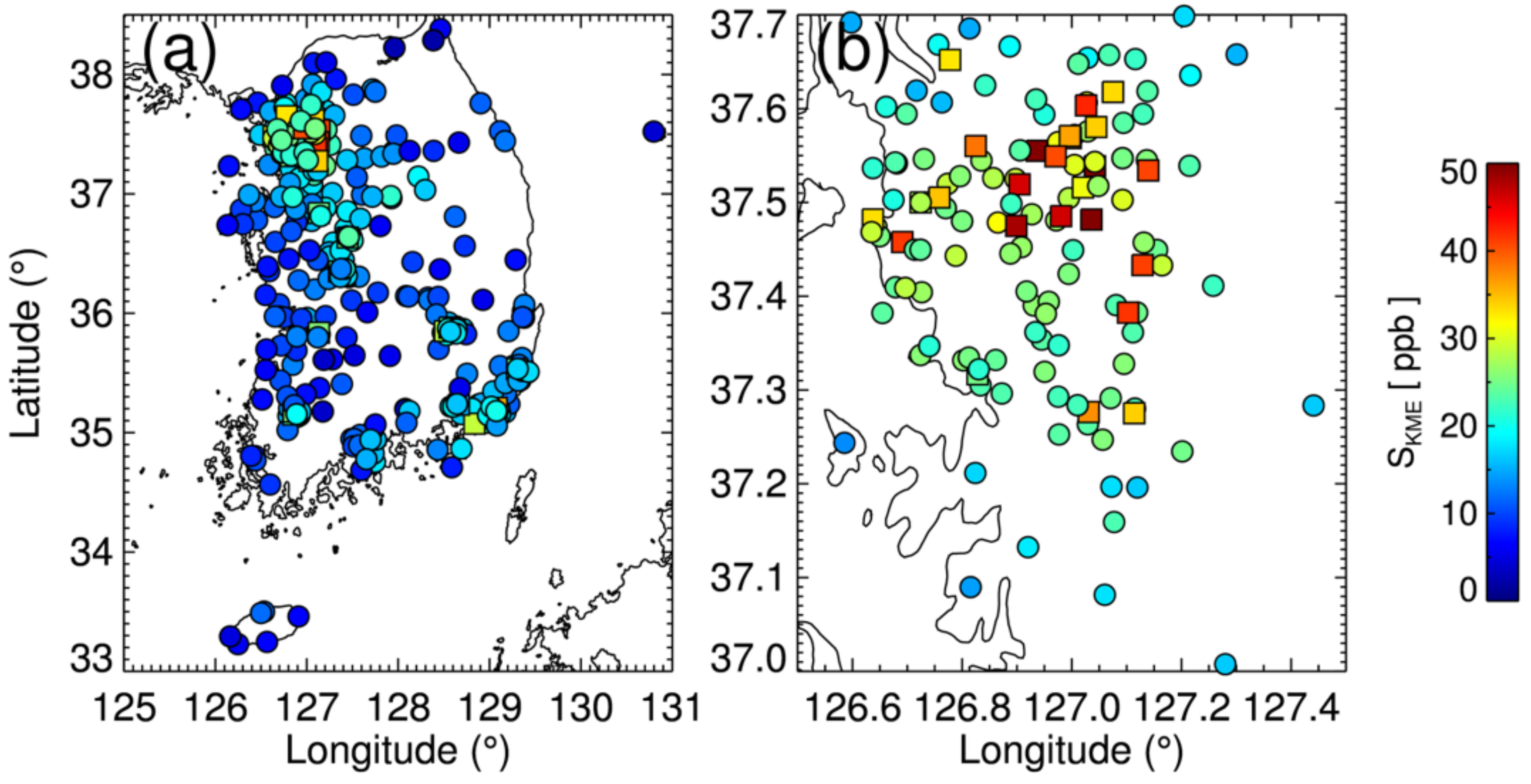
3.1. Spatiotemporal Variations in NO2 from TROPOMI and Ground Network

Figure 1a shows the annual mean value of the NO2 surface mixing ratio from the KME network (SKME) over South Korea, and panel (b) shows the values over the Seoul metropolitan area. The KME network is widely distributed over urban areas, particularly in cities of the Seoul metropolitan area, as shown in Figure 1b. The NO2 mixing ratio measured at roadside stations is 2–3 times higher than that at ambient monitoring stations nearby, which can result in significant variations in NO2 within a TROPOMI footprint (compare values of squares and circles in Figure 1b). However, the stations of SKME are relatively sparse over rural regions, particularly over East and Southwest Korea, where the TROPOMI data can efficiently complement the SKME data.
Figure 2a shows the mean values of the tropospheric NO2 column amounts from TROPOMI (CTROPOMI) for 2019 over South Korea, binned to a comparable resolution of the TROPOMI (0.05° × 0.05° horizontal grid); panel (b) shows the values over the Seoul metropolitan area. More than half the Korean population (~26 million) is distributed near the Seoul metropolitan area, which results in a significant amount of NO2 over this area, as shown in Figure 2a. Dense populations in the city of Busan (~3.4 million) and Ulsan (~1.2 million) along with active ship transport along the southeastern coastal areas resulted in high loadings of CTROPOMI. The populations of Danyang (~37,000) and Gwangyang (~154,000) are relatively low. However, these cities were found to be exposed to moderate loadings of NO2 (0.4–0.5 DU), which can be attributed to a large cement quarry in the Danyang and Industrial Complex in Gwangyang. Daegu is one of the largest cities in South Korea, with a population over 2.4 million located in a basin; it also showed a moderate level of CTROPOMI (~0.4 DU), as shown in Figure 2a. Panel (b) of Figure 2 focuses on the Seoul metropolitan area; the CTROPOMI shows high values throughout the area (0.5–0.8 DU). The CTROPOMI over Seoul was particularly high, followed by those over Sungnam and Suwon. In general, the TROPOMI detects significant sources of NO2 with a high spatial resolution (~5 km) throughout South Korea, which is a key input for epidemiological studies.
As a qualitative comparison of temporal variations in TROPOMI and in-situ measurements, Figure 3 shows the monthly variations of SKME and CTROPOMI in 2019. The green line with diamonds is obtained by averaging all monthly SKME data (for both day and night), whereas the red line with rectangles is obtained from SKME at the TROPOMI overpass time (~13:30 local time). The blue circles show the monthly mean values of CTROPOMI over KME stations. In general, the monthly values of CTROPOMI show consistent temporal variation with the values of SKME (correlation coefficient, r ~ 0.73), which are low in summer and high in winter, mostly because of the different lifetimes of NO2 in different seasons [62]. However, the SKME at the TROPOMI overpass time (annual mean value of 12.8 ppb) is lower than the 24 h averaged value (annual mean value of 16.5 ppb) by approximately 23%, due to the active oxidation of NO2 and boundary layer development during daytime. For a reliable estimate of the long-term exposure to NO2, sophisticated data assimilations/compensations are necessary, to complement the temporal resolution of TROPOMI.
Weekly variations in NO2 concentrations point to the effects of changes in local emissions from traffic and industrial activities, and chemical reactions with other species [63,64]. Figure 4 shows the differences in CTROPOMI and SKME values on weekdays and weekends (ΔCTROPOMI and ΔSKME) in 2019. Panel (a) shows the ΔCTROPOMI over South Korea and (b) over the Seoul metropolitan area, and panel (c) and (d) are those for ΔSKME. Spatial patterns of the ΔCTROPOMI showed good consistency to the ΔSKME, with its beneficial spatial coverage. ΔCTROPOM and ΔSKME were significant over urban areas (e.g., Seoul, Daegu, Ulsan, and Busan), whereas these were relatively small at Danyang and Gwangyang despite the strong emission sources nearby (compare Figure 1a and Figure 2a to Figure 4a,c). This indicates that high values of the CTROPOMI and SKME over these areas (see Figure 1a and Figure 2a) are more attributable to the industrial sources than local traffic emissions. There was no meaningful spatial pattern of ΔCTROPOMI and ΔSKME over the Seoul metropolitan area unlike in the case of CTROPOMI (compare Figure 1b to Figure 4b,d).

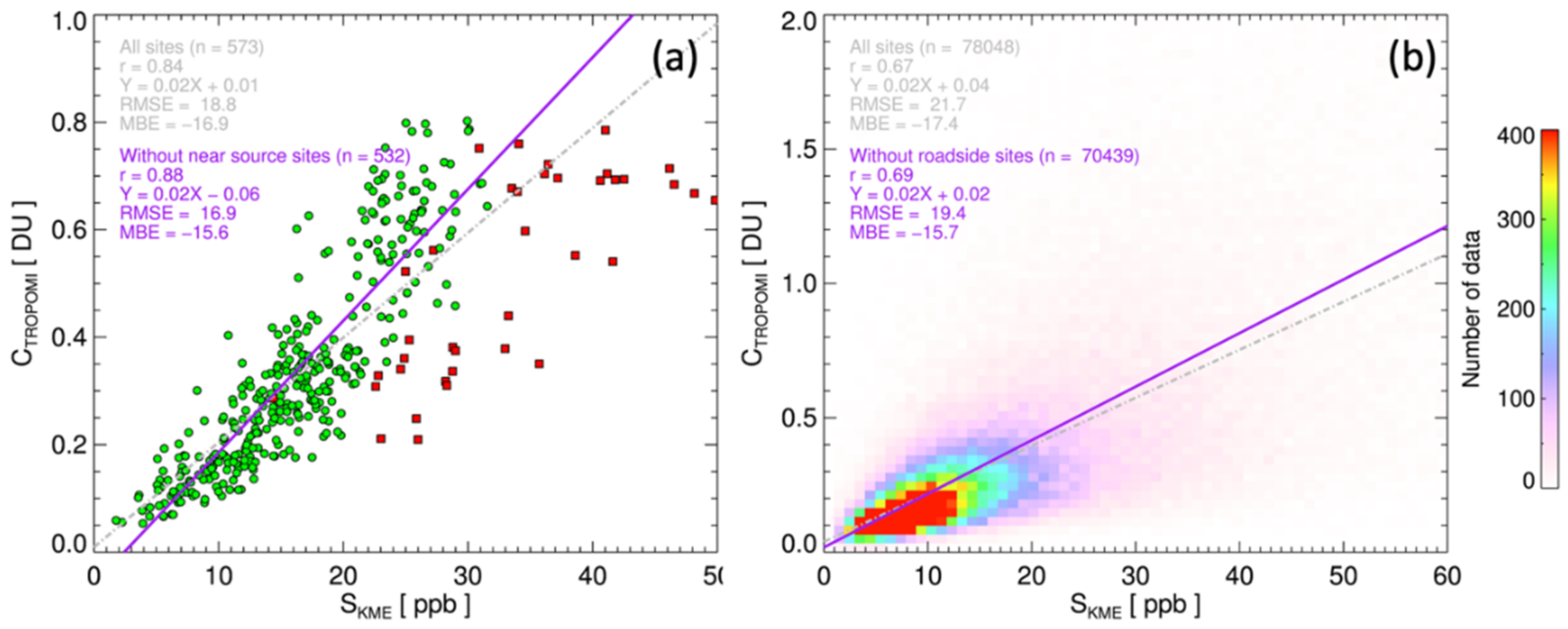
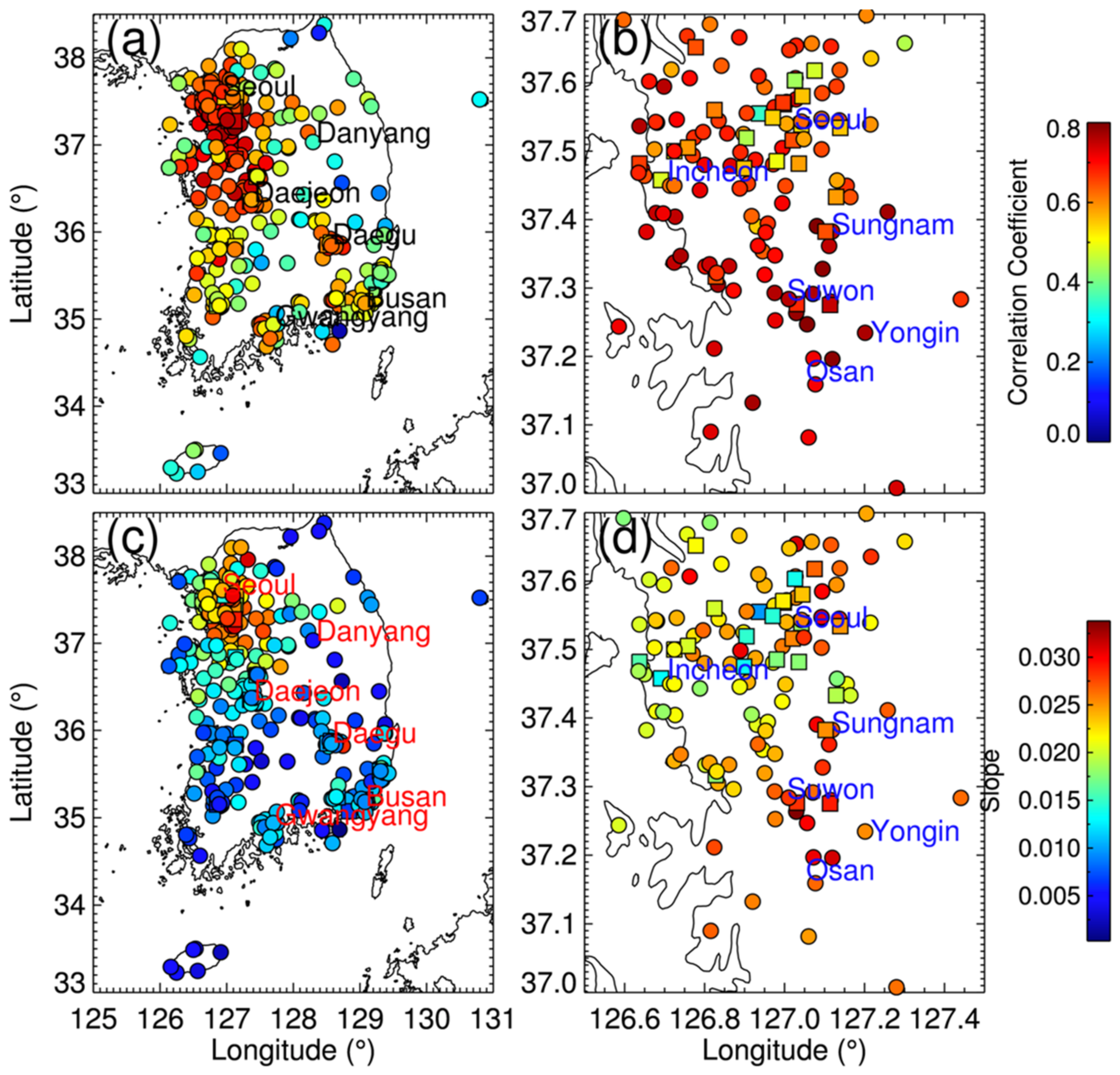
3.2. Correlations of TROPOMI and Surface Measurements of NO2

The annual mean values of CTROPOMI and SKME over the KME stations are compared in Figure 5a. The closest CTROPOMI retrievals to each ground station, of which the distance is less than ±0.025° and quality flag is greater than 0.75, were sampled for use in the calculations. The green circles represent the ambient urban and rural monitoring stations, and the red rectangles indicate the roadside stations. The annual CTROPOMI and SKME values were highly correlated (r = 0.84), particularly over the ambient monitoring sites (r = 0.88). Previous studies [30,32,64] also reported comparable temporal mean values of the satellite retrievals and surface measurements, as random components resulting from measurement errors and spatiotemporal heterogeneities are averaged out. This result repeatedly emphasizes the significance of the TROPOMI data with a high spatial resolution, in estimating long-term exposure to NO2. However, it is to be noted that even TROPOMI with high spatial resolution can underestimate the exposure to NO2 near roads with heavy traffic (or other point sources), without any means of compensation. Assimilating CTROPOMI with land-use data can improve accuracy in the determination of long-term exposure near sources of NO2 [31]. Figure 5b compares all spatiotemporally coincident CTROPOMI and SKME in 2019, which fall within ±0.025° of the ground stations and ±30 min of the TROPOMI overpass time. The correlation between CTROPOMI and SKME (r = 0.67) in this panel also shows statistical values comparable with those of previous studies [32,64]; the correlation is lower than for the annual mean values at the KME stations compared in panel (a). A higher correlation was also observed for ambient monitoring stations excluding roadside sites (r = 0.69).
Figure 6 shows the correlation coefficients and slopes between CTROPOMI and SKME at each KME station for 2019. Strong light absorption by large amounts of NO2 over urban areas results in high retrieval sensitivity in the TROPOMI measurements, which in turn results in higher correlations (see Figure 6a). In the Seoul metropolitan area, the correlations over stations in Seoul were relatively lower than those over southern cities (e.g., Sungnam, Suwon, Yongin, and Osan), particularly over the roadside stations, as shown in Figure 6b. This can be attributed to the higher spatiotemporal variability of NO2 over Seoul than in other cities in the area. The correlations over the roadside stations in the southern cities of the Seoul metropolitan area were high, comparable to the nearby ambient stations. During the dispersion/transport of NO2 from Seoul to these cities, NO2 is well mixed within the air masses, which may result in a spatially homogeneous distribution of NO2. In addition, the local traffic in these cities is relatively lower than that in Seoul, which results in less impact on the spatial variabilities; annual mean values of the NO2 mixing ratio over the roadside stations in these cities are lower than those over Seoul (see Figure 2b). These combined effects may lead to the high correlations between CTROPOMI and SKME over the southern cities of the Seoul metropolitan area.
The slopes shown in panels c and d are calculated using SKME on the x-axis and CTROPOMI on the y-axis, as a unit of DU ppb−1. For a similar level of correlation, the slope indicates the statistical sensitivity of CTROPOMI to SKME, which is associated with the vertical profile of NO2. The slopes in the Seoul metropolitan areas were low along the coastline including at Incheon, which can partially be attributed to complicated boundary layer processes, as shown in Figure 6d. Note that the correlations between CTROPOMI and SKME at different sites in the Seoul metropolitan area are comparable (see Figure 6b). Current AMF calculations of the CTROPOMI may not fully consider the spatial variabilities of small-scale boundary layer processes because the spatial resolution of the TM5-MP model is 1° × 1° [55], which is larger than the whole domain of Figure 6d.

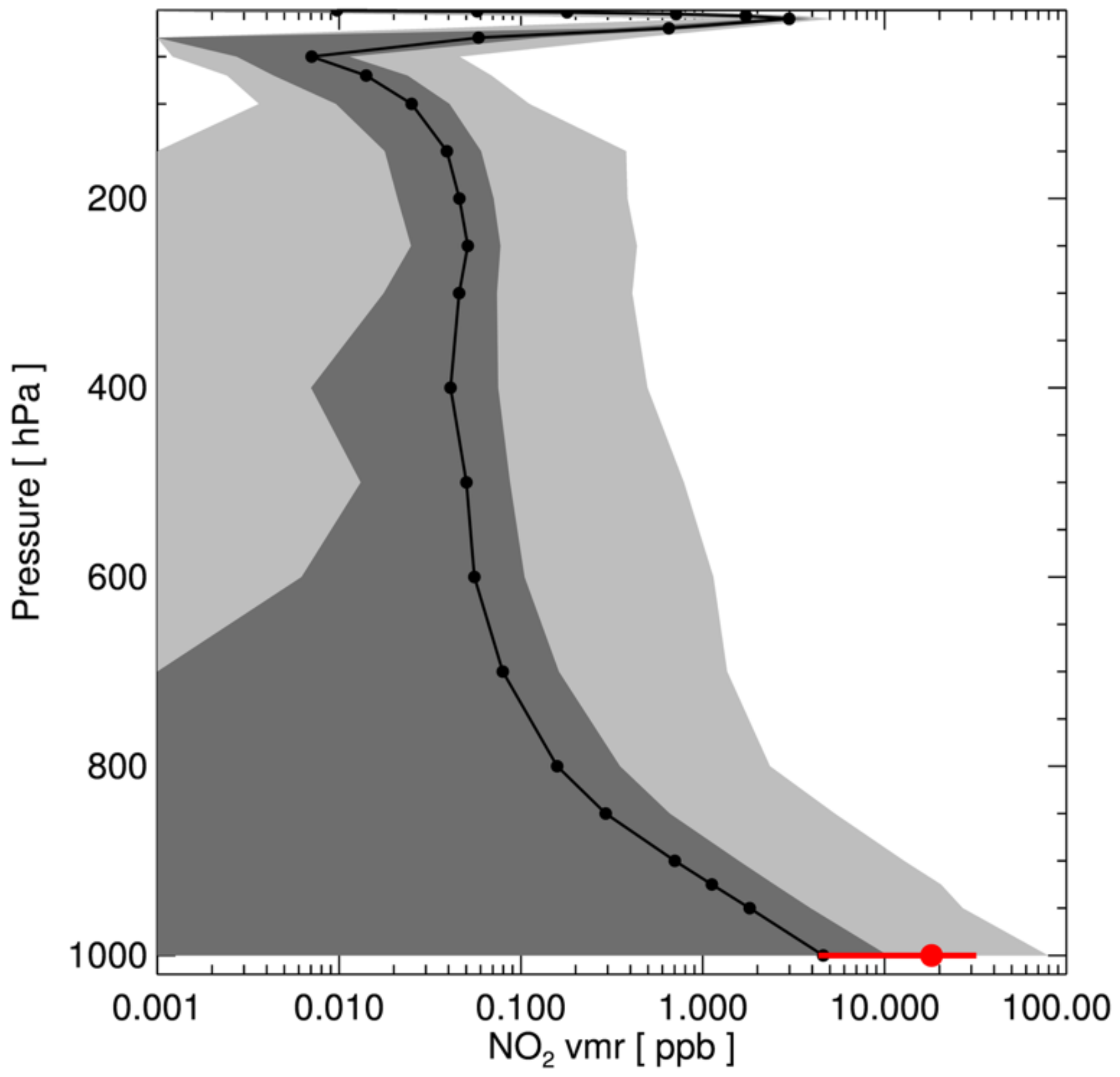
3.3. Estimation of Surface NO2 Mixing Ratio from the TROPOMI Retrievals

To estimate surface air quality from satellite data, vertical profiles of target species are essential [29]. As the EAC4 provides total column and profile of NO2, we separated tropospheric fraction (CEAC4) by integrating the layer amounts from surface to tropopause. For consistency with the CTROPOMI algorithm [51], we followed the definition of thermal tropopause, and estimated boundary levels from the temperature profile of EAC4. However, previous studies reported that other definitions (e.g., dynamical tropopause) would not result in meaningful differences for NO2 [65]. Different atmospheric profile simulations in the EAC4 and TM5-runs for the CTROPOMI may result in additional artifacts for the comparison [66]. For simplicity, such impacts are not considered in the present study. However, we expect biases due to the different averaging kernels are not significant, since the CAMS model system utilizes an identical chemical mechanism (i.e., a modified and extended version of the CB05 [67]) with the TM5 [68] for the AMF calculations. In addition, we assumed that the ratio of SEAC4 to CEAC4 is relatively more accurate than their absolute values, as some of the systematic biases (e.g., emission inventory) are canceled out. We sampled the NO2 profile from the closest pixel of EAC4 at the overpass time of TROPOMI, then the ratio of SEAC4 to CEAC4 was multiplied by CTROPOMI to estimate the surface-level mixing ratio of NO2 from TROPOMI as
S T R O P O M I = S E A C 4 C E A C 4 C T R O P O M I ,
where all parameters are as described in Table 2. The mean values of the NO2 mixing ratio at each layer from EAC4 are shown in Figure 7 (black line with circles). The dark grey area presents ±𝜎 (standard deviation), and the light grey area shows the data range (minimum and maximum values) at each level. The mean and standard deviation of surface NO2 mixing ratio from the EAC4 (4.6 ± 5.8 ppb) were lower than those of the SKME (18.1 ± 13.8 ppb), which is mostly due to the nature of coverage of the KME network; most of the ground stations are located near urban areas or large emission sources, whereas the EAC4 covers the entire region (longitudes from 125° to 131°, and latitudes from 33° to 39°).
Figure 8a compares the annual mean values of STROPOMI and SKME over the KME stations. The correlation coefficient for all ground sites was 0.82, whereas that for ambient stations (other than roadside sites) was 0.86. The STROPOMI underestimated the surface nitrogen values by approximately 30% for the ambient stations (the slope was 0.71, and the intercept was −1.26), and the low bias was greater when the roadside sites were included (the slope was 0.56 and intercept was 0.83). Lamsal et al. [69] combined the OMI and GEOS-Chem (Goddard Earth Observing System Chemistry: 2° × 2.5° horizontal resolution) profiles to estimate the surface NO2 mixing ratio over North America and reported low biases of up to 36%. Bechle et al. [30] also reported low biases of the NO2 mixing ratio over Southern California; 31% when combining the OMI and Comprehensive Air-Quality Model with extensions (CAMx) with 2 × 2 km horizontal resolution and 60% when combining the OMI and GEOS-Chem profiles. Cooper et al. [36] also presented low biases of the TROPOMI NO2 compared to in-situ measurements over the United States based on similar comparison of this study (slope = 0.46, r = 0.71). However, they improved the slope (1.02) after applying their algorithm, which accounts for the spatial resolution of TROPOMI and realistic mixing assumptions in the boundary layer [36]. A major fraction of the low biases in this study can be attributed to the uncertainties in the CTROPOMI (negative biases of approximately 22% [59]), and the spatial heterogeneity of NO2 within the TROPOMI and TM5-MP grids. Lower correlation coefficients (r = 0.65 and 0.63 for ambient stations and all stations, respectively) with comparable slopes (slope = 0.65 and 0.60 for ambient stations and all stations, respectively) to those shown in Figure 8a were identified from a comparison of all coincident data as shown in Figure 8b. The results suggest that compensation for these low biases is essential for estimating both short-term and long-term exposure to NO2 in South Korea.
Figure 9 shows the average ratio of STROPOMI to SKME over each ground station in 2019. The STROPOMI generally underestimates surface NO2—particularly at rural stations in the western part of the Korean peninsula—by about 30–60% (see Figure 9a). The low bias was relatively small over the Seoul metropolitan area, Busan, and Gwangyang. Considering the ambient monitoring stations in the Seoul metropolitan area (Figure 9b), the STROPOMI underestimates surface NO2 near the coastal areas around Incheon, as compared to the inland cities (Seoul, Sungnam, Suwan, Osan, Yongin). As discussed with reference to Figure 6, these small-scale variations shown in Figure 9b may be associated with the complicated boundary layer processes along the coastal areas, which need to be investigated in future studies. As expected, the low biases of the STROPOMI were significant at roadside stations, with biases of about 40–60% (see values associated with the squares in Figure 9b).

4. Discussion

For better resolving horizontal variabilities of NO2 using the TROPOMI product, several regional and multi-scale models (e.g., Weather Research and Forecasting-Chemistry [70], Community Multiscale Air Quality Modeling System [71]) can provide high-spatial-resolution of a priori atmospheric profiles which are comparable to or smaller than the TROPOMI’s footprint. Griffin et al. [33] utilized a 10 × 10 km horizontal resolution of GEM-MACH (Global Environmental Multiscale-Modelling Air-quality and Chemistry) simulations to improve AMF estimations. Cooper et al. [36] used moderate horizontal-resolution (0.25° × 0.3125°) of GEOS-Chem (Goddard Earth Observing System-Chemistry [72]) calculations to take account for the different averaging kernels from the operational algorithm, then applied additional correction which significantly improved the low biases of TROPOMI estimates.
For proper calculations of such models, comparable or higher spatial-resolution of emission inventory than that of a model grid is essential. The Regional Emission inventory in ASia (REAS) has provided reliable emission inventory since 1950 with a spatial resolution of 0.25° × 0.25° [73]. The KME annually reports emission inventory of South Korea with a 1 × 1 km resolution but limited to inside the border [74]. However, in our knowledge, emission inventory with a spatial resolution comparable or higher to the CTROPOMI covering East Asia is not available yet. In addition, simulation of small-scale boundary layer processes over coastal areas and complicated terrains are still challenging. As the Korean peninsula is surrounded by ocean and over 70% of the territory is covered with mountains, high-resolution model run may introduce additional complication from the model uncertainties. Intensive field campaigns combined with model simulations over these areas (e.g., Ozone Water-Land Environmental Transition Study [75]) would help to better understand such phenomena. At this moment, the assimilated EAC4 data would provide practical and reliable NO2 profiles despite its coarser resolution than the CTROPOMI, since it is one of the most reliable assimilated NO2 data which are publicly available over globe. In addition, the estimations and assessments in this study is applicable to other regions (e.g., other Asian countries, where in-situ measurements are sparse) as the EAC4 provides relatively uniform quality over globe. Therefore, this study suggests assessments of a minimum capability of TROPOMI to monitor surface NO2 for broader applications.

5. Summary and Conclusions

This study compared the tropospheric column amount of NO2 retrieved from TROPOMI data to in-situ surface measurements over South Korea, for 2019. The surface network consists of 570 stations including 41 roadside stations, providing extensive coverage over urban areas. The spatial distribution of annual mean values of CTROPOMI detected at major and minor source areas of NO2 showed a clear weekday–weekend distinction, particularly over the Seoul metropolitan area. Monthly variations in CTROPOMI and SKME showed good correlation (r ~ 0.73), which were high in winter and low in summer, mostly due to the different lifetimes of NO2 in different seasons. The SKME corresponding to the TROPOMI overpass time was lower than the 24 h averaged value by approximately 23%, owing to the active oxidation of NO2 during daytime.
Coincident measurements of CTROPOMI and SKME showed a moderate correlation (r = 0.67), which is comparable to previous studies in Europe and North America. Their annual mean values at each ground station were highly correlated (r = 0.84), particularly when the roadside stations were not considered (r = 0.88), because random components comprising measurement errors and spatiotemporal heterogeneities were averaged out. However, even TROPOMI with high spatial resolution can underestimate the exposure to NO2 near roads with heavy traffic (or other point sources), which needs to be compensated by other methods (e.g., land-use regression models and data assimilation using high-resolution chemical transport models). The correlations between CTROPOMI and SKME were relatively higher in urban stations than in rural areas.
CTROPOMI was converted to surface mixing ratio (STROPOMI) using the NO2 profile from the EAC4. The annual mean values of STROPOMI were highly correlated with the SKME (r = 0.82), particularly over the ambient monitoring stations (r = 0.86). However, STROPOMI underestimated the values by about 30% for the ambient stations (the slope was 0.71, and intercept was −1.26), and the low bias was greater when the roadside sites were included (the slope was 0.56 and intercept was 0.83). Uncertainties in the CTROPOMI (negative biases of approximately 22%) and spatial heterogeneity of NO2 within the TROPOMI and TM5-MP grids can be the reason for a major fraction of the low biases. The underestimation of STROPOMI was significant over rural stations in the western part of the Korean peninsula at about 30–60%, whereas it was relatively small over larger urban areas. Over the ambient monitoring stations in the Seoul metropolitan area, the low bias of STROPOMI was more significant near the coastal areas than inland cities, which may be associated with the complicated boundary layer processes along the coastline. As expected, the underestimation of the STROPOMI was significant over roadside sites by approximately 40–60%.

Author Contributions

Conceptualization, methodology, formal analysis, investigation, resources, data curation, writing, and editing by U.J. Software, validation, resources, writing and editing, visualization, and funding acquisition by H.H. All authors have read and agreed to the published version of the manuscript.

Funding

This research was supported by the National Institute of Environmental Research (NIER) of the Ministry of Environment, Republic of Korea (grant no. NIER-2021-01-01-052).

Institutional Review Board Statement

Not applicable.

Informed Consent Statement

Not applicable.

Data Availability Statement

The TROPOMI data are available at http://www.tropomi.eu/data-products/data-access (accessed on 21 January 2021), and the EAC4 data are from https://ads.atmosphere.copernicus.eu (accessed on 21 January 2021). We obtained the KME ground measurements from https://www.airkorea.or.kr (accessed on 21 January 2021).

Acknowledgments

The authors appreciate ESA and NASA for providing the TROPOMI and EAC4 data, and thank the Korean Ministry of Environment for the in-situ NO2 data.

Conflicts of Interest

The authors declare no conflict of interest. The funder had no role in the design of the study; collection, analyses, or interpretation of data; in the writing of the manuscript; or in the decision to publish the results.

References

  1. WHO. Review of Evidence on Health Aspects of Air Pollution, RE-VIHAAP Project; World Health Organization, WHO Regional Office for Europe: Copenhagen, Denmark, 2013. [Google Scholar]
  2. US EPA. Nitrogen Dioxide (NO2) Pollution. Available online: https://www.epa.gov/no2-pollution (accessed on 1 January 2021).
  3. Beelen, R.; Hoek, G.; Brandt, P.A.V.D.; Goldbohm, R.A.; Fischer, P.; Schouten, L.J.; Jerrett, M.; Hughes, E.; Armstrong, B.; Brunekreef, B. Long-Term Effects of Traffic-Related Air Pollution on Mortality in a Dutch Cohort (NLCS-AIR Study). Environ. Health Perspect. 2008, 116, 196–202. [Google Scholar] [CrossRef] [PubMed]
  4. Filleul, L.; Rondeau, V.; Vandentorren, S.; le Moual, N.; Cantagrel, A.; Annesi-Maesano, I.; Charpin, D.; Declercq, C.; Neukirch, F.; Paris, C.; et al. Twenty five year mortality and air pollution: Results from the French PAARC survey. Occup. Environ. Med. 2005, 62, 453–460. [Google Scholar] [CrossRef] [PubMed] [Green Version]
  5. Castellsague, J.; Sunyer, J.; Saez, M.; Anto, J.M. Short-term association between air pollution and emergency room visits for asthma in Barcelona. Thorax 1995, 50, 1051–1056. [Google Scholar] [CrossRef] [PubMed] [Green Version]
  6. Gauderman, W.J.; Avol, E.; Lurmann, F.; Kuenzli, N.; Gilliland, F.; Peters, J.; McConnell, R. Childhood Asthma and Exposure to Traffic and Nitrogen Dioxide. Epidemiology 2005, 16, 737–743. [Google Scholar] [CrossRef]
  7. Chen, R.; Samoli, E.; Wong, C.M.; Huang, W.; Wang, Z.; Chen, B.; Kan, H. CAPES Collaborative Group: Associations between short-term exposure to nitrogen dioxide and mortality in 17 Chinese cities: The China Air Pollution and Health Effects Study (CAPES). Environ. Int. 2012, 45, 32–38. [Google Scholar] [CrossRef]
  8. Crutzen, P.J. The Role of NO and NO2 in the Chemistry of the Troposphere and Stratosphere. Annu. Rev. Earth Planet. Sci. 1979, 7, 443–472. [Google Scholar] [CrossRef]
  9. Liu, S.C.; Trainer, M.; Fehsenfeld, F.C.; Parrish, D.D.; Williams, E.J.; Fahey, D.W.; Hübler, G.; Murphy, P.C. Ozone production in the rural troposphere and the implications for regional and global ozone distributions. J. Geophys. Res. Space Phys. 1987, 92, 4191–4207. [Google Scholar] [CrossRef]
  10. Han, S.; Bian, H.; Feng, Y.; Liu, A.; Li, X.; Zeng, F.; Zhang, X. Analysis of the relationship between O3, NO and NO2 in Tianjin, China. Aerosol Air Qual. Res. 2011, 11, 128–139. [Google Scholar] [CrossRef] [Green Version]
  11. Notholt, J.; Hjorth, J.; Raes, F. Formation of HNO2 on aerosol surfaces during foggy periods in the presence of NO and NO2. Atmos. Environ. Part A Gen. Top. 1992, 26, 211–217. [Google Scholar] [CrossRef]
  12. Squizzato, S.; Masiol, M.; Brunelli, A.; Pistollato, S.; Tarabotti, E.; Rampazzo, G.; Pavoni, B. Factors determining the formation of secondary inorganic aerosol: A case study in the Po Valley (Italy). Atmos. Chem. Phys. Discuss. 2013, 13, 1927–1939. [Google Scholar] [CrossRef] [Green Version]
  13. Hoek, G.; Beelen, R.; de Hoogh, K.; Vienneau, D.; Gulliver, J.; Fischer, P.; Briggs, D. A review of land-use regression models to assess spatial variation of outdoor air pollution. Atmos. Environ. 2008, 42, 7561–7578. [Google Scholar] [CrossRef]
  14. Liu, F.; Beirle, S.; Zhang, Q.; Dörner, S.; He, K.; Wagner, T. NOx lifetimes and emissions of cities and power plants in polluted background estimated by satellite observations. Atmos. Chem. Phys. 2016, 16, 5283–5298. [Google Scholar] [CrossRef] [Green Version]
  15. Laughner, J.L.; Cohen, R.C. Direct observation of changing NOx lifetime in North American cities. Science 2019, 366, 723–727. [Google Scholar] [CrossRef]
  16. Ielpo, P.; Mangia, C.; Marra, G.; Comite, V.; Rizza, U.; Uricchio, V.; Fermo, P. Outdoor spatial distribution and indoor levels of NO2 and SO2 in a high environmental risk site of the South Italy. Sci. Total Environ. 2019, 648, 787–797. [Google Scholar] [CrossRef]
  17. United States Environmental Protection Agency. Available online: https://epa.gov (accessed on 1 January 2021).
  18. European Environmental Agency. Available online: https://www.eea.europa.eu/ (accessed on 1 January 2021).
  19. Air, Korea. Available online: https://www.airkorea.or.kr (accessed on 1 January 2021).
  20. Briggs, D.J.; Collins, S.; Elliott, P.; Fischer, P.; Kingham, S.; Lebret, E.; Pryl, K.; Van Reeuwijk, H.; Smallbone, K.; Van Der Veen, A. Mapping urban air pollution using GIS: A regression-based approach. Int. J. Geogr. Inf. Sci. 1997, 11, 699–718. [Google Scholar] [CrossRef] [Green Version]
  21. Burrows, J.P.; Weber, M.; Buchwitz, M.; Rozanov, V.; Ladstätter-Weißenmayer, A.; Richter, A.; DeBeek, R.; Hoogen, R.; Bramstedt, K.; Eichmann, K.-U.; et al. The Global Ozone Monitoring Experiment (GOME): Mission Concept and First Scientific Results. J. Atmos. Sci. 1999, 56, 151–175. [Google Scholar] [CrossRef]
  22. Munro, R.; Lang, R.; Klaes, D.; Poli, G.; Retscher, C.; Lindstrot, R. The GOME-2 instrument on the metop series of satellites: Instrument design, calibration, and level 1 data processing-an overview. Atmos. Meas. Tech. 2016, 9, 1279–1301. [Google Scholar] [CrossRef] [Green Version]
  23. Bovensmann, H.; Burrows, J.P.; Buchwitz, M.; Frerick, J.; Noël, S.; Rozanov, V.V.; Chance, K.V.; Goede, A.P.H. SCIAMACHY: Mission Objectives and Measurement Modes. J. Atmos. Sci. 1999, 56, 127–150. [Google Scholar] [CrossRef] [Green Version]
  24. Levelt, P.; Oord, G.V.D.; Dobber, M.; Malkki, A.; Visser, H.; De Vries, J.; Stammes, P.; Lundell, J.; Saari, H. The ozone monitoring instrument. IEEE Trans. Geosci. Remote Sens. 2006, 44, 1093–1101. [Google Scholar] [CrossRef]
  25. Boersma, K.F.; Eskes, H.J.; Richter, A.; de Smedt, I.; Lorente, A.; Beirle, S.; van Geffen, J.H.G.M.; Zara, M.; Peters, E.; van Roozendael, M.; et al. Improving algorithms and uncertainty estimates for satellite NO2 retrievals: Results from the quality assurance for the essential climate variables (QA4ECV) project. Atmos. Meas. Tech. 2018, 11, 6651–6678. [Google Scholar] [CrossRef] [Green Version]
  26. Kim, J.; Jeong, U.; Ahn, M.-H.; Kim, J.H.; Park, R.J.; Lee, H.; Song, C.H.; Choi, Y.-S.; Lee, K.-H.; Yoo, J.-M.; et al. New Era of Air Quality Monitoring from Space: Geostationary Environment Monitoring Spectrometer (GEMS). Bull. Am. Meteorol. Soc. 2020, 101, E1–E22. [Google Scholar] [CrossRef] [Green Version]
  27. Brauer, M.; Amann, M.; Burnett, R.T.; Cohen, A.; Dentener, F.; Ezzati, M.; Henderson, S.B.; Krzyzanowski, M.; Martin, R.V.; van Dingenen, R.; et al. Exposure Assessment for Estimation of the Global Burden of Disease Attributable to Outdoor Air Pollution. Environ. Sci. Technol. 2011, 46, 652–660. [Google Scholar] [CrossRef] [Green Version]
  28. Van Donkelaar, A.; Martin, R.V.; Brauer, M.; Kahn, R.; Levy, R.; Verduzco, C.; Villeneuve, P.J. Global Estimates of Ambient Fine Particulate Matter Concentrations from Satellite-Based Aerosol Optical Depth: Development and Application. Environ. Health Perspect. 2010, 118, 847–855. [Google Scholar] [CrossRef] [Green Version]
  29. Martin, R.V. Satellite remote sensing of surface air quality. Atmos. Environ. 2008, 42, 7823–7843. [Google Scholar] [CrossRef]
  30. Bechle, M.J.; Millet, D.B.; Marshall, J.D. Remote sensing of exposure to NO2: Satellite versus ground-based measurement in a large urban area. Atmos. Environ. 2013, 69, 345–353. [Google Scholar] [CrossRef]
  31. Anand, J.S.; Monks, P.S. Estimating daily surface NO2 concentrations from satellite data—A case study over Hong Kong using land use regression models. Atmos. Chem. Phys. Discuss. 2017, 17, 8211–8230. [Google Scholar] [CrossRef] [Green Version]
  32. Ialongo, I.; Virta, H.; Eskes, H.; Hovila, J.; Douros, J. Comparison of TROPOMI/Sentinel-5 Precursor NO2 observations with ground-based measurements in Helsinki. Atmos. Meas. Tech. 2020, 13, 205–218. [Google Scholar] [CrossRef] [Green Version]
  33. Griffin, D.; Zhao, X.; McLinden, C.A.; Boersma, F.; Bourassa, A.; Dammers, E.; Degenstein, D.; Eskes, H.; Fehr, L.; Fioletov, V.; et al. High-Resolution Mapping of Nitrogen Dioxide With TROPOMI: First Results and Validation Over the Canadian Oil Sands. Geophys. Res. Lett. 2019, 46, 1049–1060. [Google Scholar] [CrossRef] [Green Version]
  34. Zheng, Z.; Yang, Z.; Wu, Z.; Marinello, F. Spatial Variation of NO2 and Its Impact Factors in China: An Application of Sentinel-5P Products. Remote Sens. 2019, 11, 1939. [Google Scholar] [CrossRef] [Green Version]
  35. Goldberg, D.L.; Anenberg, S.C.; Kerr, G.H.; Mohegh, A.; Lu, Z.; Streets, D.G. TROPOMI NO2 in the United States: A Detailed Look at the Annual Averages, Weekly Cycles, Effects of Temperature, and Correlation with Surface NO2 Concentrations. Earth’s Future 2021, 9, e2020EF001665. [Google Scholar] [CrossRef]
  36. Cooper, M.J.; Martin, R.V.; McLinden, C.A.; Brook, J.R. Inferring ground-level nitrogen dioxide concentrations at fine spatial resolution applied to the TROPOMI satellite instrument. Environ. Res. Lett. 2020, 15, 104013. [Google Scholar] [CrossRef]
  37. Kim, N.K.; Kim, Y.P.; Morino, Y.; Kurokawa, J.-I.; Ohara, T. Verification of NOx emission inventory over South Korea using sectoral activity data and satellite observation of NO2 vertical column densities. Atmos. Environ. 2013, 77, 496–508. [Google Scholar] [CrossRef]
  38. Judd, L.M.; Al-Saadi, J.A.; Valin, L.C.; Pierce, R.B.; Yang, K.; Janz, S.J.; Kowalewski, M.G.; Szykman, J.J.; Tiefengraber, M.; Mueller, M. The Dawn of Geostationary Air Quality Monitoring: Case Studies from Seoul and Los Angeles. Front. Environ. Sci. 2018, 6, 85. [Google Scholar] [CrossRef] [PubMed]
  39. Jeong, U.; Kim, J.; Lee, H.; Jung, J.; Kim, Y.J.; Song, C.H.; Koo, J.-H. Estimation of the contributions of long range transported aerosol in East Asia to carbonaceous aerosol and PM concentrations in Seoul, Korea using highly time resolved measurements: A PSCF model approach. J. Environ. Monit. 2011, 13, 1905–1918. [Google Scholar] [CrossRef] [PubMed]
  40. Kim, M.; Kim, J.; Jeong, U.; Kim, W.; Hong, H.; Holben, B.; Eck, T.F.; Lim, J.H.; Song, C.K.; Lee, S.; et al. Aerosol optical properties derived from the DRAGON-NE Asia campaign, and implications for a single-channel algorithm to retrieve aerosol optical depth in spring from Meteorological Imager (MI) on-board the Communication, Ocean, and Meteorological Satellite (COMS). Atmos. Chem. Phys. Discuss. 2016, 16, 1789–1808. [Google Scholar] [CrossRef] [Green Version]
  41. Leitao, J.; Richter, A.; Vrekoussis, M.; Kokhanovsky, A.; Zhang, Q.J.; Beekmann, M.; Burrows, J.P. On the improvement of NO2 satellite retrievals—Aerosol impact on the airmass factors. Atmos. Meas. Tech. 2010, 3, 475–493. [Google Scholar] [CrossRef] [Green Version]
  42. Lin, J.-T.; Martin, R.V.; Boersma, K.F.; Sneep, M.; Stammes, P.; Spurr, R.; Wang, P.; Van Roozendael, M.; Clémer, K.; Irie, H. Retrieving tropospheric nitrogen dioxide from the Ozone Monitoring Instrument: Effects of aerosols, surface reflectance anisotropy, and vertical profile of nitrogen dioxide. Atmos. Chem. Phys. 2014, 14, 1441–1461. [Google Scholar] [CrossRef] [Green Version]
  43. Hong, H.; Lee, H.; Kim, J.; Jeong, U.; Ryu, J.; Lee, D.S. Investigation of Simultaneous Effects of Aerosol Properties and Aerosol Peak Height on the Air Mass Factors for Space-Borne NO2 Retrievals. Remote Sens. 2017, 9, 208. [Google Scholar] [CrossRef] [Green Version]
  44. NIER (National Institute of Environmental Research). Annual Report of Air Quality in Korea; Ministry of the Environment: Sejongsi, Korea, 2019.
  45. Inness, A.; Ades, M.; Agustí-Panareda, A.; Barré, J.; Benedictow, A.; Blechschmidt, A.-M.; Dominguez, J.J.; Engelen, R.; Eskes, H.; Flemming, J.; et al. The CAMS reanalysis of atmospheric composition. Atmos. Chem. Phys. Discuss. 2019, 19, 3515–3556. [Google Scholar] [CrossRef] [Green Version]
  46. Razinger, M.; Remy, S.; Schulz, M.; Suttie, M. 1KNMI: Algorithm Theoretical Basis Document for the TROPOMI L01b Data Processor, S5P-KNMI-L01B-0009-SD, Koninklijk Nederlands Meteorologisch Instituut (KNMI), CI-6480-ATBD, Issue 8.0.0. 2017. Available online: https://sentinels.copernicus.eu/documents/247904/2476257/Sentinel-5P-TROPOMI-Level-1B-ATBD (accessed on 21 January 2021).
  47. Veefkind, J.P.; Aben, I.; McMullan, K.; Förster, H.; De Vries, J.; Otter, G.; Claas, J.; Eskes, H.J.; De Haan, J.F.; Kleipool, Q.; et al. TROPOMI on the ESA Sentinel-5 Precursor: A GMES mission for global observations of the atmospheric composition for climate, air quality and ozone layer applications. Remote Sens. Environ. 2012, 120, 70–83. [Google Scholar] [CrossRef]
  48. Kleipool, Q.; Ludewig, A.; Babić, L.; Bartstra, R.; Braak, R.; Dierssen, W.; Dewitte, P.-J.; Kenter, P.; Landzaat, R.; Leloux, J.; et al. Pre-launch calibration results of the TROPOMI payload on-board the Sentinel-5 Precursor satellite. Atmos. Meas. Tech. 2018, 11, 6439–6479. [Google Scholar] [CrossRef] [Green Version]
  49. Boersma, K.F.; Eskes, H.J.; Dirksen, R.J.; van der A, R.J.; Veefkind, J.P.; Stammes, P.; Huijnen, V.; Kleipool, Q.; Sneep, M. An improved tropospheric NO2 column retrieval algorithm for the Ozone Monitoring Instrument. Atmos. Meas. Tech. 2011, 4, 1905–1928. [Google Scholar] [CrossRef] [Green Version]
  50. Van Geffen, J.H.G.M.; Boersma, K.F.; van Roozendael, M.; Hendrick, F.; Mahieu, E.; de Smedt, I.; Sneep, M.; Veefkind, J.P. Improved spectral fitting of nitrogen dioxide from OMI in the 405–465 nm window. Atmos. Meas. Tech. 2015, 8, 1685–1699. [Google Scholar] [CrossRef] [Green Version]
  51. Van Geffen, J.H.G.M.; Eskes, H.J.; Boersma, K.F.; Maasakkers, J.D.; Veefkind, J.P. TROPOMI ATBD of the Total and Tropospheric NO2 Data Products 2019. Available online: https://sentinel.esa.int/documents/247904/2476257/Sentinel-5P-TROPOMI-ATBD-NO2-data-products (accessed on 25 January 2021).
  52. Zara, M.; Boersma, K.F.; De Smedt, I.; Richter, A.; Peters, E.; van Geffen, J.H.G.M.; Beirle, S.; Wagner, T.; Van Roozendael, M.; Marchenko, S.; et al. Improved slant column density retrieval of nitrogen dioxide and formaldehyde for OMI and GOME-2A from QA4ECV: Intercomparison, uncertainty characterisation, and trends. Atmos. Meas. Tech. 2018, 11, 4033–4058. [Google Scholar] [CrossRef] [Green Version]
  53. Platt, U. Differential Optical Absorption Spectroscopy (DOAS), in Air Monitoring by Spectroscopic, Techniques; John Wiley: New York, NY, USA, 1994; pp. 27–84. [Google Scholar]
  54. Platt, U.; Stutz, J. Differential Optical Absorption Spectroscopy: Principles and Applications; Springer Verlag: Berlin/Heidelberg, Germany, 2008. [Google Scholar]
  55. Williams, J.E.; Boersma, K.F.; le Sager, P.; Verstraeten, W.W. The high-resolution version of TM5-MP for optimized satellite retrievals: Description and validation. Geosci. Model Dev. 2017, 10, 721–750. [Google Scholar] [CrossRef] [Green Version]
  56. Kleipool, Q.L.; Dobber, M.R.; de Haan, J.F.; Levelt, P.P. Earth surface reflectance climatology from 3 years of OMI data. J. Geophys. Res. Space Phys. 2008, 113, 18308. [Google Scholar] [CrossRef]
  57. Eskes, H.J.; Eichmann, K.-U. S5P Mission Performance Centre Nitrogen Dioxide; Readme L2; KNMI: DeBilt, The Netherlands, 2019. [Google Scholar]
  58. Lambert, J.-C.; Keppens, A.; Hubert, D.; Langerock, B.; Eichmann, K.-U.; Kleipool, Q.; Sneep, M.; Verhoelst, T.; Wagner, T.; Weber, M.; et al. Quarterly Validation Report of the Copernicus Sentinel-5 Precursor Operational Data Products, Issue # 02, Version 02.0.2, 109 pp, April 2019. Available online: http://www.tropomi.eu/sites/default/files/files/publicS5P-MPC-IASB-ROCVR-02.0.2-20190411_FINAL.pdf (accessed on 27 January 2021).
  59. Sentinel-5 Precursor Mission Performance Centre Validation Facility. Available online: https://mpc-vdaf.tropomi.eu/ (accessed on 27 January 2021).
  60. Inness, A.; Blechschmidt, A.-M.; Bouarar, I.; Chabrillat, S.; Crepulja, M.; Engelen, R.J.; Eskes, H.; Flemming, J.; Gaudel, A.; Hendrick, F.; et al. Data assimilation of satellite-retrieved ozone, carbon monoxide and nitrogen dioxide with ECMWF’s Composition-IFS. Atmos. Chem. Phys. 2015, 15, 5275–5303. [Google Scholar] [CrossRef] [Green Version]
  61. Judd, L.M.; Al-Saadi, J.A.; Janz, S.J.; Kowalewski, M.G.; Pierce, R.B.; Szykman, J.J.; Valin, L.C.; Swap, R.; Cede, A.; Mueller, M.; et al. Evaluating the impact of spatial resolution on tropospheric NO2 column comparisons within urban areas using high-resolution airborne data. Atmos. Meas. Tech. 2019, 12, 6091–6111. [Google Scholar] [CrossRef] [Green Version]
  62. Shah, V.; Jacob, D.J.; Li, K.; Silvern, R.F.; Zhai, S.; Liu, M.; Lin, J.; Zhang, Q. Effect of changing NOx lifetime on the seasonality and long-term trends of satellite-observed tropospheric NO2 columns over China. Atmos. Chem. Phys. Discuss. 2020, 20, 1483–1495. [Google Scholar] [CrossRef] [Green Version]
  63. Valin, L.C.; Russell, A.R.; Cohen, R.C. Chemical feedback effects on the spatial patterns of the NOx weekend effect: A sensitivity analysis. Atmos. Chem. Phys. Discuss. 2014, 14, 1–9. [Google Scholar] [CrossRef] [Green Version]
  64. Cersosimo, A.; Serio, C.; Masiello, G. TROPOMI NO2 Tropospheric Column Data: Regridding to 1 km Grid-Resolution and Assessment of their Consistency with in Situ Surface Observations. Remote Sens. 2020, 12, 2212. [Google Scholar] [CrossRef]
  65. Bucsela, E.J.; Krotkov, N.A.; Celarier, E.A.; Lamsal, L.N.; Swartz, W.H.; Bhartia, P.K.; Boersma, K.F.; Veefkind, J.P.; Gleason, J.F.; Pickering, K.E. A new stratospheric and tropospheric NO2 retrieval algorithm for nadir-viewing satellite instruments: Applications to OMI. Atmos. Meas. Tech. 2013, 6, 2607–2626. [Google Scholar] [CrossRef] [Green Version]
  66. Eskes, H.J.; Boersma, K.F. Averaging kernels for DOAS total-column satellite retrievals. Atmos. Chem. Phys. Discuss. 2003, 3, 1285–1291. [Google Scholar] [CrossRef] [Green Version]
  67. CAMx. User’s Guide—Comprehensive Air-Quality Model with Extensions, Version 5.40; ENVIRON International Corporation: Novato, CA, USA, 2011; Available online: http://www.camx.com (accessed on 29 December 2011).
  68. Huijnen, V.; Williams, J.; Van Weele, M.; Van Noije, T.; Krol, M.; Dentener, F.; Segers, A.; Houweling, S.; Peters, W.; De Laat, J.; et al. The global chemistry transport model TM5: Description and evaluation of the tropospheric chemistry version 3.0. Geosci. Model Dev. 2010, 3, 445–473. [Google Scholar] [CrossRef] [Green Version]
  69. Lamsal, L.N.; Martin, R.V.; van Donkelaar, A.; Steinbacher, M.; Celarier, E.A.; Bucsela, E.; Dunlea, E.J.; Pinto, J.P. Ground-level nitrogen dioxide concentrations inferred from the satellite-borne Ozone Monitoring Instrument. J. Geophys. Res. Space Phys. 2008, 113, 16308. [Google Scholar] [CrossRef] [Green Version]
  70. Powers, J.G.; Klemp, J.B.; Skamarock, W.C.; Davis, C.A.; Dudhia, J.; Gill, D.O.; Coen, J.L.; Gochis, D.J.; Ahmadov, R.; Peckham, S.E.; et al. The weather research and forecasting model: Overview, System Efforts, and Future Directions. Bull. Am. Meteorol. Soc. 2017, 98, 1717–1737. [Google Scholar] [CrossRef]
  71. US EPA. Community Multiscale Air Quality Modeling System (CMAQ). Available online: https://www.epa.gov/cmaq/how-cite-cmaq (accessed on 22 April 2021).
  72. Goddard Earth Observing System Chemistry (GEOS-Chem). Available online: http://acmg.seas.harvard.edu/geos/index.html (accessed on 22 April 2021).
  73. Kurokawa, J.; Ohara, T. Long-term historical trends in air pollutant emissions in Asia: Regional Emission inventory in ASia (REAS) version 3. Atmos. Chem. Phys. Discuss. 2020, 20, 12761–12793. [Google Scholar] [CrossRef]
  74. Korean Ministry of Environment. National Air Pollutants Emission Service. Available online: http://airemiss.nier.go.kr/mbshome/mbs/airemiss/index.do (accessed on 22 April 2021).
  75. Sullivan, J.T.; Berkoff, T.; Gronoff, G.; Knepp, T.; Pippin, M.; Allen, D.; Twigg, L.; Swap, R.; Tzortziou, M.; Thompson, A.M.; et al. The Ozone Water–Land Environmental Transition Study: An Innovative Strategy for Understanding Chesapeake Bay Pollution Events. Bull. Am. Meteorol. Soc. 2019, 100, 291–306. [Google Scholar] [CrossRef]
Figure 1. Average value of surface NO2 mixing ratio for 2019 measured by ground air-quality monitoring network of Korea Ministry of Environment over (a) South Korea and (b) Seoul metropolitan area. Squares indicate air quality monitoring stations on the side of roads with heavy traffic, representing point sources and circles represent ambient air quality monitoring sites away from point sources.
Remotesensing 13 01877 g001
Figure 2. Average TROPOMI NO2 tropospheric columns for 2019 binned to a 0.05° × 0.05° horizontal grid over (a) South Korea and (b) Seoul metropolitan area. TROPOMI NO2 data with quality flag greater than 0.75 are used to calculate the average values to avoid cloud contaminations. Black circles in panel (a) show major NO2 sources in South Korea.
Remotesensing 13 01877 g002
Figure 3. Monthly variations of surface NO2 mixing ratio for 2019 measured by ground network of Korea Ministry of Environment (SKME), and tropospheric column NO2 from TROPOMI (CTROPOMI). Green diamonds show monthly mean values of all data, and error bar indicates standard deviations. Red rectangles with error bars are those corresponding to the TROPOMI overpass time (~13:30 local time). Blue circles show monthly mean values of TROPOMI data over KME stations.
Remotesensing 13 01877 g003
Figure 4. Difference in tropospheric column NO2 from TROPOMI (CTROPOMI) on weekdays and weekends for 2019 over (a) South Korea and (b) Seoul metropolitan area. Panel (c) and (d) shows same plot but using the measurements of Korea Ministry of Environment ground network (SKME). Weekdays are from Monday to Friday, and weekends include Saturday and Sunday.
Remotesensing 13 01877 g004
Figure 5. Comparison of tropospheric column NO2 from TROPOMI and in-situ surface mixing ratio from KME network over South Korea for 2019. Panel (a) compares annual mean values at KME stations, and panel (b) compares all collocated samples. Green circles in panel (a) represent ambient monitoring stations and red rectangles indicate roadside sites.
Remotesensing 13 01877 g005
Figure 6. Correlation coefficients between CTROPOMI and SKME at the KME monitoring stations over (a) South Korea and (b) Seoul metropolitan area for 2019. The panels (c) and (d) represent the slope of the plot (with SKME as the x-axis and CTROPOMI as the y-axis) at each site. Circles represent ambient air-quality monitoring sites, and squares represent roadside air-quality monitoring stations.
Remotesensing 13 01877 g006
Figure 7. Statistics of NO2 vertical profiles from ECMWF CAMS reanalysis data (EAC4). Black line with circle shows mean values at each level, the dark grey area indicates ± one standard deviation, and the light grey area shows minimum and maximum values (data range). Profiles were collected at longitudes 125° to 131°, and latitudes 33° to 39° in 2019. Red circle indicates mean value of NO2 from all stations of KME network for 2019, and red line presents its ± one standard deviation.
Remotesensing 13 01877 g007
Figure 8. Comparison of surface NO2 mixing ratio estimated from TROPMI and measured from KME stations over South Korea for 2019. Panel (a) compares annual mean values at KME stations, and panel (b) compares all collocated samples. Green circles in panel (a) represent ambient monitoring stations, and red rectangles indicate roadside sites.
Remotesensing 13 01877 g008
Figure 9. Average ratio of estimated surface NO2 concentration from TROPOMI to in-situ measurements over (a) South Korea and (b) Seoul metropolitan area, in 2019. Circles represent ambient air-quality monitoring sites away from point sources (e.g., roads with heavy traffic), and squares represent roadside air-quality monitoring stations.
Remotesensing 13 01877 g009
Table 1. Satellite missions to measure atmospheric composition including NO2 concentrations, and their spatial resolutions, measurement periods, and references.
Satellite SensorSpatial ResolutionMeasurement PeriodReference
GOMEⅠ: 320 × 40 km2
Ⅱ: 80 × 40 km2
Ⅰ: 1995–2011
Ⅱ: 2006–present
[21]
[22]
SCIAMACHY200 × 30 km22002–2012[23]
OMI24 × 13 km22004–present[24]
TROPOMI7 × 3.5 km2
5.5 × 3.5 km2 since August 2019
2018–present[25]
GEMS8 × 7 km22020–present[26]
Table 2. Descriptions of different parameters of NO2 from TROPOMI, surface measurements, and reanalysis data (EAC4).
AcronymDefinition
CTROPOMITropospheric vertical column density of NO2 from TROPOMI
CEAC4Tropospheric vertical column density of NO2 from EAC4
SKMESurface mixing ratio of NO2 from ground network of Korea Ministry of Environment
STROPOMISurface mixing ratio of NO2 converted from CTROPOMI
SEAC4Surface mixing ratio of NO2 from EAC4
NtotTotal slant column density of NO2 from TROPOMI
NstratStratospheric slant column density of NO2 from TROPOMI
NtropTropospheric slant column density of NO2 from TROPOMI
Publisher’s Note: MDPI stays neutral with regard to jurisdictional claims in published maps and institutional affiliations.

