Abstract
Scoria cones are favorite targets of morphometric research. However, in-depth, DTM-based studies have appeared only recently, and new methods are being developed. This study provides a classic evaluation of the cones of Chaîne des Puys (Auvergne, France) as well as introduces a more detailed and statistics-based set of properties. Beside the classic parameters, a sectorial approach is applied to the slope distributions calculated from high resolution DTMs for 25 cones of different lithologies, in order to study the various (a)symmetries of the cones. DTM-based morphometric characteristics have been found to be different from classic descriptors, whereas the sectorial approach describes correctly the more and the less regular shapes. The distribution of interquartile ranges of the sectorial slope distributions is skewed. Sectorization discriminates various types of symmetries: there are almost circular cones, but the majority are elongated and have some asymmetry. The relationship between size parameters reflects the lithology, rather than the age of the cone. The attempt to relate morphometric parameters to age data is only partially successful: although there is a certain trend, within the same lithological group, subtle but possibly systematic trends can be detected for decreasing morphometric values (e.g., slope) with the age. The regression models indicate various outcomes. Further work is needed to understand all the diverse parameters, especially the lithology–shape relationship, and how symmetry is connected to different factors.
1. Introduction
Since the beginning of the 2000s, with the appearance of increasingly better resolution digital terrain models (DTMs), they have not only played a role as a background and illustration but have also become increasingly common in various geomorphometric studies. On the one hand, in many cases, the DTM-derived data are more accurate and detailed than the older data obtained from field measurements and based on stereophotogrammetry. In the field, for example, the vegetation can obscure microtopographic elements, which can be seen on the finer DTM. On the other hand, it is perfectly suitable for the study of large groups and geomorphological forms (e.g., [1]). With the help of them, it is not difficult to analyze even hundreds of forms.
In this study, we examined one of the simplest volcanic structures, the scoria cone, from a geomorphometric point of view. Because they are monogenetic forms, they are perfectly suited to study degradation. Following Porter [2], Wood [3,4], and many other researchers (see previous research), we investigated this degradation in the Chaîne des Puys with different parameters and supplemented them with calculations of scoria cone asymmetry.
Scoria Cone Morphometry
Scoria (or cinder) cones may be the most common volcanic edifices on Earth [3,4]. They are mostly monogenetic, which is a single eruption, or a single eruptive phase is involved in their formation. They can come from a single vent [3,5], or a few focal points along a fissure [6,7]. The term: “monogenetic” is still widely used [8]. Fornaciai et al. [6] wished to limit the use of this term (based on [9,10,11]) to cones that developed within a relatively short period of time (hours to months), which are small in volume, and which have erupted predominantly mafic magmas. Németh (e.g., [12,13,14,15]) has shown that monogenic volcanoes are highly variable in both form and composition, and that there might be a transition from simple scoria cones to long-lived polygenetic volcanoes. Cones are usually grouped in fields: they can come into being on a flat surface, in mountainous topography, or as parasitic cones dotted on the flanks of shield- or stratovolcanoes (e.g., [16]).
The present study examines the degradation of scoria cones. Previous studies on the topic (see later) were based on a simple geometric model of fresh scoria cones [2] and did not consider any cone irregularities e.g.,. elongated, collapsed, or craterless cones. Porter was the first to establish quantitative relationships between various measures of cone morphology. He examined the morphology, distribution, and size frequency of the cones on Mauna Kea, Hawaii. In most papers (along with ours), the terminology of Porter has been used (Figure 1).
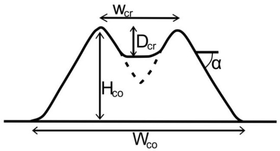
Figure 1.
Relationships between volcanic parameters. Wcr = crater width, Dcr = crater depth, Hco = cone height, Wco = basal width of cone, α = maximum slope angle (based on [2]).
One of the earliest studies was Colton’s [17] classic account of scoria cone morphology in the San Francisco Volcanic Field, Arizona. He classified them into five degradation stages of cones and basaltic flows on the basis of weathering. Scott and Trask [18] studied the morphologic, morphometric, chemical, and radiometric data of scoria cones and lava flows in the Lunar Crater volcanic field, Nevada: using maximum cone slope and cone width/cone height ratio, they derived relative morphologic ages for 15 cones. Settle [19] examined parameters of six volcanic areas (Mauna Kea (Hawaii), Mount Etna (Italy), Kilimanjaro (Tanzania), San Francisco Volcanic Field (Arizona), Paricutín (Mexico), Nunivak Island (Alaska)), including average volume, cone height and diameter. One of the most significant works in scoria cone morphometry came from Wood ([3,4]) who considered cones of the San Francisco Volcanic Field, which had been categorized by Colton [17] and Moore and Wolfe [20] into age groups. Wood examined and compared these and observed trends that were also found in five other scoria cone fields (Lunar Crater Volcanic Field (Nevada), Newberry volcano (Oregon), Wu-ta-lien-chi volcano (Manchuria), Etna (Italy), and Piton de la Fournaise (Réunion)) to determine if the degradation values are common to other scoria cone areas on Earth. Wood noted that (geological) maps did not provide adequate information for sufficient resolution of certain parameters (e.g., crater diameter). He claimed that the cone height (Hco), height-to-diameter (Wco) ratio, and slope angles (α) decrease over time, while the ratio of crater diameter (Wcr) to cone diameter (Wco) (Figure 1) does not change with decay. Following Wood, a comparative morphometric study along with computer modeling was done by Hooper and Sheridan [21]. Surface erosion processes were modeled on an ideal scoria cone. Maximum slope values were calculated from field surveys, aerial photographs, and distance from contour lines. Digital terrain models (DTM) from the United States Geological Survey were used to supplement these data. Their modeling was based on the parameters described earlier: height, height to diameter ratio (Hco/Wco), crater depth to crater diameter ratio (Hcr/Wcr), and cone slope angle. According to these authors, the basis of relative age determination with comparative morphology is the study of morphological parameters that continuously decrease over time.
From the early 2000s, DTMs began to be increasingly used in morphometric studies, as they became more widely available with progressively better resolution. The correlations published in previous studies are mainly idealized for regular, circular, or elliptical cones. In the case of irregular cones, it is of great importance how the diameter is designated: Favalli et al. [22] examined the parameter changes due to lava flow inundation in scoria cone fields, and also the effects of emplacement on a (larger) volcano flank. Similar results were described by Fornaciai et al. [6]. Different resolution DTMs were used in 21 volcanic areas to compare different tectonic settings and climates. They stated that DTM resolution is crucial when selecting scoria cone areas. The 90-m SRTM (Shuttle Radar Topography Mission) is mostly inappropriate, the 30-m ASTER (Advanced Spaceborne Thermal Emission and Reflection Radiometer) can be useful, but only better resolution data are really recommended for scoria cone studies (e.g., 5 or 10 m-resolution LiDAR). Morphometric parameters (V, slope, Hco, Wco, and Wcr) and geometric ratios (Hco/Wco and Wcr/Wco) were calculated for a total of 542 cones.
2. Materials and Methods
2.1. Data Used
2.1.1. Chaîne des Puys Setting
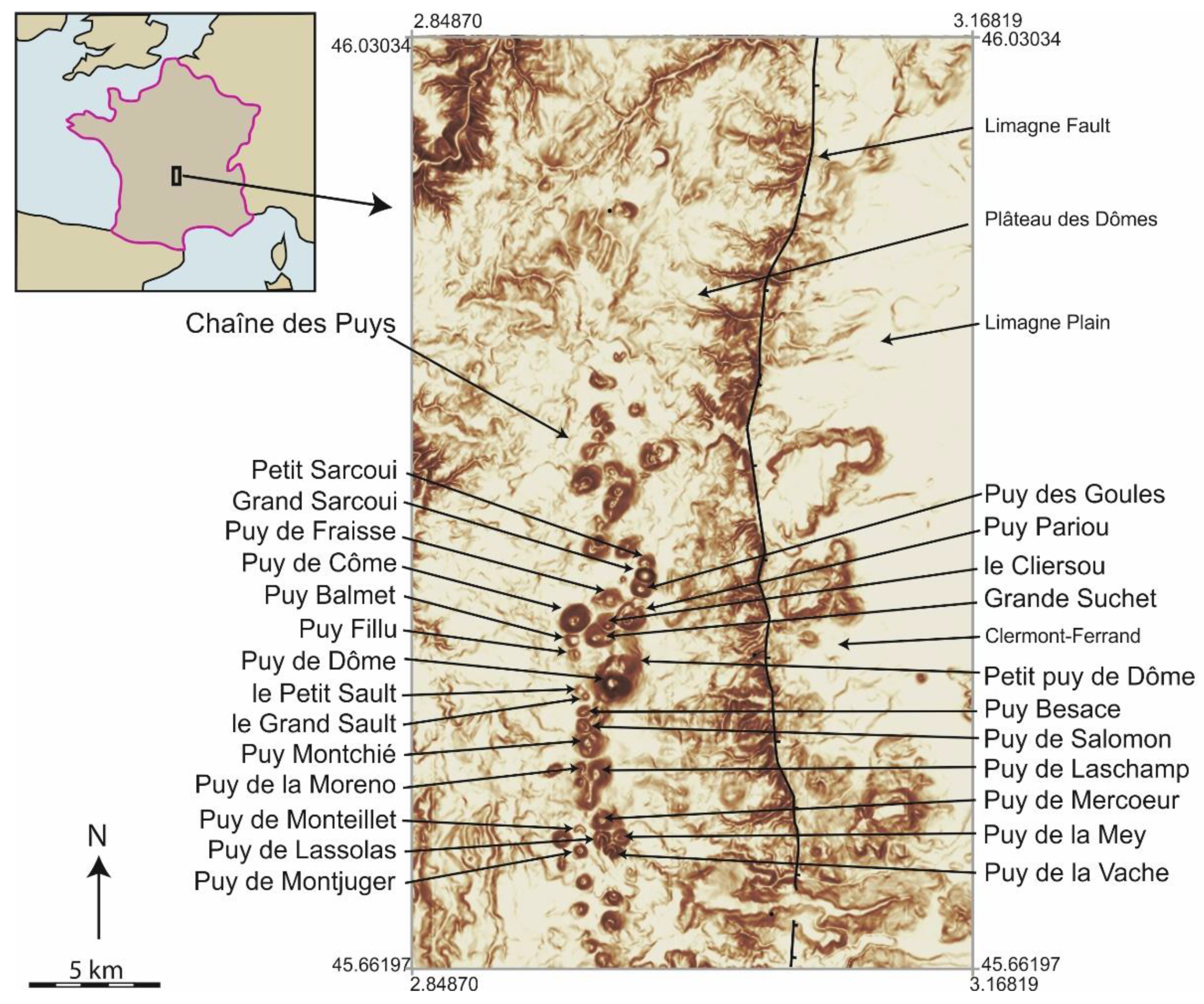
The study area here is the Chaîne des Puys, Auvergne, France (Figure 2). This is a compact alignment of more than 80 monogenetic volcanoes, long renowned for their diversity and variability [23,24,25]. The volcanoes are now part of a UNESCO World Heritage site [26]. The cones vary from simple basaltic cones to evolved trachyte domes and have a full range of volcano-geomorphic features such as small to large craters, breached craters, 10s m to 100s m-high cones, and complex flank geometries reflecting short but complex eruptions. We have taken 25 cones (Table 1), which are mostly true scoria cones. Some trachyte domes are included (Grand Sarcoui, le Cliersou, Puy de Dôme and Petit puy de Dôme, see in Table 1) to explore their similar, but subtly distinct morphometries. The cones and domes share similar construction characteristics, in that they are both formed by accumulation of fragmented material on slopes. The difference is that cone slopes are formed of scoria thrown out by explosions, while dome slopes by the crumbling of lava extruded at the summit. The resulting slopes appear very morphometrically similar because of this parallel evolution [27]. The present geological map of the Chaîne des Puys has been developed progressively since 1975 [28] and provides a classification of the cones into their different compositions and ages that are used in this study [24].
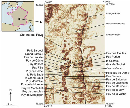
Figure 2.
Slope map of the Chaîne des Puys volcanic field and its surrounding (regional 10 m CRAIG DTM, modified from [30]) for identification of the cones (see the IDs in Table 1).

Table 1.
Summary of the geology, the ages [24] and the calculated classic morphometric parameters of the scoria cones and lava domes of Chaîne des Puys.
Studies on the Lemptégy volcano and associated cones [29,30,31] have shown the complex interplay between eruptions and the volcano’s surface morphology. Thus, that area provides a full set of scoria cone types that have also been closely researched for their constructional processes.
2.1.2. LiDAR DTM
The selection of DTM (or previously DTM) for morphometric studies is always a key issue. In most of the cases, the experimenter has a limited choice in terms of resolution and accuracy. Lower resolution DTMs underestimate the slope angles; therefore, it is advisable to use higher resolution data if available. However, previously, a common opinion was that, in case of scoria cones, being mostly regular in shape, this difference is not crucial, as the slopes of the cones are rather uniform (this can be disproved, e.g., [32]). Unfortunately, this is not the case, because the irregularities modify the slope distribution introducing a bias. Even if the man-made structures are present in the data, LiDAR DTMs are a better approximation of the ground surface than that of stereophotogrammetry-based data.
This is the reason we opted to use the LiDAR data for our studies. The Chaîne des Puys not only provides an exemplary area to study scoria cone morphometry but is covered extensively by LIDAR (CRAIG: Centre Regional de Informational Geographique—[33]). Two data sets are of particular value, LIDARVEGNE [34], a 0.5 m resolution covering of the central part of the chain, and LIDARCLERMONT [34], a 5 m-spacing general LIDAR data set made to cover the Clermont Auvergne Metropolitan area. All of the LIDAR is open data, and available from CRAIG. These data have been properly processed, and, even if there are man-made structures (roads, some buildings) present in the data, the overall extent of these non-geomorphic features is negligible in the area of the scoria cones.
2.2. Methods
2.2.1. Classic Morphometry
Based on the original methodology described by Settle [19], cone height was defined as the difference between the maximum value of the crater rim, or the summit elevation and the average basal elevation. Cone width or basal diameter (Wco) was calculated as the average of the maximum and the minimum diameters of each cone. These calculation methods were used by other researchers, e.g., [3,4,21,22,35,36]. Crater width or diameter (Wcr) was defined as the average of the maximum and minimum diameters of each crater. Crater depth (Dcr) is the difference between maximum rim or summit elevation and the lowest elevation in the crater. The usefulness of the slope angle (and deriving relative cone ages from it) were identified [18]. Before the appearance of digital terrain models, slope angles were measured in the field, taken from photographs [37] or determined with the help of the contour lines of topographic maps [3,4]. Over time, as the edifice is eroded, it is expected that both the maximum and average slope values decrease: the cone becomes smaller and smoother, as the erodible materials from the higher regions are either transported to the base of the cone (under dry climates) or further away (humid climates). As a result, the maximum slope angle would become smaller than that of the initial cone. Hasenaka and Carmichael (here after referred to as H&C) [35] defined how the average slope angle (which is another indicator of changing morphology) can be calculated, depending on whether a cone has or has no crater. For cones which still have a crater, the average cone slope angle (Save) is defined by:
where Hco is cone height, Wco is cone width or diameter, and Wcr is crater width or diameter. For cones that have lost the crater to erosion or did not have one originally (Wcr = 0), the average slope angle can be calculated by:
Save = tan−1[2Hco/(Wco − Wcr)],
Save = tan−1[2Hco/Wco]
2.2.2. Sectorization
Based on the previous literature presented above, we see that generally the whole cone has been used for morphometry. This method greatly simplifies the calculations because the cone can be characterized by only a few numerical values. However, the variability of the cone (e.g., asymmetry) is not reflected. To explore this, the method of sectorization has been introduced ([38] and this paper). Sectorization is easiest to understand for circular symmetric cones. The sectors are selected in the radial direction using the following main steps (Figure 3):
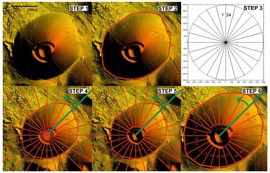
Figure 3.
Example of the sectorization steps described in the text. The green line (Steps 4–6) indicates the selected primary direction and the whole setting is rotated to the 12 o’clock position indicated by the green arrow (LiDAR DTM with shaded topography).
- 1.
- determine the center of the scoria cone,
- 2.
- determine the outline of the scoria cone,
- 3.
- create the initial (basal) sectors,
- 4.
- shift/rotate the starting sectors,
- 5.
- determine the crater rim,
- 6.
- create the final sectors.
Steps #1 and #2 are de facto standard steps, which should be performed not only for sectorization, but also for any morphometric analysis of scoria cones. Nowadays, these steps are (mostly) based on digital terrain models, ideally correlated with geological maps. The base of the cone was defined as the concave break in slope between the cone slope and the surrounding terrain (e.g., as in Figure 1). In many cases, this was the low slope plateau, and, in others, a sharp slope change between one cone and the adjacent one (see Figure 3, Steps 1 and 2). However, the best and most realistic result can be achieved by supplementing these with field data collection. Therefore, each cone base was manually drawn and checked by several users to verify the results.
Step #3: the starting sectors had to be adjusted to scoria cone sizes: we created a starting circle with a radius large enough to fit the largest scoria cone of the area. In this case, we created a maximum radius of 3000 m. Choosing the (angular) size of the sectors is also an important step: if it is too large (e.g., the central angle is 45°), the smaller surface changes will not modify the sectorial values—in the same way as if we consider the cone as a whole. If it is too small (too detailed, like 4°), then the larger correlations cannot be detected because small changes can considerably influence the sector value. As a compromise solution, the sectors were created in every 15° angle, so the entire circle was covered by 24 sectors. The sectors were numbered counterclockwise, sector number one is located at 12 o’clock. Thus, the whole circle has been split into twenty-four angular sectors, with (relative) central coordinates of (0, 0). These abstract sectors will henceforth work as ‘cookie cutter’ shapes in the next steps.
Step #4: the sectorial shapes created in Step #3 are used as follows: (0, 0) centered shapes are shifted to the center (Step #1) of the selected scoria cone. In some cases, we also changed the direction of sector number one (so not at 12 o’clock) by rotating the pattern. If the crater is not intact, but has collapsed or disappeared due to degradation, or there is any other morphological feature that distorts the circular symmetry, the centerline was rotated to the possible axis of symmetry. The starting direction was also rotated if the shape of the scoria cone was elongated in any direction. The main direction was chosen by the direction of the major axis. At the end of this task, the 24 sectors have a corresponding real-coordinate center, and the starting direction is also selected.
Step #5: the optional presence of a crater plays a significant role in the calculations: the slope values are greatly influenced by the crater, but the appearance/shape of the cone is less prominent, so it is advisable to omit the crater from the sectorial calculations. In the case of an ideal, circular cone, a doughnut-shaped mask is applied to the DTM: the middle part covered by the crater is omitted. To do this, the detection of the crater rim has to be done at first and then a (concentric) circle is fitted to it. Starting from the center, the farthest point of the crater rim was found radially, and this distance became the radius of the circle to be cut out. After the "cut-out," each sector can be described by four coordinate pairs of a trapezoid.
Step #6: the final resulting shapes are obtained as the intersection of the sectors formed in Step #5 and the shape bounded by the outlines created in Step #2.
3. Results
3.1. Results of the Classic Morphometry Parameters
Porter [2] selected a group of 30 Mauna Kea cinder cones and reported an empirical relationship of Hco = 0.18 Wco. Bloomfield [39] did the same for 41 cones within a section of the Mexican Volcanic Belt to the east of Paricutín. A mean cone height/width ratio for Holocene cones of 0.21, and a mean Hco/Wco of 0.19 for well-formed and relatively young Pleistocene cones was obtained. Settle [19] used a Hco = 0.2 Wco reference line that characterizes the initial shape of cinder cones formed in both types of volcanic provinces prior to erosive degradation. For our initial work, we made this calculation too.
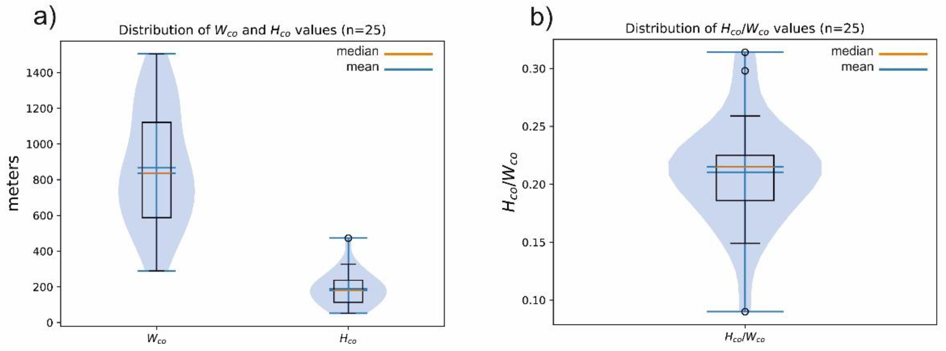
Scoria cone average diameters range from 290 m to ~1500 m with a mean of ~870 m and a median of 830 m. Average cone heights from ~50 m to ~470 m have a mean value of 190 m and a median 180 m (Table 1). Cones number 3, 8, 14, 27, and 28 do not have a crater.
The distributions of the Wco and Hco values are plotted in Figure 4a. The median (yellow) and mean values (blue) do not differ much; however, Wco values slightly, and Hco values are considerably positively skewed (skewness(Wco) = 0.26; skewness(Hco) = 0.99).
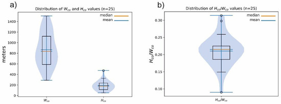
Figure 4.
(a) Distribution of the basal diameter (Wco) and the height of the cone (Hco) and (b) distribution of the Hco/Wco values of the studied 25 volcanic cones of the Chaîne des Puys.
Similar to other authors (e.g., [2,4,19,21]), we also considered the relationship of the basal diameter and the height of the cone via Hco/Wco values, and we also analyzed this relationship. The distribution of the Hco/Wco values is plotted in Figure 4b. The distribution of these ratio values does not show skewness (=−0.146) and the mean (=0.21) and the median (=0.215) values are very close to each other. It also shows a great similarity to the values used by aforementioned authors (0.18, 0.19, 0.21).
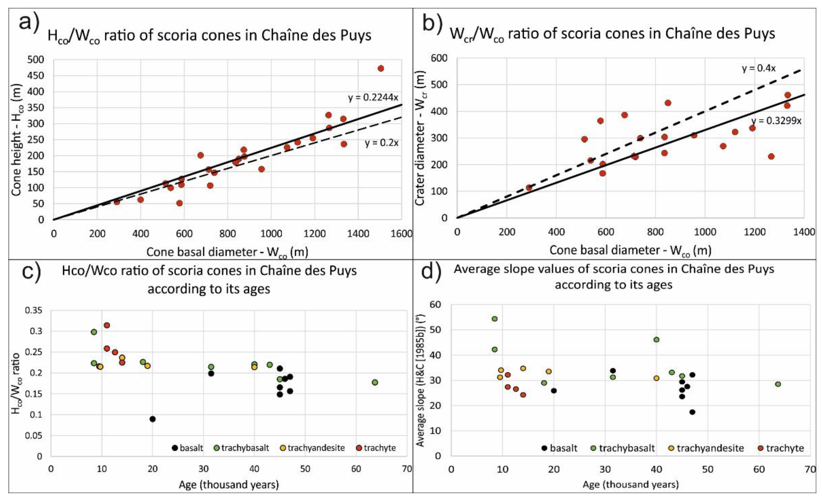
We emphasize that each of the calculations listed and defined above describes a symmetric cone (with or without a crater). If we consider these single-value descriptors of the geometry, the distributions of the related values of Chaîne des Puys follow this trend. Cone height (Hco) versus cone basal diameter (Wco) is plotted in Figure 5a (number of cones = 25): the dashed line represents Settle’s Hco = 0.2 Wco, the solid line represents our data’s calculated trendline Hco = 0.2244 Wco. In Figure 5b, the Wcr/Wco ratio for n = 20 cones can be seen. A reference (dashed line) is that of Porter’s Wcr = 0.40 Wco and is plotted for comparison.
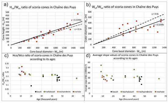
Figure 5.
(a) Hco/Wco ratio, (b) Wcr/Wco ratio, (c) Hco/Wco ratio according to ages (black: basalt, green: trachybasalt, yellow: trachyandesite, red: trachyte), (d) average slope values according to ages (black: basalt, green: trachybasalt, yellow: trachyandesite, red: trachyte).
According to Dohrenwend et al. [40] and Hooper and Sheridan [21], the measured values of the various morphometric parameters have an uncertainty of ±10% to ±15%. Our results also show similar scatter.
In Figure 5c,d, the Hco/Wco ratio and the average slope (Equations (1) and (2)) are plotted according to scoria cone age colored by lithology. In both cases, the trachytic cones/domes (red points) are situated in a compact group: these are some of the youngest landforms and have high Hco/Wco ratio. Basaltic cones are characterized by lower values; most of them are below 0.2 and 30°—separated from the trachyandesitic cones and roughly separated from the trachybasalts. In a few cases, the calculation method defined by Hasenaka and Carmichael [35] results in unexpectedly high average slope angles (even above 50°). These values far exceed the values published in previous research (e.g., [21]). These values likely resulted because, in the case of cones where the crater rim is not intact, one of the two crater diameter values (minimum/maximum) is missing, so no average value could be calculated.
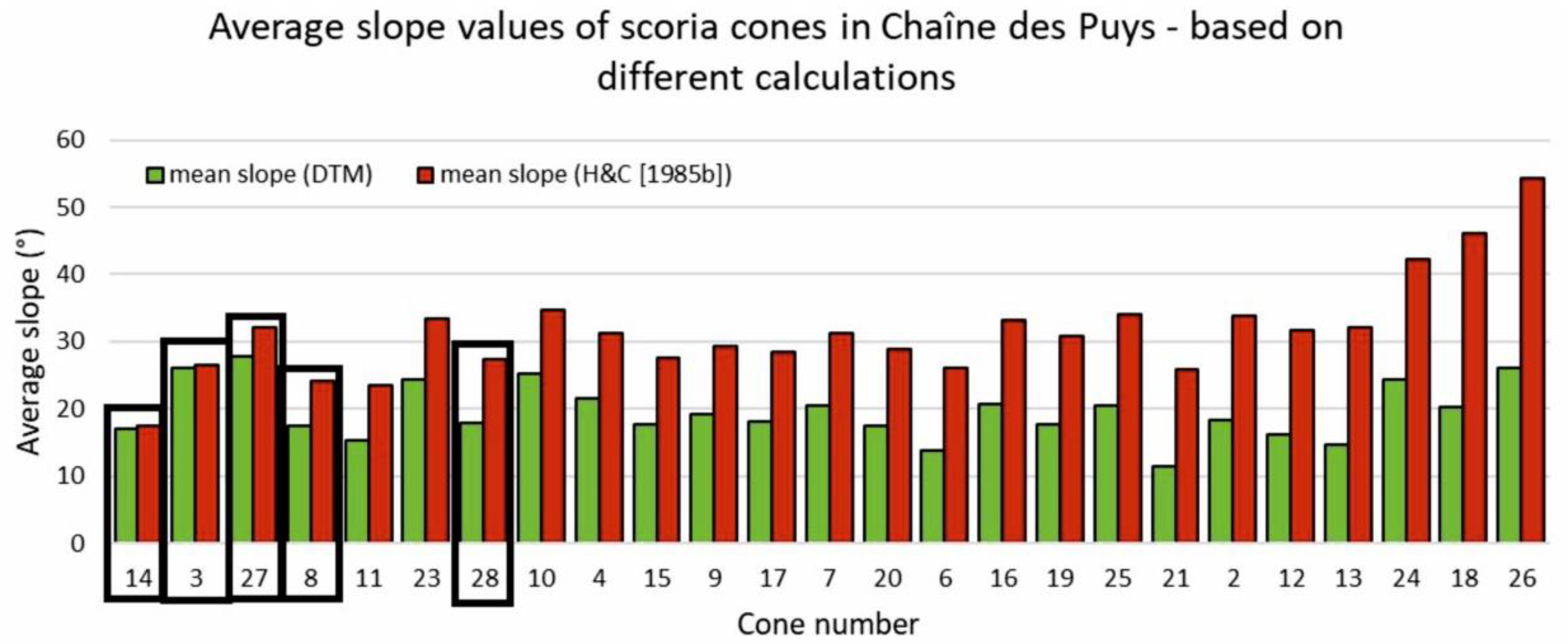
As was emphasized earlier, most previous authors considered single descriptors because they did not have access to adequate input data. The advantage of a digital terrain model-based morphometric research is that it is not necessary to use approximate or single values, but the terrain model can be used to easily obtain values closer to reality (depending on the resolution). Utilizing this advantage, we examined the average slope values of the scoria cones. In addition (following H&C [35]), we separated cones with craters as well. The sectorization method that we introduced requires the removal of the craters anyway (see Section 2.2.2), so we examined the mean slope angles in both cases—that is, either when calculating the entire cone (including the crater) or when we excluded the crater. In the case of the whole cone, the average slope angle is 19.62° ± 4.18°, while, without a crater, 19.57° ± 3.96°. The average difference between the two groups is 0.04° ± 0.8°.
In Figure 6, two average slope values are plotted. Red columns represent the mean slope calculated using the H&C [35] equations and green columns represent mean slope derived from the DTM (whole cone values). The order of the scoria cones is as follows: we examined the results obtained with the two types of calculations and arranged them in ascending order according to their differences. Cones framed in black are those that do not have a crater (four of them are domes): we can see that the difference between them is the smallest. Mean slope values calculated using the equations of H&C [35] are higher than values derived from DTM: in some cases, these are unrealistically high values. This overestimation has important implications: if we use the more realistic average slopes, the age/slope relationship seems to be more reliable (see 4. Discussion).

Figure 6.
Difference in average slope calculations: according to H&C [35] (red) and based on DTM (green). The former (parameter-based) method obviously overestimates the average slopes, sometimes extremely.
Following Hooper and Sheridan [21], Mann–Whitney tests were performed to compare the parameter distributions between four groups with different lithologies (Figure 5c,d, also see Table 1). Using a significance level of α = 0.05, the statistical tests were done for the four groups comparing age, Hco/Wco and mean slope angle (DTM) (Figure 7). For Hco/Wco, the basaltic, trachybasaltic, trachyandesitic, and trachytic group display progressively higher values, to some extent correlating with progressively younger ages, whereas, for mean slope, this relationship is less pronounced, and only the basaltic cones (being less steep) can be distinguished from the latter three lithological groups, which show higher but overlapping slope values. The Hco/Wco, values also significantly separate the trachyte from the trachyandesite lithologies, and, according to the average slope, the basaltic group is separated from the trachybasaltic one.
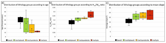
Figure 7.
Distribution of lithology groups according to (a) ages, (b) Hco/Wco, and (c) mean slope (black: basalt, green: trachybasalt, yellow: trachyandesite, red: trachyte).
3.2. Results of Sectorization Calculations
For the sectorization division, minimum, maximum, mean, median, and mode values were calculated for each sector (24) of the 25 examined cones. There are two cones that have been so destroyed (either by volcanogenic processes or post-eruptional erosion) that certain sectors are missing (cones 2 and 26). As was explained in Section 2.2.2, the starting (main) direction of the sectors was influenced by the shape of the cone. The other dominant direction is perpendicular to this main direction. These two imaginary lines gave the smallest and largest diameters of the scoria cone in most cases (used in Results), and they split the whole cone into quarters. With these quarters, the cone can be well characterized in terms of symmetry (see later). In Figure 8, the histograms of the median slope angles are plotted.
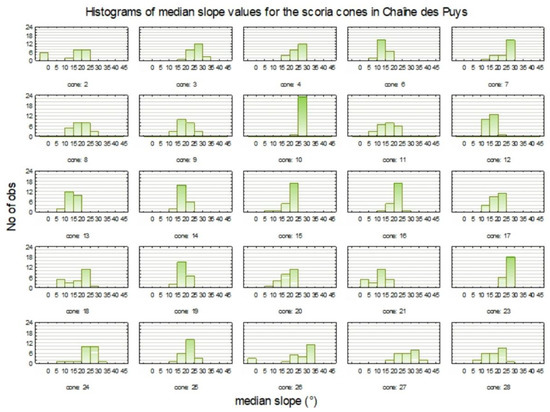
Figure 8.
The histograms of the median slope angles of the sectors for the 25 cones studied of the Chaîne des Puys.
Theoretically, a perfectly regular cone would have a single slope value for all sectors; in other words, the histogram would show a single, sharp peak. Consequently, the fewer bins that are filled with values, the more regular, rotationally symmetric is the cone. For instance, Cone 10 has only median slope values between 25° and 30° in the sectors. This cone is really close to regular, even if it is somewhat elongated.
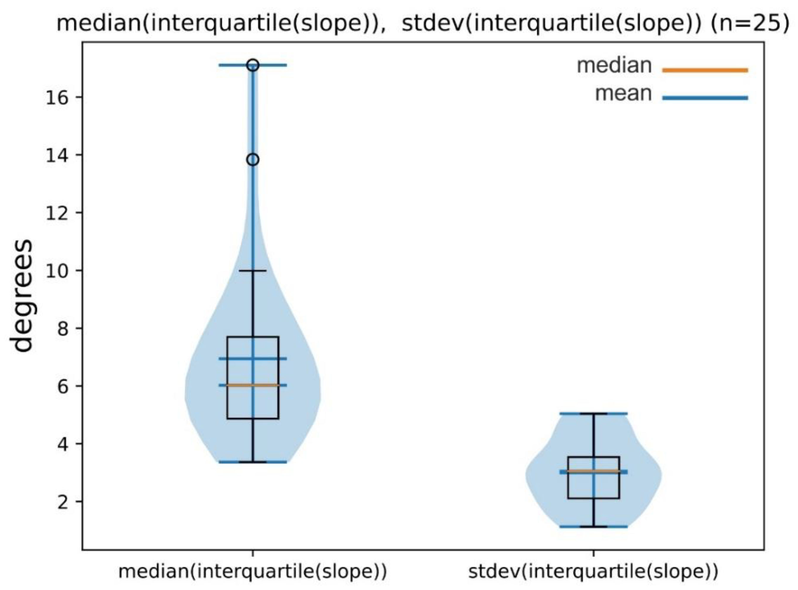
It is quite straightforward to study the interquartile values (differences of the values at 75% and 25% of the distribution) to assess how compact the distributions are. As many authors assumed that the slope distribution is typically rather peaked because of the apparent symmetry of the cones, we found it informative to present the interquartile distributions of the slopes (whole cone) for the studied individual edifices. In the case of highly regular cones, the median values of interquartile range should be relatively low (all sectors should be similar), and the standard deviation of the interquartile ranges should be close to zero (all distributions of the sectors should be similar). Figure 9 shows the results for the studied cones.

Figure 9.
Left: the median values of the interquartile ranges of the sectorial slope distributions for the 25 cones studied of the Chaîne des Puys; right: the standard deviations of the same.
However, it is important to clarify that the slope angle distribution is a statistical result, independent from the spatial (directional) contexts; thus, it does not give an accurate picture of the overall symmetry of the cones. To quantify the symmetry/asymmetry of the cones, the slopes of sectorized parts have been further evaluated. Most of the findings are discussed in the next section in the context of the lithology and age of the cone.
4. Discussion
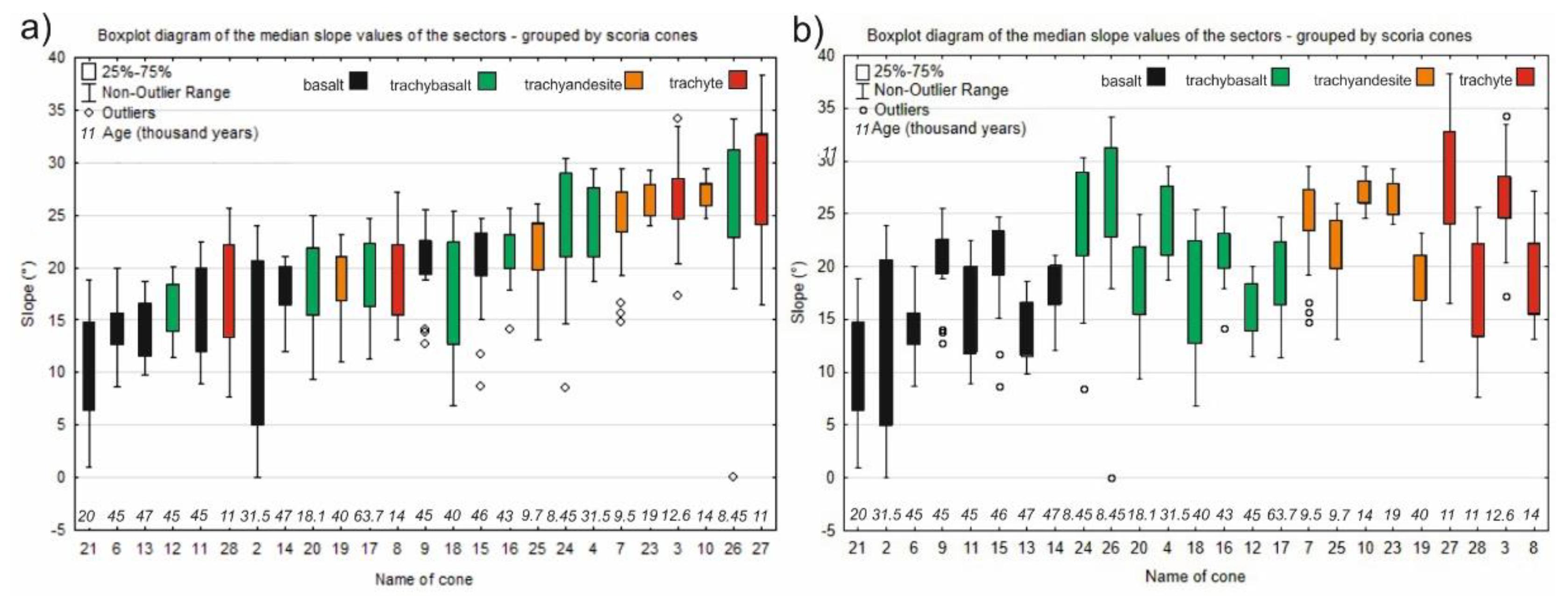
In Figure 10a,b, boxplot diagrams of the median slope values of the sectors can be seen, supplemented with information on lithology and age. In Figure 10a, the cones were plotted according to increasing median values. The figure suggests the same conclusion that we can draw from Figure 7c: the slope values are constrained by the lithological characteristics rather than by age. In order to emphasize this conclusion in Figure 10b, the cones were grouped by the lithology and then, within the groups, arranged according to their age.
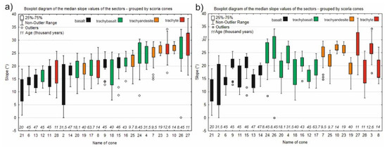
Figure 10.
Boxplot diagrams of the median slope values of the sectors. Cones plotted according to (a) increasing median values and (b) according to lithology and then ages (black: basalt, green: trachybasalt, yellow: trachyandesite, red: trachyte).
Figure 10b suggests that, for basaltic and trachytic cones, there no relationship with the age. In the case of trachyte, the ages are so close to each other that we cannot expect any correlation. In the case of basalt, there are two age groups: an older one of 45–47 ka, and a younger but more distributed group ranging from 20 ka to 31.5 ka. Concerning trachybasalt and trachyandesite cones, especially the latter ones, a decreasing trend can be observed. For trachybasalts, the regression line Hco/Wco = −0.0014 × age + 0.2669 (R2 = 0.5912) and Save = −0.117 × age + 24.404 (R2 = 0.4537) can be obtained. For trachyandesitic cones, the correlation is even weaker.
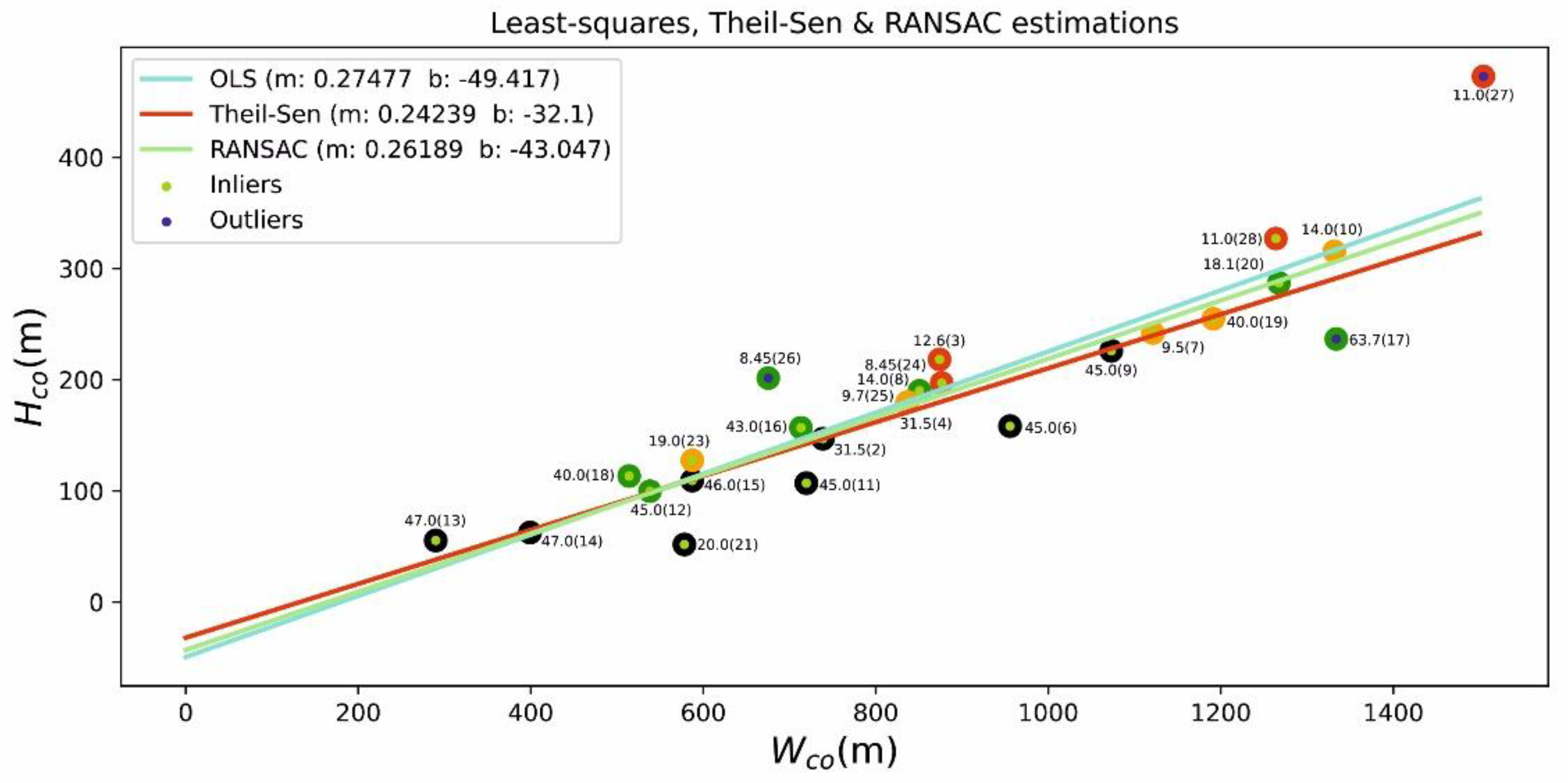
The distribution of points in Figure 5a,b indicates some heteroscedasticity, i.e., some points seem to follow a different trend. In order to study this, the Theil–Sen estimator [41,42] and RANSAC algorithm [43] have been applied to the data.
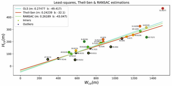
Figure 11.
Modeling of Wco–Hco relationship using the ordinary least squares method (OLS), Theil–Sen estimation and the RANSAC algorithm. The values indicated are the ages of the cones, and the IDs (see Table 1) are indicated in brackets. The color code is the same as for Figure 5, Figure 7 and Figure 10.
The three models (ordinary least squares (OLS), Theil–Sen estimator, and RANSAC algorithm) do not differ too much. However, it can be observed that robust models (Theil–Sen and RANSAC) gave more similar results. It is interesting to note that all trachytic cones/domes and two basaltic ones appear as outliers in the RANSAC model.
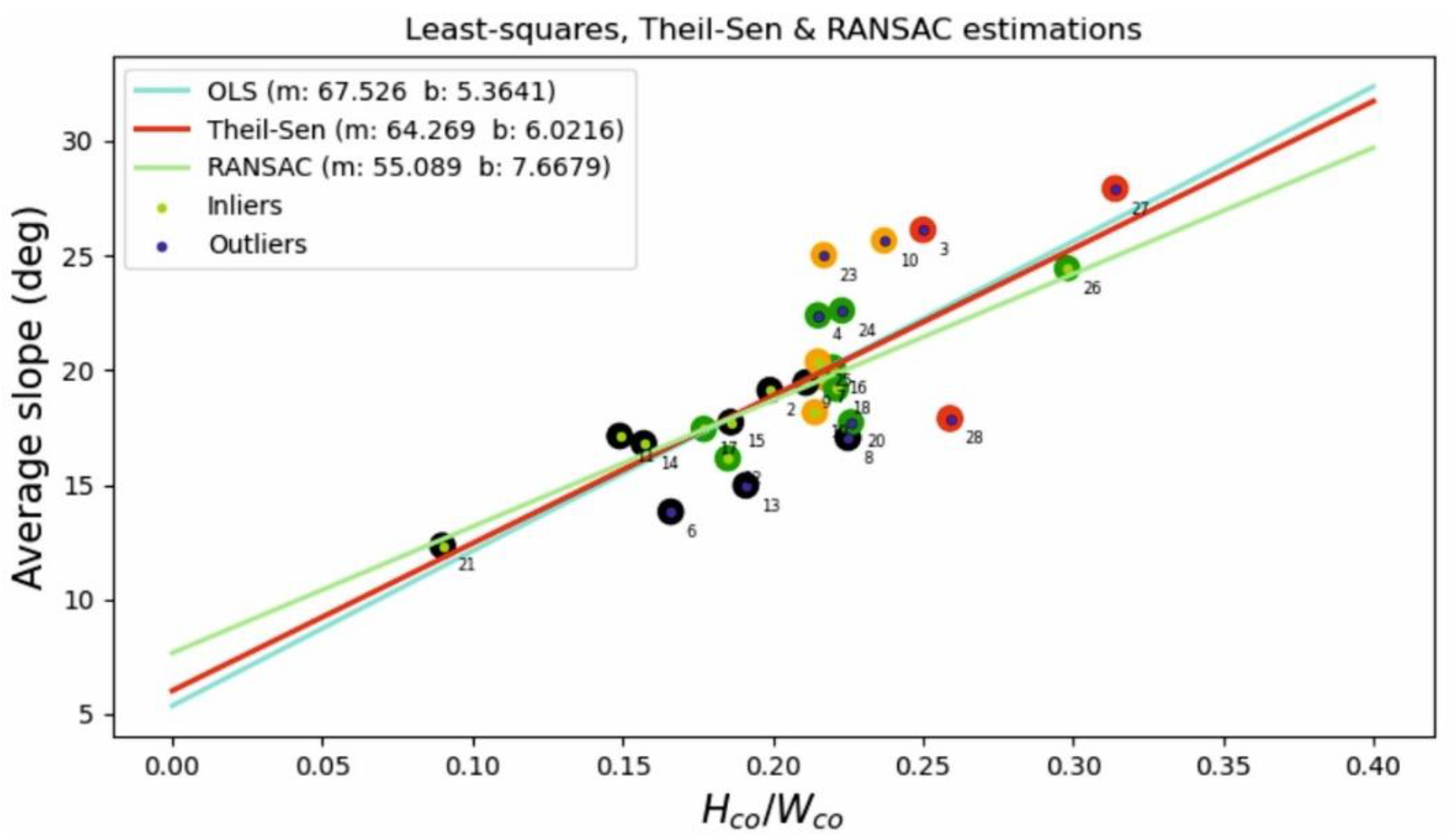
Although it is expected to describe the same phenomenon, analyzing the average slopes in the light of the Hco/Wco ratio, the heteroscedastic character is more obvious (Figure 12). This figure demonstrates a few interesting behaviors:

Figure 12.
Modeling of average slope Wco/Hco relationship using the ordinary least squares method (OLS), Theil–Sen estimation, and RANSAC algorithm. The values indicated are the IDs of the cones.
- In this case, the least squares and the Theil–Sen regression give similar results, whereas the RANSAC solution enhances the special behavior of some points too.
- The trachytic domes are well off any regression line; consequently, RANSAC identifies them as outliers in this relationship as well.
- The inliers of the RANSAC solution encompass six basaltic cones, a few trachybasaltic, and two trachyandesitic cones.
- Even if some of them are found to be outliers by RANSAC, trachybasaltic cones are mostly aligned with the trend. However, trachyandesitic cones form rather a compact group if they are considered separately.
- It is interesting to note that six basaltic cones (out of 8) are strongly aligned, indicating a stronger relationship.
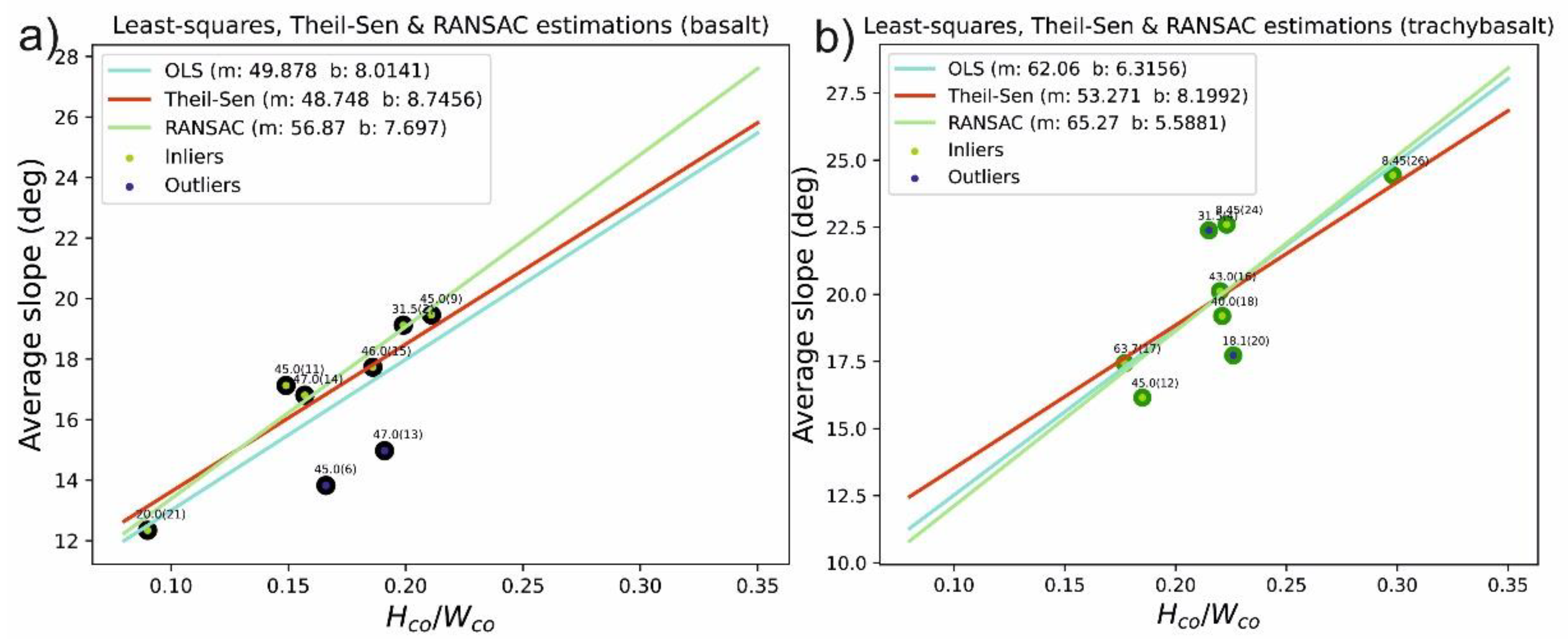
- The behavior of the basaltic cones motivated us to analyze them separately as well, in particular since this is the largest lithological group of eight cones. The result is presented in Figure 13a.
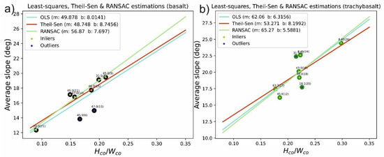 Figure 13. Modeling of average slope and Hco/Wco relationship of (a) basalt (b) trachybasalt cones using the ordinary least squares method (OLS), Theil–Sen estimation, and RANSAC algorithm. The values indicated are the ages of the cones, and the IDs (see Table 1) are indicated in brackets.
The six cones are aligned and dominate the whole group as expected: RANSAC identifies them as inliers, whereas two other basaltic cones are categorized as outliers. Figure 13a also indicates the ages of the cones. The age distribution does not follow a regular trend. We also tested the same selection for trachybasaltic cones (Figure 13b); in this case, the relationship is also questionable because of the appearance of several cones in the center.
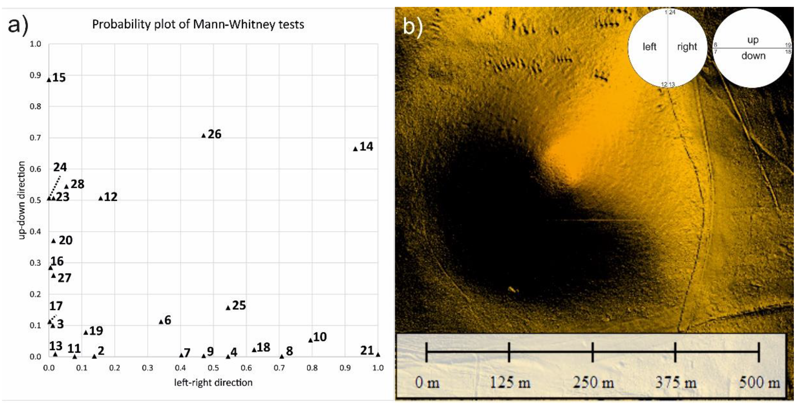
To examine the symmetry of the cones, the cones were analyzed along two symmetry axes (see the method above), and the different slope values obtained within the quarters were examined. The cones divided into 24 sectors were examined as follows: we first examined the difference between the median slope values in sectors 1–12 and 13–24 ("left-to-right") with the help of Mann–Whitney tests (significance level α = 0.05). Then, we examined the same values in a different grouping: 7-8-9-..16-17-18 and 19-20-21-..-4-5-6 ("up-down") as it is shown in the right above of Figure 14b.

Figure 14.
(a) probability plot of Mann-Whitney tests comparing the distributions of the left-right and up-down (forward backward) sectorial parts of each considered cones. The higher the value, the more symmetric the cone is in that directional sense; (b) cone 14, which is the most symmetric one according to the chart in the left panel. The definition of the two symmetry axes is right above.
We examined whether the "left-to-right" and "up-down" directions relative to the starting (main) direction are significantly different. Two p-values, pLR and pUD were obtained for each cone, which are plotted in Figure 14a.
The closer a cone is to one of the axes, the more asymmetrical it is in that respect. Cones with one p-value low and the other high (close to 1) elongated in some (denoting the high value axis) direction and are elliptical. An ideal, fully symmetrical cone of rotation would be in the (1.0, 1.0) position. In Figure 14b, Cone 14 is shown (LiDAR DTM with shaded topography). Both p-values of this cone are high (0.93 and 0.67), which means that they are symmetric, not only on the "left-to-right direction" and "up-down direction" separately, but also close to a regular cone.
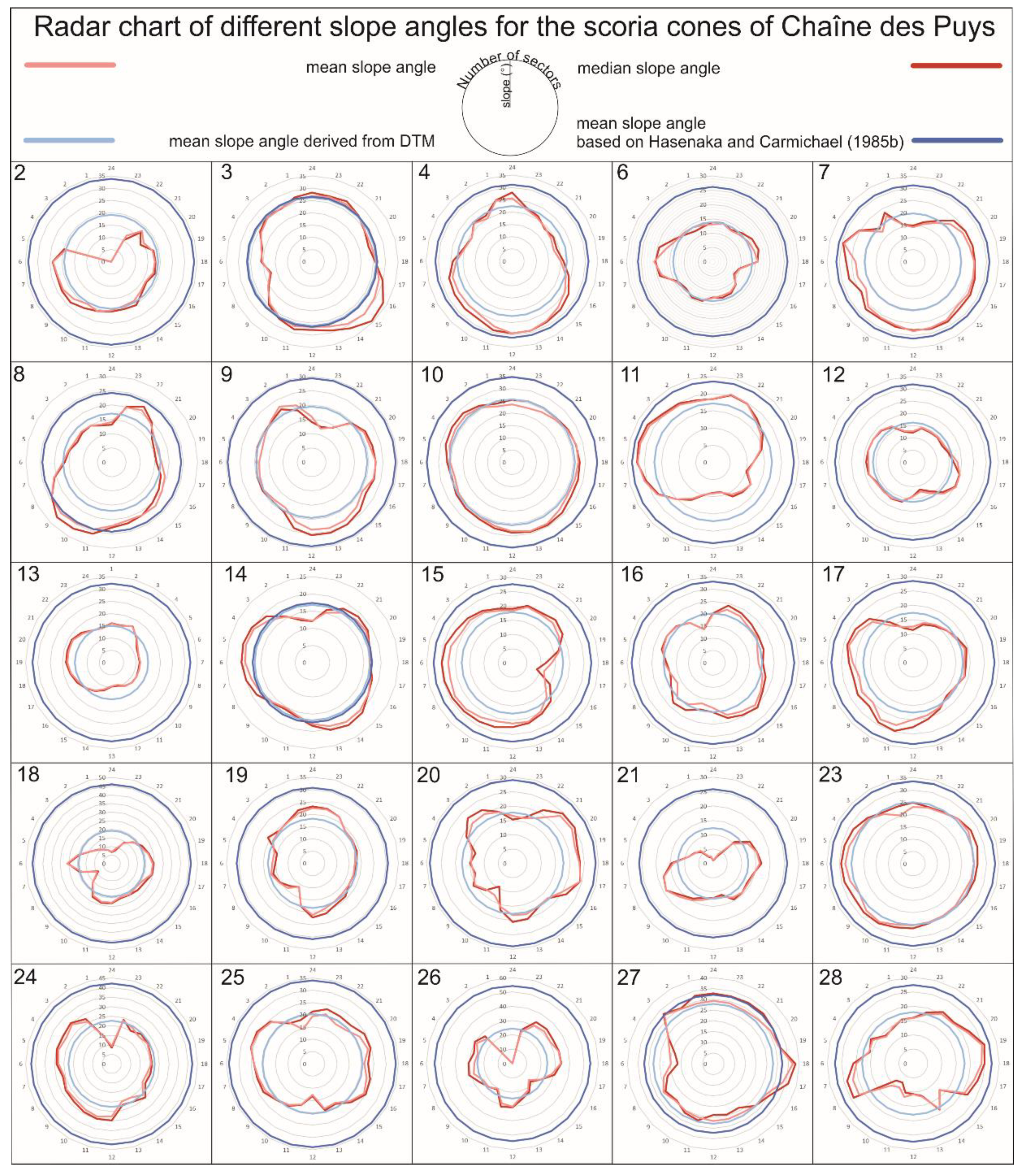
The important message of Figure 14b is that, in most of the cases, the symmetry of the slope distributions cannot be assumed along the hypothesised symmetry axes. This observation motivated us to visualize the two most important statistical values characterizing the sectors in the light of the classic parameters. In order to be able to compare the differently calculated slope angle values clearly and simply, we plotted them on radar charts (Figure 15). In the outermost circle, the sectors from 1 to 24 are indicated in a counterclockwise direction. The inner fainter circles show the slope values in 5-degree steps. Four types of values are displayed: two are bound to sectors (reddish), two to the entire cone (blueish). The sectorial data are the mean and median values of the slopes in the respective direction (within one sector). Since all sectors have the same value, the regular circles are indicating calculated mean slope (for the whole cone) and the result of mean slope calculated according to the method of Hasenaka and Carmichael [35]. In most cases, the latter shows a much larger value than those obtained by the other three calculations, except for cones without craters (see also above).
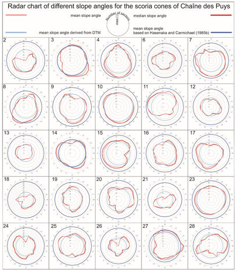
Figure 15.
Sectorial values of mean slope angles (light red), of median of the slope angles (red). Blue circles are calculated values for the entire cone: light blue is the DTM-based mean slope, whereas the blue (outer) one is calculated according to the method of Hasenaka and Carmichael [35]. Note the great variety of the sectorial values.
It is clear that, in most of the cases, the H&C [35] method overestimates all types of calculated slopes. On the other hand, naturally, the mean and median slopes are strongly related to the sectorial distribution. For the roughly regular cones, they are close to each other (e.g., Cone 10 and Cone 23). However, in the other way round, if we consider the symmetry of the curves, we will not necessarily find a circularly symmetric cone (e.g., Cone 12 or Cone 13).
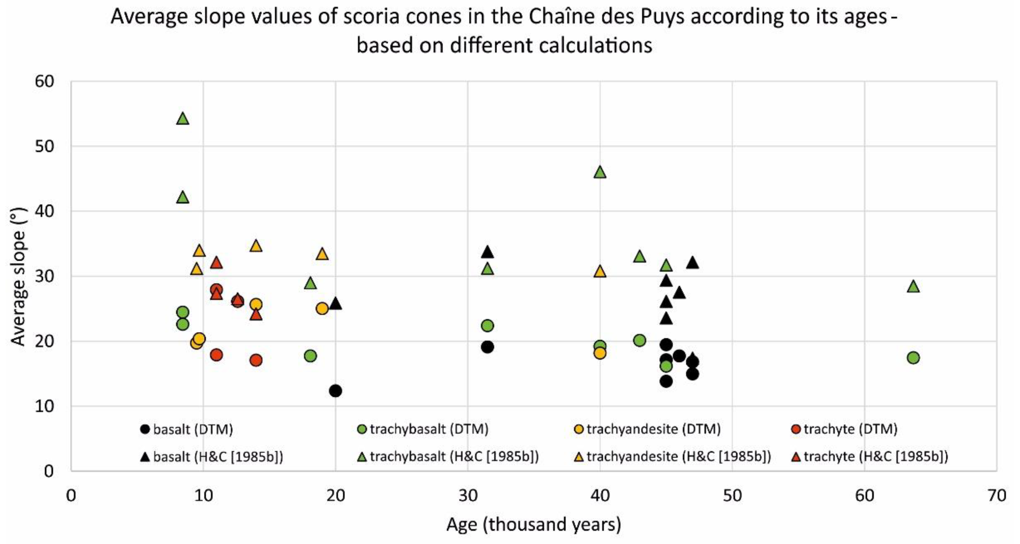
Last but not least, we consider the age–geometry relationship as well. Figure 16 summarizes the classic slope value calculation by Hasenaka and Carmichael [35], the slope distribution calculations of this paper, and the ages of the cones. Similarly to the previous observations, the figure suggests that DTM-based slope values give a more reliable picture about the cones, assuming a certain level of regularity.
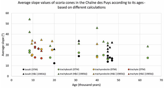
Figure 16.
Summary of slope values based on H&C equations [35] (dots) and DTMs (triangles) according to its ages. Coloring is based on lithology (black: basalt, green: trachybasalt, yellow: trachyandesite, red: trachyte).
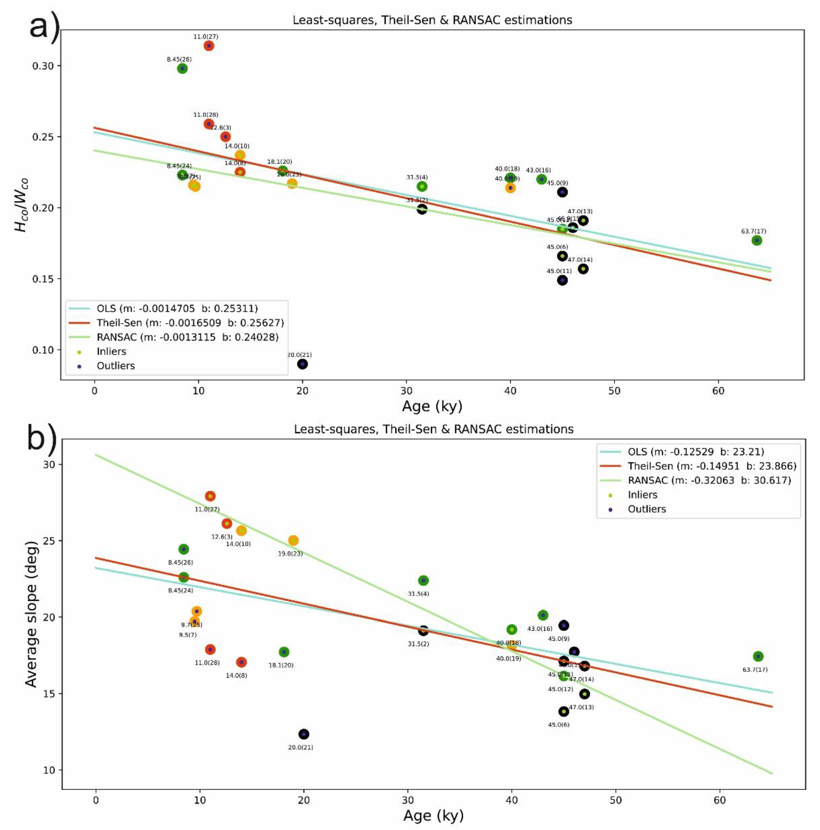
Finally, regression models have been calculated for the morphometric parameters and ages of the cones (Figure 17). Both the Hco/Wco and (DTM-based) average slope values show relatively large scattering in the figure showing a certain trend. The simplest linear models are very similar in the case of regression of Hco/Wco values. This is due to the age grouping of two typical age ranges: 10–14 ka and 40–47 ka. In this case, cones of various lithologies are in-line with the regression models.
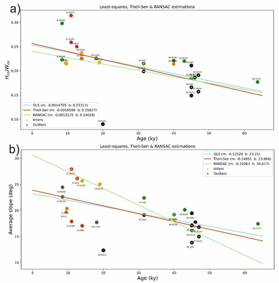
Figure 17.
(a) regression models for age vs. Hco/Wco ratio. All three models are similar with many outliers; (b) regression models for age vs. (DTM-based) average slope. RANSAC results in a completely different model, whereas the results of ordinary least squares fit and Theil–Sen estimator are similar.
Considering the (DTM-based) average slope angles (Figure 17), the situation is slightly different: ordinary least squares fit and Theil–Sen estimator practically result in being the same, whereas RANSAC finds a rather different model. Only a few cones are aligned with the former two models (mostly, but not exclusively basalts); RANSAC inliers are more numerous and all types of lithologies are represented in balanced numbers. Assuming limited validity to the regression models, either ca. 0.13 degrees/ky or 0.32 degrees/ky edifice destruction would be an estimate on destructional rates. Since these values have very high estimation error, at the current level of knowledge, they cannot be considered as of erosional origin. In order to get better models, further morphometric studies and more complex geomorphometric approaches are needed.
The Chaîne des Puys is a young volcanic field, compared with many studies, which range into millions of years, so it is likely that the degradational processes are more difficult to detect at such short time scales. In addition, as the cones are closely spaced, they tend to erupt material onto one another, and thus there is a possible constructional effect from material addition from nearby cones after an eruption is finished. This is something that may occur in all volcanic fields but would be most important where the cones are close, like in the Chaîne des Puys.
5. Conclusions
From the results of the morphometric analysis of the 25 cones studied of the Chaîne des Puys, the following conclusions can be drawn:
- The general assumption for scoria cones that the basal width (Wco) correlates with the height of the cone (Hco) could be verified. However, Hasenaka & Carmichael’s [35] calculation of average slopes overestimates the real slope values, sometimes to a great extent. We suggest that this method should be replaced by DTM-derived slope values, in agreement with a number of subsequent studies (e.g., [14]).
- In addition, a more detailed morphometric assessment that tackles the circular symmetry of the cones reveals that specific groups behave differently, and, in some cases, they define a separate trend or no trend can be detected. The slope distributions extracted from LiDAR digital terrain models indicate greater variability with lithology/composition than with age, at least over the age range of the volcanoes here.
- Nevertheless, within the same lithological group, subtle but possibly systematic trends can be detected for decreasing morphometric values (e.g., slope) with the age. Cones of different lithology/composition can have different relationships, and thus different composition cones produce slightly different shapes.
- Despite the attempt to characterize them separately, we can conclude that the time span of the trachytic cones/domes of Chaîne des Puys is too short for significant differences or correlations with the age to be detected with confidence.
- Morphometric sectorization resulted in separation into various types of symmetries. Some cones are close to a regular shape, but the majority of the cones are not circularly symmetric. These cones, however, often show other types of symmetry. The radar diagrams of specifically processed slope distributions show similarities and dissimilarities. These observations are encouraging to perform further statistical analysis of sectorial data that might reveal further relationships with tectonics, slope or wind directions.
- The initial aim to explore relationships of age and lithology with and morphometric parameters showed that lithology is a strong control, but only a faint age effect was detectable over the timespan of just under 100,000 years. The variability of original cone morphometry led to large errors in estimated rates. More detailed geomorphological approaches integrating lithological factors would be a next step, and applying the methods to a longer time span.
- The variability depicted in the morphometry is connected largely to the lithology and thus eruptive processes, and/or potentially with the angle of repose of various types of scoria. The methods here have the potential to explore such processes over a volcanic field. Further work is needed to understand all the diverse parameters, especially how different compositions produce different shapes, and how symmetry is connected to different factors.
Author Contributions
Conceptualization, B.S. and F.V.; methodology, B.S.; software, B.S. and F.V.; validation, B.v.W.d.V. and D.K.; investigation, ALL; resources, B.v.W.d.V.; writing—original draft preparation, ALL; writing—review and editing, B.v.W.d.V. and D.K.; visualization, F.V. and B.S. All authors have read and agreed to the published version of the manuscript.
Funding
This research received no external funding.
Institutional Review Board Statement
Not applicable.
Informed Consent Statement
Not applicable.
Data Availability Statement
The data presented in this study are available upon request from the corresponding author.
Acknowledgments
The authors are deeply indebted to the three anonymous reviewers whose constructive comments, linguistic, and structural suggestions considerably improved our manuscript. LIDAR DTM CRAIG open data site (www.craig.fr; accessed on 29 April 2021). For the statistical evaluations and visualization, various functions of the matplotlib and scikit-learn Python packages have been used, the authors’ work (e.g., Dan Nelson’s and Florian Wilhelm’s) is acknowledged.
Conflicts of Interest
The authors declare no conflict of interest. The funders had no role in the design of the study; in the collection, analyses, or interpretation of data; in the writing of the manuscript, or in the decision to publish the results.
References
- Karatson, D.; Yepes, J.; Favalli, M.; Rodríguez-Peces, M.J.; Fornaciai, A. Reconstructing eroded paleovolcanoes on Gran Canaria, Canary Islands, using advanced geomorphometry. Geomorphology 2016, 253, 123–134. [Google Scholar] [CrossRef]
- Porter, S.C. Distribution, Morphology, and Size Frequency of Cinder Cones on Mauna Kea Volcano, Hawaii. Geol. Soc. Am. Bull. 1972, 83. [Google Scholar] [CrossRef]
- Wood, C.A. Morphometric analysis of cinder cone degradation. J. Volcanol. Geotherm. Res. 1980, 8, 137–160. [Google Scholar] [CrossRef]
- Wood, C.A. Morphometric evolution of cinder cones. J. Volcanol. Geotherm. Res. 1980, 7, 387–413. [Google Scholar] [CrossRef]
- Walker, G.P.L. Basaltic volcanoes and volcanic systems. In Encyclopedia of Volcanoes; Sigurdsson, H., Ed.; Academic Press: Cambridge, UK, 2000; pp. 283–289. [Google Scholar]
- Fornaciai, A.; Favalli, M.; Karátson, D.; Tarquini, S.; Boschi, E. Morphometry of scoria cones, and their relation to geodynamic setting: A DEM-based analysis. J. Volcanol. Geotherm. Res. 2012, 217-218, 56–72. [Google Scholar] [CrossRef]
- Riedel, C.; Ernst, G.; Riley, M. Controls on the growth and geometry of pyroclastic constructs. J. Volcanol. Geotherm. Res. 2003, 127, 121–152. [Google Scholar] [CrossRef]
- de Silva, S.; Lindsay, J.M. Primary Volcanic Landforms. In The Encyclopedia of Volcanoes, 2nd ed.; Academic Press: Cambridge, UK, 2015; pp. 273–297. ISBN 9780123859389. [Google Scholar]
- Houghton, B.F.; Schmincke, H.-U. Rothenberg scoria cone, East Eifel: A complex Strombolian and phreatomagmatic volcano. Bull. Volcanol. 1989, 52, 28–48. [Google Scholar] [CrossRef]
- Calvari, S.; Pinkerton, H. Birth, growth and morphologic evolution of the ‘Laghetto’ cinder cone during the 2001 Etna eruption. J. Volcanol. Geotherm. Res. 2004, 132, 225–239. [Google Scholar] [CrossRef]
- Pioli, L.; Erlund, E.; Johnson, E.; Cashman, K.; Wallace, P.; Rosi, M.; Granados, H.D. Explosive dynamics of violent Strombolian eruptions: The eruption of Parícutin Volcano 1943–1952 (Mexico). Earth Planet. Sci. Lett. 2008, 271, 359–368. [Google Scholar] [CrossRef]
- Nemeth, K.; Kereszturi, G. Monogenetic volcanism: Personal views and discussion. Int. J. Earth Sci. 2015, 104, 2131–2146. [Google Scholar] [CrossRef]
- Németh, K. Monogenetic volcanic fields: Origin, sedimentary record, and relationship with polygenetic volcanism. In What Is A Volcano? Canon-Tapia, E., Szakacs, A., Eds.; Geological Society of America: Boulder, CO, USA, 2010; Volume 470, pp. 43–66. [Google Scholar]
- Kereszturi, G.; Németh, K. Monogenetic Basaltic Volcanoes: Genetic Classification, Growth, Geomorphology and Degradation. In Updates in Volcanology-New Advances in Understanding Volcanic Systems; Németh, K., Ed.; Intech Open: London, UK, 2012; Volume 1, pp. 3–88. [Google Scholar]
- Smith, I.E.M.; Németh, K. Source to surface model of monogenetic volcanism: A critical review. Geol. Soc. London. Spec. Publ. 2017, 446, 1–28. [Google Scholar] [CrossRef]
- Corazzato, C.; Tibaldi, A. Fracture control on type, morphology and distribution of parasitic volcanic cones: An example from Mt. Etna, Italy. J. Volcanol. Geotherm. Res. 2006, 158, 177–194. [Google Scholar] [CrossRef]
- Colton, S.H. The basaltic cinder cones and lava flows of the San Francisco Mountain volcanic field. Mus. North. Ariz. Bull. 1937, 10, 1–49. [Google Scholar]
- Scott, D.; Trask, N. Geology of the Lunar Crater volcanic field, Nye County, Nevada. Prof. Pap. 1971, 599, 22. [Google Scholar] [CrossRef]
- Settle, M. The structure and emplacement of cinder cone fields. Am. J. Sci. 1979, 279, 1089–1107. [Google Scholar] [CrossRef]
- Moore, R.B.; Wolfe, E. Geologic map of the east part of the San Francisco Volcanic Field, north-central Arizona, scale 1:50 000. USGS Misc. Investig. Ser. Map 1987. [Google Scholar] [CrossRef]
- Hooper, D.M.; Sheridan, M.F. Computer-simulation models of scoria cone degradation. J. Volcanol. Geotherm. Res. 1998, 83, 241–267. [Google Scholar] [CrossRef]
- Favalli, M.; Karátson, D.; Mazzarini, F.; Pareschi, M.T.; Boschi, E. Morphometry of scoria cones located on a volcano flank: A case study from Mt. Etna (Italy), based on high-resolution LiDAR data. J. Volcanol. Geotherm. Res. 2009, 186, 320–330. [Google Scholar] [CrossRef]
- van Wyk de Vries, B. Volcanoes of France. In Volcanoes of Europe; Jerram, D., Scarth, A., Tanguy, J.-C., Eds.; Dunedin Academic Press, Ltd.: Edinburgh, UK, 2017; p. 256. ISBN 13: 978-1780460420. [Google Scholar]
- Boivin, P.; Besson, J.C.; Briot, D.; Camus, G.; De Goër de Hervé, A.; Gourgaud, A.; Labazuy, P.; Langlois, E.; de Larouzière, F.D.; Livet, M.; et al. Volcanologie de la Chaîne des Puys, scale 1:25 000. 1 sheet. In Editions Du Parc Naturel Régional Des Volcans d’Auvergne, 5th ed.; IGN: San Francisco, CA, USA, 2017. [Google Scholar]
- Scrope, G.P. Considerations on Volcanos, the Probable Causes of Their Phenomena, the Laws Which Determine Their March, the Disposition of Their Products, and Their Connexion with the Present State and Past History of the Globe; Phillips, W., Ed.; Cambridge University Press: London, UK, 1825. [Google Scholar]
- Haut Lieu Tectonique Chaîne Des Puys-Faille De Limagne-UNESCO World Heritage Centre. Available online: http://whc.unesco.org/fr/list/1434 (accessed on 27 April 2021).
- Shields, J. The Morphometry of the Chaine des Puys; Université Blaise Pascal: Aubière, France, 2010. [Google Scholar]
- Camus, G.; Goer de Herve, A.; Kieffer, G.; Mergoil, J.; Vincent, P.M. Volcanologie de la Chaîne des Puys 1:25 000. Parc. Nat. Régional des Volcans D Auvergne Clermont Ferrand 1975. [Google Scholar]
- Delcamp, A.; Vries, B.V.W.D.; Stéphane, P.; Kervyn, M. Endogenous and exogenous growth of the monogenetic Lemptégy volcano, Chaîne des Puys, France. Geosphere 2014, 10, 998–1019. [Google Scholar] [CrossRef] [Green Version]
- Petronis, M.S.; Vries, B.V.W.D.; Garza, D. The Leaning Puy de Dôme (Auvergne, France) tilted by shallow intrusions. Volcanica 2019, 2, 161–186. [Google Scholar] [CrossRef]
- Vries, B.V.W.D.; Marquez, A.; Herrera, R.; Bruña, J.L.G.; Llanes, P.; Delcamp, A. Craters of elevation revisited: Forced-folds, bulging and uplift of volcanoes. Bull. Volcanol. 2014, 76, 875. [Google Scholar] [CrossRef]
- Vörös, F.; van Wyk de Vries, B.; Székely, B. Geomorphometric Descriptive Parameters of Scoria Cones from Different Dtms: A Resolution Invariance Study. In Proceedings of the 7th International Conference on Cartography and GIS, Sozopol, Bulgaria, 18–23 June 2018; pp. 603–612. [Google Scholar]
- Accueil|Craig. Available online: https://www.craig.fr/ (accessed on 29 April 2021).
- 2011_Site_Puy_De_Dome_Lidarverne-Fichiers-Drive Opendata Du Craig. Available online: https://drive.opendata.craig.fr/s/opendata?path=%2Flidar%2Fautres_zones%2F2011_site_puy_de_dome_lidarverne (accessed on 27 April 2021).
- Hasenaka, T.; Carmichael, I.S. The cinder cones of Michoacán—Guanajuato, central Mexico: Their age, volume and distribution, and magma discharge rate. J. Volcanol. Geotherm. Res. 1985, 25, 105–124. [Google Scholar] [CrossRef]
- Hasenaka, T.; Carmichael, I.S.E. A compilation of location, size, and geomorphological parameters of volcanoes of the Michoacan-Guanajuato Volcanic Field, Central Mexico. Geof. Int. 1985, 24, 577–607. [Google Scholar]
- Ray, R.G. Aerial photographs in geologic interpretation and mapping. Prof. Pap. 1960, 373. [Google Scholar] [CrossRef] [Green Version]
- Vörös, F.; Pál, M.; Vries, B.V.W.D.; Székely, B. Development of a New Type of Geodiversity System for the Scoria Cones of the Chaîne des Puys Based on Geomorphometric Studies. Geosciences 2021, 11, 58. [Google Scholar] [CrossRef]
- Bloomfield, K. A late-Quaternary monogenetic volcano field in central Mexico. Acta Diabetol. 1975, 64, 476–497. [Google Scholar] [CrossRef]
- Dohrenwend, J.C.; Wells, S.G.; Turrin, B.D. Degradation of Quaternary cinder cones in the Cima volcanic field, Mojave Desert, California. GSA Bull. 1986, 97, 421–427. [Google Scholar] [CrossRef]
- Theil, H. A Rank-Invariant Method of Linear and Polynomial Regression Analysis. In Henri Theil’s Contributions to Economics and Econometrics; Springer Science and Business Media LLC: Dordrecht, The Netherlands, 1992; Volume 53, pp. 345–381. [Google Scholar]
- Sen, P.K. Estimates of the regression coefficient based on Kendall’s Tau. J. Am. Stat. Assoc. 1968, 63, 1379–1389. [Google Scholar] [CrossRef]
- Fischler, M.A.; Bolles, R.C. Random Sample Paradigm for Model Consensus: Applications to Image Fitting with Analysis and Automated Cartography. Commun. ACM 1981, 24, 381–395. [Google Scholar] [CrossRef]


Publisher’s Note: MDPI stays neutral with regard to jurisdictional claims in published maps and institutional affiliations. |
© 2021 by the authors. Licensee MDPI, Basel, Switzerland. This article is an open access article distributed under the terms and conditions of the Creative Commons Attribution (CC BY) license (https://creativecommons.org/licenses/by/4.0/).