Abstract
Anthropogenic and natural disturbances can cause degradation of ecosystems, reducing their capacity to sustain biodiversity and provide ecosystem services. Understanding the extent of ecosystem degradation is critical for estimating risks to ecosystems, yet there are few existing methods to map degradation at the ecosystem scale and none using freely available satellite data for mangrove ecosystems. In this study, we developed a quantitative classification model of mangrove ecosystem degradation using freely available earth observation data. Crucially, a conceptual model of mangrove ecosystem degradation was established to identify suitable remote sensing variables that support the quantitative classification model, bridging the gap between satellite-derived variables and ecosystem degradation with explicit ecological links. We applied our degradation model to two case-studies, the mangroves of Rakhine State, Myanmar, which are severely threatened by anthropogenic disturbances, and Shark River within the Everglades National Park, USA, which is periodically disturbed by severe tropical storms. Our model suggested that 40% (597 km2) of the extent of mangroves in Rakhine showed evidence of degradation. In the Everglades, the model suggested that the extent of degraded mangrove forest increased from 5.1% to 97.4% following the Category 4 Hurricane Irma in 2017. Quantitative accuracy assessments indicated the model achieved overall accuracies of 77.6% and 79.1% for the Rakhine and the Everglades, respectively. We highlight that using an ecological conceptual model as the basis for building quantitative classification models to estimate the extent of ecosystem degradation ensures the ecological relevance of the classification models. Our developed method enables researchers to move beyond only mapping ecosystem distribution to condition and degradation as well. These results can help support ecosystem risk assessments, natural capital accounting, and restoration planning and provide quantitative estimates of ecosystem degradation for new global biodiversity targets.
1. Introduction
Ecosystem degradation is among the most important contributors to biodiversity loss [1]. Degradation is often broadly defined as a departure from an ecosystem’s natural range of variability [2] and can have substantial detrimental impacts on an ecosystems’ capacity to sustain services, such as carbon storage, resource provisioning, and water purification and regulation [3,4]. Such departures from natural variability thus lead to negative socioeconomic impacts at scales ranging from local to global [5]. Measures estimating the extent of ecosystem degradation are a growing requirement of global environmental policy frameworks, including the post-2020 Global Biodiversity Framework [6], the United Nations (UN) Sustainable Development Goals [7], and the UN System for Environmental Economic Accounting (SEEA) [8]. To support efforts to assess risks to global biodiversity, evaluate global conservation targets, develop spatially explicit conservation and restoration plans, and support environmental monitoring and management, there is an urgent need to develop spatially explicit and ecologically relevant maps of ecosystem degradation.
Degradation can be defined, conceptualised, and represented in different ways, and this inconsistency can cause confusion to researchers when trying to measure and map it. For example, decreased provision of ecosystem services can be used to represent degradation [9]. This anthropocentric approach focuses primarily on benefits to humans and may neglect other important aspects of the ecosystem. Proximity to anthropogenic pressures and disturbances can also be used to infer degradation based on the assumption that these threats inherently cause degradation [10]. Such threat maps can be useful to highlight areas requiring conservation action, but threat levels are not necessarily correlated with realised ecosystem degradation due to variable ecosystem responses to different threats [11,12,13]. Lastly, direct changes to an ecosystem’s composition, including species assemblage and abundance [14]; structure, such as canopy cover [15]; or function, such as productivity [16], can be used to represent degradation [2,17,18]. This approach is more ecologically representative of the processes that underpin an ecosystem’s capacity to support biodiversity and deliver ecosystem services [2]. On the other hand, an ecosystem that is not degraded can be seen as intact, healthy, or in an ecological condition that represents the ecosystem’s baseline state [19,20].
Maps of the distribution of ecosystem degradation may be developed from a range of data types and information sources, producing results with varying degrees of accuracies, coverage, and resolution. In situ data, such as field observations, are a common source of information about ecosystem degradation [18], but their collection is typically labour-intensive, costly, and frequently limited in extent to local scales. Expert opinion is also used for mapping ecosystem degradation, but this is often qualitative and difficult to reproduce [18]. To overcome these limitations, satellite remote sensing data are increasingly used because they provide a regularly collected data stream, often at the continental to global scale, suitable for monitoring environmental change [21]. By leveraging the vast amounts of information available from satellite data, a range of analyses to investigate different aspects of ecosystem degradation are possible. Examples include: (i) time-series of single satellite-derived indices, such as the normalised difference vegetation index (NDVI) to identify changes in primary productivity [16,22]; (ii) temporal summaries of metrics to model changes in the physical structure of ecosystems [23]; (iii) quantitative modelling of satellite spectral bands [24]; (iv) generalised linear models to estimate ecosystem degradation [25]; and (v) combination of threat maps with satellite-derived maps to identify disturbed ecosystems [26].
Given the potential sources of data and methods available to ecologists, it is essential that any statistical models of degradation include predictor variables relevant to the study ecosystem’s components and processes, rather than simply including all possible data without proper consideration [27]. In the context of mapping ecosystem degradation, a simplified conceptual model depicting an ecosystem’s primary components, interactions, and processes and identifying pathways to degradation can support the development of a suitable quantitative model [2]. These conceptual models identify the core abiotic environment and the characteristic native biota of an ecosystem, the processes that connect these components, and the primary drivers of change that affect the system (such as threats) [2]. By developing conceptual models, assumptions are explicitly stated, and the potential degradation pathways can be identified [28,29]. Crucially, conceptual models facilitate the selection of empirical data that are expected to have explanatory power or expected relationships with the processes that lead to ecosystem degradation. Following a process of conceptual model development for predictor variable selection is particularly important when developing models that could potentially use hundreds of data sources sourced from extensive earth observation archives.
Mangrove ecosystems occur globally along tropical and warm temperate coastlines and provide a wide range of ecosystem services, including acting as sources of food and fuel for local communities, providing nursery sites for ecologically and commercially important faunal species, contributing to climate regulation via high sequestration and storage capacities, and enhancing coastal protection from storm events [30,31,32]. Early studies estimated that 35% of the world’s mangrove extent was lost between 1980 and 2000 [33], though the annual rate of mangrove forest loss slowed to an average of 0.26%–0.66% globally between 2000–2012 [34] and down to 0.13% between 2000–2016 [35]. However, remaining mangrove ecosystems are in various states of degradation as a result of a range of natural and anthropogenic disturbances, including seawall construction, clearing for agri- and aquaculture, overfishing, pollution, loss of tidal connectivity, and climate change related disturbances such as sea level rise and extreme climatic events [12,13,35,36]. Despite their importance and wide range of threats they face, many remote sensing studies focus primarily on mapping mangrove ecosystem distribution and extent. Some studies used specific vegetation indices to infer mangrove health, and a few studies used hyperspectral data to classify mangroves into various health statuses [37]. To our knowledge, there is currently no method of mapping mangrove ecosystem degradation using freely available satellite data with explicit ecological links between satellite variables and mangrove degradation.
In this study, we developed a quantitative, spatially explicit, and ecologically meaningful degradation model to estimate the extent of degradation for two case study mangrove ecosystems that were impacted by contrasting threatening processes. We used a conceptual model of mangrove ecosystems to identify satellite-derived variables for use as covariates, focusing on variables that can detect mangrove vegetation degradation. Using high resolution Google Earth imagery, we created a set of annotated point samples of mangroves as training and testing data, focusing on their canopy cover and deviation from natural variability. We then applied our degradation classification model to the two case study sites. Crucially, the workflow developed here can also be applied to other ecosystems.
2. Materials and Methods
Our study aimed to estimate the extent of mangrove degradation with quantitative classification models that incorporate satellite imagery. We focused on two case study regions, each subject to different drivers of degradation (natural and anthropogenic), following a consistent approach for model development, described in detail in the sections below:
- defining study scope and describing the ecosystems;
- identifying suitable model covariates using an ecosystem conceptual model;
- developing a training/testing dataset that represents three ordinal states of degradation;
- applying random forest classification models to each pixel in the two study areas to develop wall-to-wall maps of mangrove degradation;
- assessing the models’ performance with quantitative accuracy assessments.
2.1. Study Regions and Ecosystem Description
We selected two case studies where mangrove ecosystems with different typologies, geographic locations, and species composition were degraded by contrasting degradation drivers (Figure 1): (1) mangroves of the Rakhine state and Bassein district in Ayeyarwady state, Myanmar (hereafter referred to as Rakhine mangroves); and (2) mangroves along the Shark River in the Everglades National Park, Florida, USA. To simplify model development in both case studies, we included only pixels mapped as mangrove in the 2016 Global Mangrove Watch (GMW) data [38].
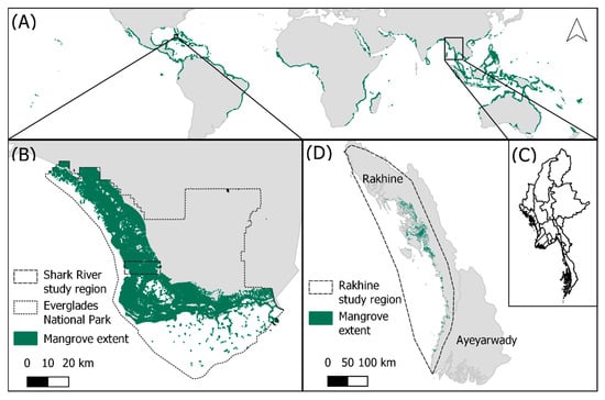
Figure 1.
(A) Global mangrove extent from the Global Mangrove Watch 2016 dataset. (B) Case study region around Shark River within the Everglades National Park in Florida. (C) The location of Rakhine and Ayeyarwady states (line-shaded) within Myanmar. (D) Case study region for Rakhine mangroves along the coast of the Rakhine state and far west coast of Ayeyarwady up to Cape Negrais.
The Rakhine mangroves ecosystem is one of four mangrove ecosystem types in Myanmar (Rakhine mangroves forest on mud) [39]. The ecosystem consists of at least 28 mangrove species, including the critically endangered Bruguiera hainseii and Sonneratia griffithii [40], and occurs across four geomorphic settings [41]. In Rakhine, anthropogenic activities including the construction of artificial sea walls, tree harvesting, and conversion to rice paddies, aquaculture, and oil palm plantations lead to extensive degradation of mangroves. These activities disrupt the natural exchange of ocean and freshwater by interrupting natural tidal, sedimentation, and salinity regimes (Figure 2) [42,43]. The region is also affected by periodic storms, although their contribution to mangrove degradation is considered low [44]. Owing to ongoing movement restrictions, in-situ data and published studies are scarce for this region, but degradation caused by these activities is clearly observable with high resolution satellite imagery (Figure 3). We modelled the extent of degradation in Rakhine using satellite imagery collected in 2017.
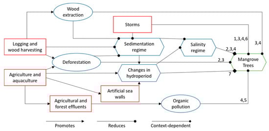
Figure 2.
Simplified conceptual model of the threats and the ecological processes relevant to mapping mangrove degradation in our analysis. Red boxes indicate threats, blue ovals represent the abiotic processes, blue hexagons represent the abiotic environment, and the green hexagon represents the biotic components of the mangrove ecosystem. Pointed arrowheads indicate positive effects, rounded arrowheads indicate negative effects, and diamond arrowheads indicate context-dependent effects. Numbers show potential satellite-derived variables to be used to detect specific ecological links contributing to mangrove degradation from Table 1. A more complete model is presented in Figure S1.
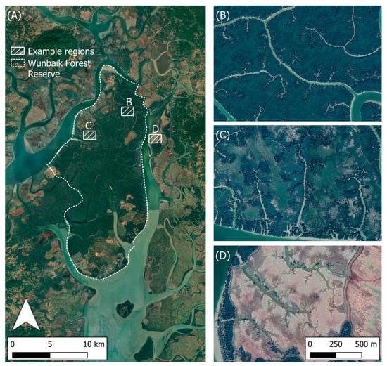
Figure 3.
Examples of mangrove ecosystem degradation in Rakhine, Myanmar. (A) High resolution imagery from Google Earth (2018) of mangroves in the region around the Wunbaik Forest Reserve, Rakhine. Zoomed in images represent examples for (B) intact, (C) degraded, and (D) collapsed classes. Image data provided by Landsat/Copernicus, CNES/Airbus, Google, and Maxar Technologies.
Our second study region is a small area of intensively-studied lagoonal mangroves along Shark River, Everglades National Park, Florida, USA (Figure 1) [41]. This ecosystem is dominated by only three mangrove species: Avicennia germinans, Laguncularia racemosa, and Rhizophora mangle. All three species occur near the mouth of Shark River, while the mangroves become progressively smaller and shorter upstream, with an increasing dominance of R. mangle, along with increasing presence of mangrove-associate Conocarpus erectus inland [45]. This ecosystem is considered relatively unaffected by direct anthropogenic impacts, but periodic disturbance by severe storms leads to extensive loss of foliage and structural damage [46,47]. We modelled the extent of degradation before (June 2016–May 2017) and after (November 2017–October 2018) a tropical cyclone (Hurricane Irma), which caused severe short-term degradation to the ecosystem [48,49].
2.2. Conceptual Model
Using information from published literature, we developed a conceptual model of mangrove ecosystems that assists in the identification of key pathways to mangrove degradation (Figure S1). In our analysis, we focused on degradation of mangrove vegetation due to its relative ease to be detected using satellites, though other aspects of the ecosystem may also represent mangrove degradation [36]. We used the conceptual model to identify satellite-derived variables and their ecological link to mangrove degradation (Table 1), helping us choose appropriate variables that are likely to change as a result of mangrove degradation. A simplified version of the conceptual model, focusing on the earth observation data available and the degradation drivers relevant to our case study regions, is presented here (Figure 2).

Table 1.
Satellite-derived variables and their ecological link to mangrove degradation. Variables were identified with a conceptual model of mangrove ecosystems (Figure 2).
2.3. Training Data
Our model sought to predict the spatial distribution of degraded mangroves, formulated as discrete classes representing ordinal states of mangrove condition. We developed a training set to reflect these states, consisting of confirmed occurrences of the three target map classes:
- intact, representing mangrove pixels with closed canopies and no visible indication of departure from natural variability at the interannual level (maintained at more than 5 years (Figure 3B);
- degraded, representing mangrove pixels with visible degradation (departure from natural variability) but with mangrove trees still present (Figure 3C);
- collapsed, representing pixels mapped as mangrove in 2016 by GMW without any evidence of the mangrove tree presence at the time of analysis (Figure 3D).
Importantly, the training data created reflects overall mangrove condition and do not necessarily reflect each of the ecological links identified in Table 1. Here, we used a closed canopy as a prerequisite to be included within the intact class. We recognise that some mangrove species may have low canopy cover even when not degraded and that this is a limitation to our model. We used high resolution Google Earth imagery collected during the dry season (available for >90% of our study areas) for the analysis years for each case study to interactively identify point locations for each class. Although the high-resolution images were only available during the dry season, our training sample should not be too affected, as mangroves are unlikely to change in appearance throughout the year. For a pixel to be labelled as intact in the training set (Figure 3B), it met the following criteria:
- part of a mangrove forest patch that is at least 5 hectares (ha) in area;
- closed canopy cover with no underlying substrate observed from Google Earth imagery;
- no obvious anthropogenic structures and disturbances observed from Google Earth imagery;
- maintained the above criteria for at least 5 years.
Pixels in the training set annotated as degraded (Figure 3C) met the criteria:
- mangrove trees can be observed in Google Earth imagery (thus not collapsed);
- low canopy cover and/or isolated trees observed from Google Earth imagery, and/or;
- browning and/or tree death observable from Google Earth imagery.
Training pixels that represented the collapsed class were necessary for Rakhine mangroves, where parts of the study area were mapped as mangroves in the GMW 2016 data [38] but did not include any mangrove trees in Google Earth imagery in 2017 (Figure 3D). This could either be due to a recent collapse of the mangrove forest (e.g., land conversion) or misclassifications in the GMW dataset. Our final training set for the Rakhine mangroves degradation model comprised 130 intact, 130 degraded points, and 60 collapsed points. Independent validation data were collected at a later stage (see Section 2.6).
Owing to the Shark River case study before/after hurricane design, we used Google Earth imagery from before and after Hurricane Irma to identify intact (early 2017) and degraded pixels (early 2018). Collapsed pixels were not necessary for this region, and our final training set here comprised 50 intact and 50 degraded points. Independent validation data were collected at a later stage (see Section 2.6).
2.4. Covariate Selection and Processing
We developed our covariate set using the conceptual model. We considered various satellites to use as data sources (Table 1), but the two main criteria were adequate spatial resolution and adequate temporal coverage. OCO-2 (Orbiting Carbon Observatory 2) and TOPEX/Poseidon had spatial resolutions that were too coarse, while GEDI (Global Ecosystem Dynamics Investigation), ECOSTRESS, and SRTM (Shuttle Radar Topography Mission) did not have data for our study period. This left Landsat, Sentinel-2, and ALOS-2 PALSAR-2 (Advanced Land Observing Satellite 2 Phased Array type L-band Synthetic Aperture Radar 2) for us to consider. Ultimately, we decided on using Landsat and ALOS-2 PALSAR-2. We omitted Sentinel-2 data because of its similarity with Landsat; any variables derived from it would have mirrored those from Landsat, leading to the indices being included twice. Between Landsat and Sentinel-2, we chose to use Landsat due to the availability of analysis-ready data with reliable cloud-masking data. The main advantage of using Sentinel-2 would have been the higher spatial resolution, though this would have been nullified as we used GMW data as our mangrove masks, which themselves were at 25 m resolution.
The final covariate set, totalling seven data layers, consisted of 30 m resolution layers processed from Landsat-8 (five covariate layers) and ALOS-2 PALSAR 2 (yearly mosaic; two covariate layers resampled to 30 m). Landsat-8 was used to create NDVI (Equation (1)), Normalised Difference Moisture Index (NDMI; Equation (2)), and Normalised Difference Water Index (NDWI; Equation (3)) layers. We chose to use derived spectral indices, as we can readily present the proposed mechanisms for each covariate using information from the literature (Table 2). For example, we expected intact mangroves to have higher NDVI and NDMI and a lower NDWI than degraded mangroves (Table 2) [50,51]. Despite mangroves being highly dynamic systems, we also expected degraded mangroves to be less temporally stable, as vegetation structure and sediment stability in degraded areas may exhibit greater temporal variability, resulting in higher standard deviation in NDVI and NDMI (Table 2) [52]. Lastly, there is evidence that L-band Synthetic Aperture Radar (SAR; available from ALOS-2 PALSAR-2) is highly correlated with mangrove biomass, where, with certain limitations, decreased backscatter values correlate to decreased biomass (Table 2) [53].
Table 2.
Satellite-derived covariates used to model mangrove degradation. The table suggests the expected mechanism for detecting mangrove degradation.
To aggregate the annual Landsat-8 data into single layers for each variable [23], we first masked clouds using the CFMask band [55], computed the three indices, and then calculated pixel-specific means (for all three indices) and standard deviations (for NDVI and NDMI only) over a one year period. ALOS-2 PALSAR-2 data were processed to yearly mosaics for both horizontal emitted, horizontal received (HH) and horizontal emitted, vertical received (HV) polarisations, and a refined Lee filter was applied to both layers [56,57]. By using annual summaries and mosaics, we minimised any sub-annual variations, such as phenology or tidal effects which may bias our classifications. All data processing was conducted in Google Earth Engine [58]. ALOS-2 PALSAR-2 data were not available on Google Earth Engine for Shark River at the time of analysis and were therefore not included in the model.
2.5. Classification Models
Due to their ease of implementation, proven ability to classify mangrove forests [35,59], and ability to capture non-linear relationships, we developed random forest classification models, one of the most commonly used algorithms provided by Google Earth Engine for classification tasks [60], to map mangrove degradation for our two case study ecosystems [61].
As a result of the ordinal nature of our three output classes and the inability of random forest models to account for ordering information [62], we formulated a two-step process for Rakhine mangroves. A random forest model was first trained to classify all pixels as intact or not intact using training data from the intact class and a merged “not-intact” class comprising both degraded and collapsed training points. We then trained a second random forest model classifying all pixels as collapsed or not using the collapsed training samples and the remaining points merged into a “not-collapsed” class. Splitting the classification models in this manner further allowed us to investigate potential differences in the variables that may be important to differentiate between intact, degraded, and collapsed mangroves. Both random forest models in Rakhine included all seven covariates layers. We selected fifty trees (ntree = 50), and mtry was set to the default value (square root of the number of variables) for both models. Landsat covariate layers were calculated from all non-cloud obstructed pixels (based on CFMask [55]) from 2017 and the filtered 2017 ALOS-2 PALSAR-2 annual mosaics and used as the covariate layers [57].
The resulting maps from these two models were combined into a single output using the rules: (i) pixels classified as intact in the first model and not collapsed in the second model were assigned a final class of intact; (ii) pixels classified as not intact and collapsed were assigned a final class of collapsed; and (iii) all remaining pixels were assigned a final class of degraded.
A single two-class random forest classifier was used to map intact and degraded pixels across the Shark River study site (as there was no need for a collapsed class in this region), producing “pre-disturbance” and “post-disturbance” maps of mangrove degradation. This random forest model included five covariate layers, as ALOS-2 PALSAR-2 data were not available on Google Earth Engine for the post-disturbance period at the time of analysis. We selected fifty trees (ntree = 50), and mtry was set to the default value (square root of the number of variables). The annual metrics before the hurricane were calculated from all non-cloud obstructed pixels (based on CFMask [55]) between 1 June 2016 and 31 May 2017, while the annual metrics after the hurricane were calculated from all non-cloud obstructed pixels between 1 November 2017 and 31 October 2018.
We also investigated the relative importance (Gini importance) of the variables that were included in each model to highlight the variables important to the classification models and whether the same variables were important for the different models [63].
2.6. Area Estimation and Accuracy Assessment
We assessed the accuracy of our model using error matrices and following best practicing procedures, ensuring the accuracy estimates were non-biased [64]. We developed an independent validation set using stratified random sampling with equal allocation for each study region (Rakhine mangroves: n = 2,700; Florida: n = 600). For Rakhine mangroves, four independent assessors (authors CKFL, CD, TAW, NJM) assigned the testing points to a class following the criteria described in Section 2.4. From the 2700 points sampled in Rakhine, 300 points were given to all four assessors to estimate agreement between assessors using Fleiss’ Kappa (not to be confused with the Kappa coefficient sometimes used to assess classification accuracy) [65,66]. The remaining 2400 were split into four equal sets, and each assessor was given a different set to validate. The 600 points sampled from Shark River were assessed by a single assessor (CKFL). The error matrices were also used to calculate the area and the confidence intervals of each class using an unbiased estimator [64].
3. Results
3.1. Degradation Distribution, Area Estimation, and Accuracy Assessment of Rakhine Mangroves
Our model suggested that 48.4% (standard error (SE) 0.8) (732km2 (SE 12)) of Rakhine mangroves were intact, 39.5% (SE 0.9) (597km2 (SE 13)) were degraded, and 12.0% (SE 0.5) (182km2 (SE 8)) collapsed. The model indicated that degradation was widespread across the entire case study region (Figure 4). The northern districts had a relatively higher proportion of degraded mangroves, with the districts of Maungtaw and Sittwe recording more than half of their mangrove’s distribution as degraded (Table 3). The southern districts of Thandwe and Bassein had the lowest percentage of degraded mangroves, though more than a quarter of the districts’ mangroves were still mapped as degraded.
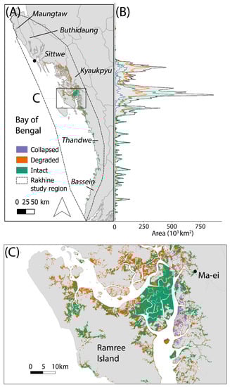
Figure 4.
(A) Mapped mangrove degradation for the Rakhine case study region. Italics denote name of districts. Dot denotes the location of Sittwe, Rakhine’s state capital. (B) Estimated area of each mapped class and total mangrove area as mapped by Global Mangrove Watch against latitude. (C) Mangrove degradation for the region surrounding the Wunbaik Forest Reserve. All maps use UTM46 at 30 m resolution.
Table 3.
Percentage of mangroves mapped as degraded per district sorted by latitude and the percentage of mangroves within each district relative to the entire Rakhine mangroves case study region.
Additionally, mangroves in Wunbaik Forest Reserve (within Kyaunkypyu district) accounted for 9.8% of the total extent of Rakhine mangroves, and despite its protected status, 25.3% of the mangroves within the forest reserve was mapped as degraded. Extensive mangrove degradation was also identified in areas surrounding the forest reserve (Table 3; Figure 4C).
Agreement between the four independent accuracy assessment analysts returned an overall Fleiss’ Kappa of 0.69 (p < 0.05; Table 4). The Kappa values were significant for all classes, though agreement was highest for collapsed (Kappa = 0.884) and lowest for degraded (Kappa = 0.559).
Table 4.
Results for Fleiss’ Kappa for four assessors for each class.
The accuracy assessment suggested that the model under-represented both intact (−4.9%) and collapsed classes (−2.0%), while the degraded class was over-represented (7.0%) (Table 5). The User’s and Producer’s accuracies for the degraded class in Rakhine were 69.3% and 81.5%, respectively and the overall model accuracy for the Rakhine was 77.6%.
Table 5.
Error matrix of the Rakhine mangroves degradation model. Cell entries represent percent of total area. Map categories are in rows while the reference categories are in columns.
For the collapse-not-collapsed model, NDMI standard deviation was the most important variable, while the HH band and the NDWI mean were the least important variables (Table 6). The intact-not-intact model had more balanced relative importance across all variables, with NDMI mean having the highest importance (Table 7). Interestingly, the standard deviation measures appear to have been more important when differentiating between whether mangroves were collapsed or not, while the mean measures were more important when differentiating between intact and not intact mangroves.
Table 6.
Relative importance of the variables for the model classifying collapsed and not-collapsed pixels for Rakhine mangroves.
Table 7.
Relative importance of the variables for the model classifying intact and not-intact pixels for Rakhine mangroves.
3.2. Degradation Distribution, Area Estimation, and Accuracy Assessment of Shark River Mangroves
Our model suggested that, before Hurricane Irma, most of the Shark River study region consisted of intact mangroves, with only 5.1% (SE 1.9) of the region classified as degraded. However, after Hurricane Irma, the percentage of mangrove area identified as degraded increased to 97.4% (SE 2.5).
Degradation after the storm was more prevalent closer to the open ocean on the south-western side of the study region, along with the shorter mangroves in the north-eastern side which were classified as degraded in both time periods. Only the central region of the study area had some remaining patches of intact mangroves after the storm (Figure 5).
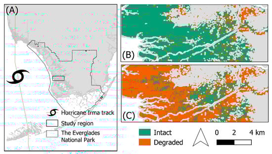
Figure 5.
Mapped mangrove degradation for the Shark River case-study region. (A) Location of Shark River study region within the Everglades National Park, showing Hurricane Irma’s track (B) Results of the degradation model for pre-Hurricane Irma (2016–2017) and (C) Post-Hurricane Irma (2017–2018).
The User’s and Producer’s accuracies for the degraded class in Shark River were 73.9% and 86.7%, respectively, and the model had an overall accuracy of 79.1% (Table 8). The accuracy assessment indicated that the model under-represented the intact mangrove 5. class and over-represented the degraded mangrove class by 8.2%. For this model, NDVI mean and NDMI mean had the highest relative importance, while NDVI standard deviation did not contribute to the model at all (Table 9). As the Shark River classification did not include a collapsed class, the model here was similar to the intact-not-intact model for Rakhine. These two models had similar relative variable importances, with the mean measures having much higher importance than the standard deviation measures.
Table 8.
Error matrix of Shark River mangrove degradation model. Cell entries represent percent of area. Map categories are in rows while the reference categories are in columns.
Table 9.
Relative importance of the variables for the model classifying intact and not-intact pixels for Shark River mangroves.
4. Discussion
Despite the need for consistently quantified measures of ecosystem degradation [2,67], few methods exist that estimate the distribution of degradation at the ecosystem-scale without resource-intensive field data. We present a method that enables large scale assessments of ecosystem condition using freely available satellite data linked to a defined ecosystem conceptual, developing different classification models suitable for our two case study regions. We found that more than half of the mangroves in our Rakhine study area were identified as degraded or collapsed, while a single intense storm caused extensive mangrove degradation along Shark River. Our study highlights the feasibility of moving beyond area-based (i.e., ecosystem cover only) goals for conservation, which can greatly underestimate negative impacts of ecosystem change on biodiversity and dependent ecosystem services [68] by quantifying the various states of mangrove degradation.
The two case studies used the same conceptual model to build two different classification models, with slight differences in the data included. Due to this, the mapped degraded classes in our two case studies may not be directly quantitatively comparable but follow the same conceptual definition and thus can both be used to investigate extent of mangrove degradation. Our models were both able to detect mangrove degradation in both study regions despite the different classification models and drivers of degradation. We found that the highest incidence of degradation in Rakhine mangroves were in the north of the study region, suggesting more extensive urban development in this region near to the state capital of Sittwe is leading to more extensive mangrove degradation. This result highlights the continued negative impact of anthropogenic activities on the mangroves in the region, including physical damage to the forests via wood harvesting and changes to water flows caused by the construction of dykes and seawalls, which are the initial stages in developing aquaculture [44]. This degradation combined with the continued mangrove loss detected in the region [43] reveals that Rakhine’s mangrove forests are likely to continue to be degraded if no supplementary conservation actions are implemented.
In Shark River, our model identified the widespread impacts of a single intense storm event, which caused widespread defoliation and mortality. Before the storm, we assumed that all mangroves within a single case study region had the same classification criteria; however, our model suggested that 5.1% of the study region was already degraded. Mangroves mapped as degraded were found further inland on the north-eastern side of the study region, where mangroves are dominated by the stunted R. mangle, mixed with herbaceous vegetation (Figure 5), and are consistently shorter than other mangroves in the study region due to being chronically stressed due to limited water or nutrient availability [69]. Hurricane Irma in 2017 led to an additional 92.3% of the region’s mangroves becoming degraded, with degradation more extensive near the coastline as the storm winds caused more damage to the taller mangroves [49]. The degradation observed here may particularly be a cause for concern if storms increase in frequency or intensity under climate change, particularly in regions with prolonged recovery rates [49,70].
In our classification models, we included annual summaries of various Landsat-derived indices along with ALOS-2 PALSAR-2 annual mosaic for Rakhine. The results showed that different variables were important in differentiating between intact and not-intact mangroves and collapsed and not-collapsed mangroves (Table 6, Table 7 and Table 9). The importance of the mean measures for differentiating between intact and not intact mangroves suggest that the actual value of the indices is more important for intact mangroves, which likely have much higher NDVI and NDMI values. On the other hand, the stability of the values is more important when differentiating between whether mangroves have collapsed or not. The ALOS-2 PALSAR-2 data were also important in the intact-not-intact model, suggesting that it could have been a useful source of information for the Shark River analysis.
By using a conceptual model to select ecological-meaningful variables for our classification models, we can much more easily interpret the results of the variable importances from the models and can directly use them to investigate whether the model behaviour matches the mechanisms proposed to affect mangrove degradation (Table 2). Moreover, building a conceptual model prior to classification highlighted the data required to map mangrove degradation and thus any data gaps and limitations when no suitable data were available as input into the classification models. In the case studies here, no suitable data to represent evaporative stress were included in our classification models despite their potential importance in detecting mangrove degradation (Table 1) [46].
Despite providing ecologically meaningful inferences from the developed conceptual mangrove ecosystem model and high quantitative model accuracies here, our present approach has scope for further development. The data we used as explanatory variables in our models were snapshots and did not take long-term (>one year) temporal trends into account. As a result, potential ecosystem recovery was not assessed for either case study. As such, our results here did not capture mangrove recovery in Shark River [49]. Similarly, our results for the Rakhine mangroves did not explicitly show a lack of recovery from the anthropogenic threats. To produce results that track ecosystem degradation over longer time periods, the models trained here can be applied to data collected by the same satellite sensors at regular time intervals. Results produced in this manner allow us to capture changes in mapped degradation, revealing potential recovery or continued degradation through time. Using time-series maps produced this way can also help us differentiate between mangroves that originally had close canopies and became degraded and mangroves that naturally have open canopies.
Our models had accuracies of 77% and 79% and overestimated the extent of mangrove degradation for both regions (Table 3). Inaccuracies were primarily due to the relatively coarse spatial resolution of the underlying data, which is several times larger than a single tree canopy. In cases where there were multiple land cover types within a single pixel, such as mangroves along water courses (water and mangrove in a single pixel), or when there were two or more degradation classes within a single pixel (for example, the border between a degraded and intact mangroves), the model tended to classify these pixels as degraded. Additional commission errors in the degraded class appeared to be due to pixels that were initially misclassified in the GMW base map (e.g., other forest types, greenery in villages). Our models assumed that all input pixels were mangrove pixels, meaning these pixels misclassified by GMW did not fit into any of the criteria listed in Section 2.3. These pixels were labelled as collapsed by assessors, though it was unlikely for the models to be able to effectively classify them, as they were not developed to classify non-mangrove land cover types. Additionally, the high-resolution Google Earth imagery used for training and validation were only available during the dry season, but the data used as covariates in our classification models were summarized over the entire year after cloud masking. This could potentially bias our results, though it is unlikely mangroves will appear substantially different throughout the year in high-resolution imagery. Despite these misclassifications, we believe overestimating degradation is preferable to the alternative, as it provides more conservative estimates following a precautionary approach.
Given the above sources of classification error, future development of the models can improve the accuracy in several ways. Firstly, we can integrate an additional step by explicitly modelling other land cover classes that help reduce uncertainties in the underlying mangrove cover datasets. Secondly, data with finer spatial resolution, ideally those finer than a single tree canopy, will help us and understand and minimise errors due to mixed pixels, though this can lead to additional sources of errors from shadows and noise. Thirdly, producing annual maps of mangrove degradation using the same models can allow us to compare extent of degradation through time, providing information of potential mangrove degradation and recovery. Lastly, modelling a continuous class of degradation (e.g., from low to high levels), as opposed to simply classifying degradation into a single class, will allow us to capture the severity of degradation as a continuous response variable. This will likely require extensive field data collected explicitly quantifying the (relative) severity of degradation as the objective. Examples will be data that capture ecosystem composition, such as plant surveys specifying species richness, ecosystem structure, such as canopy cover measurements using a Cajanus tube [71], and ecosystem function, such as estimating plot level net primary productivity. Additionally, field data can also be incorporated as explanatory variables, providing additional information that captures the specific components highlighted by the conceptual model. For example, data for soil salinity within mangrove forests at various stages of degradation can be used to provide information about the salinity regime to the models, while tide gauges can provide precise information on the hydroperiod of the study site. Not only will these data increase the accuracy of the models, spatially explicit maps of ecosystem degradation severity will also provide additional information that the classification approach used here cannot provide.
5. Conclusions
The world’s ecosystems continue to be threatened as the human population and activity rises [2,72]. In this study, we provided a method of developing quantitative classification models that are ecologically relevant to map mangrove ecosystem degradation using freely available satellite data. Our model, which quantifies the distribution of observed mangrove forest degradation, can be adapted to assess and map conditions for a range of ecosystem types globally. Such an approach promotes a robust, transparent, and repeatable process for assessing the status of ecosystems and to move beyond area-based ecosystem assessments. The findings here and the results produced using this method would support efforts to conduct ecosystem risk assessments, such as the International Union for Conservation of Nature (IUCN) Red List of Ecosystems [2] and global biodiversity targets such as the post-2020 Global Biodiversity Framework [6] and the UN Sustainable Development Goals [7]. Additionally, the System of Environmental Economic Accounting measures ecosystem condition and capacity to provide ecosystem services [8], and the United Nations Reduced Emissions from Deforestation and Degradation (REDD+) program focuses on forests’ capacity for carbon storage [73], all of which should be informed by maps of ecosystem degradation, providing critical nuances that are lost if only ecosystem extent change is considered.
Supplementary Materials
The following are available online at https://www.mdpi.com/article/10.3390/rs13112047/s1, Figure S1: Detailed mangrove conceptual model highlighting threats and processes affecting mangrove degradation. Red boxes indicate threats, blue ovals represent the abiotic processes, blue hexagons represent the abiotic environment, and green hexagons represent the biotic components of the mangrove ecosystem. Pointed arrowheads indicate positive effects, rounded arrowheads indicate negative effects, and diamond arrowheads indicate context-dependent effects.
Author Contributions
Conceptualization, C.K.F.L., C.D., E.N., T.E.F., D.L., N.T., T.A.W. and N.J.M.; methodology, C.K.F.L., C.D., T.E.F., D.L., N.T., T.A.W. and N.J.M.; validation, C.K.F.L., C.D., T.A.W. and N.J.M.; formal analysis, C.K.F.L., N.J.M.; writing—original draft preparation, C.K.F.L., C.D., E.N. and N.J.M.; writing—review and editing, C.K.F.L., C.D., E.N., T.E.F., D.L., N.T., T.A.W. and N.J.M.; All authors have read and agreed to the published version of the manuscript.
Funding
C.K.F.L. was funded by the Australian Government Research Training Program Scholarship. N.J.M. was supported by an Australian Research Council Discovery Early Career Research Award DE190100101. E.N. was supported by Veski and the Office of the Chief scientist of Victoria (IWF01). N.J.M. and E.N. were supported by the Australian Research Council (FT190100234 to E.N.; LP170101143 to E.N., N.J.M.). C.D. was supported by the AXA Research Fund. T.E.F, N.T., and D.L. were funded by the NASA Carbon Monitoring System Program Project “Estimating Total Ecosystem Carbon in Blue Carbon and Tropical Peatland Ecosystems” (16-CMS16-0073).
Data Availability Statement
A repository containing a Google Earth Engine script demonstrating the training of the random forest classification models used in this study is available under these links: https://code.earthengine.google.com/66d871bd8d597c5334e983dd6c14688f (accessed on 19 May 2021) (Rakhine). https://code.earthengine.google.com/3b8306b7faa62d03df56dcb623d36e4b (accessed on 19 May 2021) (Shark River) and https://github.com/calvinkflee/mangrove_degradation (accessed on 19 May 2021). The degradation maps for Rakhine mangroves, pre- and post-Irma Shark River mangroves degradation are available here: 10.6084/m9.figshare.13071812.
Acknowledgments
Landsat data were provided by U.S. Geological Survey. ALOS-2 PALSAR-2 data were provided by Japan Aerospace Exploration Agency.
Conflicts of Interest
The authors declare no conflict of interest.
References
- Millennium Ecosystem Assessment. Ecosystem and Human Well-Being; Island Press: Washington, DC, USA, 2005. [Google Scholar]
- Keith, D.A.; Rodríguez, J.P.; Rodríguez-Clark, K.M.; Nicholson, E.; Aapala, K.; Alonso, A.; Asmussen, M.; Bachman, S.; Basset, A.; Barrow, E.G.; et al. Scientific Foundations for an IUCN Red List of Ecosystems. PLoS ONE 2013, 8, e62111. [Google Scholar] [CrossRef] [PubMed]
- Mace, G.M.; Norris, K.; Fitter, A.H. Biodiversity and Ecosystem Services: A Multilayered Relationship. Trends Ecol. Evol. 2012, 27, 19–26. [Google Scholar] [CrossRef]
- Cardinale, B.J.; Duffy, J.E.; Gonzalez, A.; Hooper, D.U.; Perrings, C.; Venail, P.; Narwani, A.; Mace, G.M.; Tilman, D.; Wardle, D.A.; et al. Biodiversity Loss and Its Impact on Humanity. Nature 2012, 486, 59–67. [Google Scholar] [CrossRef] [PubMed]
- Costanza, R.; de Groot, R.; Sutton, P.; van der Ploeg, S.; Anderson, S.J.; Kubiszewski, I.; Farber, S.; Turner, R.K. Changes in the Global Value of Ecosystem Services. Glob. Environ. Chang. 2014, 26, 152–158. [Google Scholar] [CrossRef]
- CBD. Observations on Potential Elements for the Post-2020 Global Biodiversity Framework. In Proceedings of the Convention on Biological Diversity, Twenty-Third Meeting, Montreal, QC, Canada, 25–29 November 2019. [Google Scholar]
- UN High Commissioner for Refugees (UNHCR). The Sustainable Development Goals and Addressing Statelessness, March 2017. Available online: https://www.refworld.org/docid/58b6e3364.html (accessed on 23 May 2020).
- UN. System of Environmental-Economic Accounting 2012: Experimental Ecosystem Accounting; United Nations: New York, NY, USA, 2014. [Google Scholar]
- Sutton, P.C.; Anderson, S.J.; Costanza, R.; Kubiszewski, I. The Ecological Economics of Land Degradation: Impacts on Ecosystem Service Values. Ecol. Econ. 2016, 129, 182–192. [Google Scholar] [CrossRef]
- Grantham, H.S.; Duncan, A.; Evans, T.D.; Jones, K.; Beyer, H.; Schuster, R.; Walston, J.; Ray, J.; Robinson, J.; Callow, M.; et al. Modification of Forests by People Means Only 40% of Remaining Forests Have High Ecosystem Integrity. bioRxiv 2020. Available online: https://www.biorxiv.org/content/10.1101/2020.03.05.978858v4 (accessed on 6 October 2020). [CrossRef]
- Tulloch, V.J.D.; Tulloch, A.I.T.; Visconti, P.; Halpern, B.S.; Watson, J.E.M.; Evans, M.C.; Auerbach, N.A.; Barnes, M.; Beger, M.; Chadès, I.; et al. Why Do We Map Threats? Linking Threat Mapping with Actions to Make Better Conservation Decisions. Front. Ecol. Environ. 2015, 13, 91–99. [Google Scholar] [CrossRef]
- Ward, R.D.; Friess, D.A.; Day, R.H.; MacKenzie, R.A. Impacts of Climate Change on Mangrove Ecosystems: A Region by Region Overview. Ecosyst. Health Sustain. 2016, 2. [Google Scholar] [CrossRef]
- Duncan, C.; Owen, H.J.F.; Thompson, J.R.; Koldewey, H.J.; Primavera, J.H.; Pettorelli, N. Satellite Remote Sensing to Monitor Mangrove Forest Resilience and Resistance to Sea Level Rise. Methods Ecol. Evol. 2018, 9, 1837–1852. [Google Scholar] [CrossRef]
- Hooper, D.U.; Adair, E.C.; Cardinale, B.J.; Byrnes, J.E.K.; Hungate, B.A.; Matulich, K.L.; Gonzalez, A.; Duffy, J.E.; Gamfeldt, L.; O’Connor, M.I. A Global Synthesis Reveals Biodiversity Loss as a Major Driver of Ecosystem Change. Nature 2012, 486, 105–108. [Google Scholar] [CrossRef]
- Reygadas, Y.; Jensen, J.L.R.; Moisen, G.G. Forest Degradation Assessment Based on Trend Analysis of MODIS-Leaf Area Index: A Case Study in Mexico. Remote Sens. 2019, 11, 2503. [Google Scholar] [CrossRef]
- Bai, Z.G.; Dent, D.L.; Olsson, L.; Schaepman, M.E. Proxy Global Assessment of Land Degradation. Soil Use Manag. 2008, 24, 223–234. [Google Scholar] [CrossRef]
- Noss, R.F. Indicators for Monitoring Biodiversity: A Hierarchical Approach. Conserv. Biol. 1990, 4, 355–364. [Google Scholar] [CrossRef]
- FAO. Global Forest Resources Assessment 2020; FAO: Rome, Italy, 2020; ISBN 978-925-132-974-0. [Google Scholar]
- Potapov, P.; Yaroshenko, A.; Turubanova, S.; Dubinin, M.; Laestadius, L.; Thies, C.; Aksenov, D.; Egorov, A.; Yesipova, Y.; Glushkov, I.; et al. Mapping the World’s Intact Forest Landscapes by Remote Sensing. Ecol. Soc. 2008, 13. [Google Scholar] [CrossRef]
- Jakobsson, S.; Töpper, J.P.; Evju, M.; Framstad, E.; Lyngstad, A.; Pedersen, B.; Sickel, H.; Sverdrup-Thygeson, A.; Vandvik, V.; Velle, L.G.; et al. Setting Reference Levels and Limits for Good Ecological Condition in Terrestrial Ecosystems—Insights from a Case Study Based on the IBECA Approach. Ecol. Indic. 2020, 116, 106492. [Google Scholar] [CrossRef]
- Murray, N.J.; Keith, D.A.; Bland, L.M.; Ferrari, R.; Lyons, M.B.; Lucas, R.; Pettorelli, N.; Nicholson, E. The Role of Satellite Remote Sensing in Structured Ecosystem Risk Assessments. Sci. Total Environ. 2018, 619, 249–257. [Google Scholar] [CrossRef]
- Taillie, P.J.; Roman-Cuesta, R.; Lagomasino, D.; Cifuentes-Jara, M.; Fatoyinbo, T.; Ott, L.E.; Poulter, B. Widespread Mangrove Damage Resulting from the 2017 Atlantic Mega Hurricane Season. Environ. Res. Lett. 2020, 15, 064010. [Google Scholar] [CrossRef]
- Potapov, P.; Tyukavina, A.; Turubanova, S.; Talero, Y.; Hernandez-Serna, A.; Hansen, M.C.; Saah, D.; Tenneson, K.; Poortinga, A.; Aekakkararungroj, A.; et al. Annual Continuous Fields of Woody Vegetation Structure in the Lower Mekong Region from 2000–2017 Landsat Time-Series. Remote Sens. Environ. 2019, 232, 111278. [Google Scholar] [CrossRef]
- Mondal, P.; McDermid, S.S.; Qadir, A. A Reporting Framework for Sustainable Development Goal 15: Multi-Scale Monitoring of Forest Degradation Using MODIS, Landsat and Sentinel Data. Remote Sens. Environ. 2020, 237, 111592. [Google Scholar] [CrossRef]
- Yuan, J.; Cohen, M.J. Remote Detection of Ecosystem Degradation in the Everglades Ridge-Slough Landscape. Remote Sens. Environ. 2020, 247, 111917. [Google Scholar] [CrossRef]
- Zhuravleva, I.; Turubanova, S.; Potapov, P.; Hansen, M.; Tyukavina, A.; Minnemeyer, S.; Laporte, N.; Goetz, S.; Verbelen, F.; Thies, C. Satellite-Based Primary Forest Degradation Assessment in the Democratic Republic of the Congo, 2000–2010. Environ. Res. Lett. 2013, 8, 024034. [Google Scholar] [CrossRef]
- Araújo, M.B.; Anderson, R.P.; Márcia Barbosa, A.; Beale, C.M.; Dormann, C.F.; Early, R.; Garcia, R.A.; Guisan, A.; Maiorano, L.; Naimi, B.; et al. Standards for Distribution Models in Biodiversity Assessments. Sci. Adv. 2019, 5, eaat4858. [Google Scholar] [CrossRef] [PubMed]
- Bland, L.B.; Keith, D.A.; Miller, R.M.; Murray, N.J.; Rodríguez, J.P. Guidelines for the Application of IUCN Red List of Ecosystems Categories and Criteria; Version 1.1; IUCN: Gland, Switzerland, 2017. [Google Scholar]
- Zador, S.G.; Gaichas, S.K.; Kasperski, S.; Ward, C.L.; Blake, R.E.; Ban, N.C.; Himes-Cornell, A.; Koehn, J.Z. Linking Ecosystem Processes to Communities of Practice through Commercially Fished Species in the Gulf of Alaska. ICES J. Mar. Sci. 2017, 74, 2024–2033. [Google Scholar] [CrossRef]
- Lee, S.Y.; Primavera, J.H.; Dahdouh-Guebas, F.; McKee, K.; Bosire, J.O.; Cannicci, S.; Diele, K.; Fromard, F.; Koedam, N.; Marchand, C.; et al. Ecological Role and Services of Tropical Mangrove Ecosystems: A Reassessment. Glob. Ecol. Biogeogr. 2014, 23, 726–743. [Google Scholar] [CrossRef]
- Richards, D.R.; Friess, D.A. Rates and Drivers of Mangrove Deforestation in Southeast Asia, 2000–2012. Proc. Natl. Acad. Sci. USA 2016, 113, 344–349. [Google Scholar] [CrossRef] [PubMed]
- Veettil, B.K.; Pereira, S.F.R.; Quang, N.X. Rapidly Diminishing Mangrove Forests in Myanmar (Burma): A Review. Hydrobiologia 2018, 822, 19–35. [Google Scholar] [CrossRef]
- Valiela, I.; Bowen, J.L.; York, J.K. Mangrove Forests: One of the World’s Threatened Major Tropical Environments. Bioscience 2001, 51, 807–815. [Google Scholar] [CrossRef]
- Hamilton, S.E.; Casey, D. Creation of a High Spatio-Temporal Resolution Global Database of Continuous Mangrove Forest Cover for the 21st Century (CGMFC-21). Glob. Ecol. Biogeogr. 2016, 25, 729–738. [Google Scholar] [CrossRef]
- Goldberg, L.; Lagomasino, D.; Thomas, N.; Fatoyinbo, T. Global Declines in Human-driven Mangrove Loss. Glob. Chang. Biol. 2020, 26, 5844–5855. [Google Scholar] [CrossRef]
- Wang, W.; Fu, H.; Lee, S.Y.; Fan, H.; Wang, M. Can Strict Protection Stop the Decline of Mangrove Ecosystems in China? From Rapid Destruction to Rampant Degradation. Forests 2020, 11, 55. [Google Scholar] [CrossRef]
- Wang, L.; Jia, M.; Yin, D.; Tian, J. A Review of Remote Sensing for Mangrove Forests: 1956–2018. Remote Sens. Environ. 2019, 231, 111223. [Google Scholar] [CrossRef]
- Bunting, P.; Rosenqvist, A.; Lucas, R.; Rebelo, L.-M.; Hilarides, L.; Thomas, N.; Hardy, A.; Itoh, T.; Shimada, M.; Finlayson, C. The Global Mangrove Watch—A New 2010 Global Baseline of Mangrove Extent. Remote Sens. 2018, 10, 1669. [Google Scholar] [CrossRef]
- Murray, N.J.; Keith, D.A.; Duncan, A.; Tizard, R.; Ferrer-Paris, J.R.; Worthington, T.A.; Armstrong, K.; Hlaing, N.; Htut, W.T.; Oo, A.H.; et al. Myanmar’s Terrestrial Ecosystems: Status, Threats and Conservation Opportunities. Biol. Conserv. 2020, 252, 108834. [Google Scholar] [CrossRef]
- Myint, W.; Stanley, D.O. The Mangrove Vegetation of Wunbaik Reserved Forest; FAO-UN: Rome, Italy, 2011. [Google Scholar]
- Worthington, T.A.; Zu Ermgassen, P.S.E.; Friess, D.A.; Krauss, K.W.; Lovelock, C.E.; Thorley, J.; Tingey, R.; Woodroffe, C.D.; Bunting, P.; Cormier, N.; et al. A Global Biophysical Typology of Mangroves and Its Relevance for Ecosystem Structure and Deforestation. Sci. Rep. 2020, 10. [Google Scholar] [CrossRef] [PubMed]
- Saw, A.A.; Kanzaki, M. Local Livelihoods and Encroachment into a Mangrove Forest Reserve: A Case Study of the Wunbaik Reserved Mangrove Forest, Myanmar. Procedia Environ. Sci. 2015, 28, 483–492. [Google Scholar] [CrossRef][Green Version]
- De Alban, J.D.T.; Jamaludin, J.; Wong de Wen, D.; Than, M.M.; Webb, E.L. Improved Estimates of Mangrove Cover and Change Reveal Catastrophic Deforestation in Myanmar. Environ. Res. Lett. 2020, 15, 034034. [Google Scholar] [CrossRef]
- Storey, D. A Socio-Economic Assessment of Mangroves Areas in North Rakhine State; REACH: Geneva, Switzerland, 2015; p. 51. [Google Scholar]
- Chen, R.; Twilley, R.R. Patterns of Mangrove Forest Structure and Soil Nutrient Dynamics along the Shark River Estuary, Florida. Estuaries 1999, 22, 955. [Google Scholar] [CrossRef]
- Lagomasino, D.; Price, R.M.; Whitman, D.; Melesse, A.; Oberbauer, S.F. Spatial and Temporal Variability in Spectral-Based Surface Energy Evapotranspiration Measured from Landsat 5TM across Two Mangrove Ecotones. Agric. For. Meteorol. 2015, 213, 304–316. [Google Scholar] [CrossRef]
- Han, X.; Feng, L.; Hu, C.; Kramer, P. Hurricane-Induced Changes in the Everglades National Park Mangrove Forest: Landsat Observations between 1985 and 2017. J. Geophys. Res. Biogeosci. 2018, 123, 3470–3488. [Google Scholar] [CrossRef]
- Zhang, C.; Durgan, S.D.; Lagomasino, D. Modeling Risk of Mangroves to Tropical Cyclones: A Case Study of Hurricane Irma. Estuar. Coast. Shelf Sci. 2019, 224, 108–116. [Google Scholar] [CrossRef]
- Lagomasino, D.; Fatoyinbo, L.; Castaneda, E.; Cook, B.; Montesano, P.; Neigh, C.; Corp, L.; Ott, L.; Chavez, S.; Morton, D. Storm Surge, Not Wind, Caused Mangrove Dieback in Southwest Florida Following Hurricane Irma. EarthArXiv 2020. Available online: https://eartharxiv.org/repository/view/159/ (accessed on 22 July 2020). [CrossRef]
- Kovacs, J.M.; Flores-Verdugo, F.; Wang, J.; Aspden, L.P. Estimating Leaf Area Index of a Degraded Mangrove Forest Using High Spatial Resolution Satellite Data. Aquat. Bot. 2004, 80, 13–22. [Google Scholar] [CrossRef]
- Lucas, R.; Van De Kerchove, R.; Otero, V.; Lagomasino, D.; Fatoyinbo, L.; Omar, H.; Satyanarayana, B.; Dahdouh-Guebas, F. Structural Characterisation of Mangrove Forests Achieved through Combining Multiple Sources of Remote Sensing Data. Remote Sens. Environ. 2020, 237, 111543. [Google Scholar] [CrossRef]
- Verbesselt, J.; Umlauf, N.; Hirota, M.; Holmgren, M.; Van Nes, E.H.; Herold, M.; Zeileis, A.; Scheffer, M. Remotely Sensed Resilience of Tropical Forests. Nat. Clim. Chang. 2016, 6, 1028–1031. [Google Scholar] [CrossRef]
- Cornforth, W.; Fatoyinbo, T.; Freemantle, T.; Pettorelli, N. Advanced Land Observing Satellite Phased Array Type L-Band SAR (ALOS PALSAR) to Inform the Conservation of Mangroves: Sundarbans as a Case Study. Remote Sens. 2013, 5, 224–237. [Google Scholar] [CrossRef]
- Kuenzer, C.; Bluemel, A.; Gebhardt, S.; Quoc, T.V.; Dech, S. Remote Sensing of Mangrove Ecosystems: A Review. Remote Sens. 2011, 3, 878–928. [Google Scholar] [CrossRef]
- Zhu, Z.; Qiu, S.; He, B.; Deng, C. Cloud and Cloud Shadow Detection for Landsat Images: The Fundamental Basis for Analyzing Landsat Time Series. In Remote Sensing Time Series Image Processing; CRC Press: Boca Raton, FL, USA, 2018; pp. 25–46. [Google Scholar]
- JAXA. Global 25 m Resolution PALSAR-2/PALSAR Mosaic and Forest/Non-Forest Map (FNF) Dataset Description 2019. Available online: https://www.eorc.jaxa.jp/ALOS/en/palsar_fnf/DatasetDescription_PALSAR2_Mosaic_FNF_revJ.pdf (accessed on 20 May 2021).
- Yommy, A.S.; Liu, R.; Wu, A.S. SAR Image Despeckling Using Refined Lee Filter. In Proceedings of the 7th International Conference on Intelligent Human-Machine Systems and Cybernetics (IHMSC), Hangzhou, China, 26–27 August 2015; Volume 2, pp. 260–265. [Google Scholar]
- Gorelick, N.; Hancher, M.; Dixon, M.; Ilyushchenko, S.; Thau, D.; Moore, R. Google Earth Engine: Planetary-Scale Geospatial Analysis for Everyone. Remote Sens. Environ. 2017, 202, 18–27. [Google Scholar] [CrossRef]
- Thomas, N.; Bunting, P.; Lucas, R.; Hardy, A.; Rosenqvist, A.; Fatoyinbo, T. Mapping Mangrove Extent and Change: A Globally Applicable Approach. Remote Sens. 2018, 10, 1466. [Google Scholar] [CrossRef]
- Tamiminia, H.; Salehi, B.; Mahdianpari, M.; Quackenbush, L.; Adeli, S.; Brisco, B. Google Earth Engine for Geo-Big Data Applications: A Meta-Analysis and Systematic Review. ISPRS J. Photogramm. Remote Sens. 2020, 164, 152–170. [Google Scholar] [CrossRef]
- Belgiu, M.; Drăguţ, L. Random Forest in Remote Sensing: A Review of Applications and Future Directions. ISPRS J. Photogramm. Remote Sens. 2016, 114, 24–31. [Google Scholar] [CrossRef]
- Janitza, S.; Tutz, G.; Boulesteix, A.-L. Random Forest for Ordinal Responses: Prediction and Variable Selection. Comput. Stat. Data Anal. 2016, 96, 57–73. [Google Scholar] [CrossRef]
- Menze, B.H.; Kelm, B.M.; Masuch, R.; Himmelreich, U.; Bachert, P.; Petrich, W.; Hamprecht, F.A. A Comparison of Random Forest and Its Gini Importance with Standard Chemometric Methods for the Feature Selection and Classification of Spectral Data. BMC Bioinform. 2009, 10, 213. [Google Scholar] [CrossRef] [PubMed]
- Olofsson, P.; Foody, G.M.; Herold, M.; Stehman, S.V.; Woodcock, C.E.; Wulder, M.A. Good Practices for Estimating Area and Assessing Accuracy of Land Change. Remote Sens. Environ. 2014, 148, 42–57. [Google Scholar] [CrossRef]
- Murray, N.J.; Phinn, S.R.; DeWitt, M.; Ferrari, R.; Johnston, R.; Lyons, M.B.; Clinton, N.; Thau, D.; Fuller, R.A. The Global Distribution and Trajectory of Tidal Flats. Nature 2019, 565, 222–225. [Google Scholar] [CrossRef] [PubMed]
- Fleiss, J.L. Measuring Nominal Scale Agreement among Many Raters. Psychol. Bull. 1971, 76, 378–382. [Google Scholar] [CrossRef]
- Ghazoul, J.; Burivalova, Z.; Garcia-Ulloa, J.; King, L.A. Conceptualizing Forest Degradation. Trends Ecol. Evol. 2015, 30, 622–632. [Google Scholar] [CrossRef] [PubMed]
- Maxwell, S.L.; Cazalis, V.; Dudley, N.; Hoffmann, M.; Rodrigues, A.S.L.; Stolton, S.; Visconti, P.; Woodley, S.; Kingston, N.; Lewis, E.; et al. Area-Based Conservation in the Twenty-First Century. Nature 2020, 586, 217–227. [Google Scholar] [CrossRef]
- Lugo, A.E. Mangrove Ecosystems: Successional or Steady State? Biotropica 1980, 12, 65. [Google Scholar] [CrossRef]
- IPCC. Climate Change 2014: Impacts, Adaptation, and Vulnerability. Part A: Global and Sectoral Aspects; Contribution of Working Group II to the Fifth Assessment Report of the Intergovernmental Panel on Climate Change; Field, C.B., Barros, V.R., Dokken, D.J., Mach, K.J., Mastrandrea, M.D., Bilir, T.E., Chatterjee, M., Ebi, K.L., Estrada, Y.O., Genova, R.C., et al., Eds.; Cambridge University Press: Cambridge, UK; New York, NY, USA, 2014. [Google Scholar]
- Korhonen, L.; Korhonen, K.T.; Rautiainen, M.; Stenberg, P. Estimation of Forest Canopy Cover: A Comparison of Field Measurement Techniques. Silva Fenn. 2006, 40, 577–588. [Google Scholar] [CrossRef]
- Butchart, S.H.M.; Walpole, M.; Collen, B.; van Strien, A.; Scharlemann, J.P.W.; Almond, R.E.A.; Baillie, J.E.M.; Bomhard, B.; Brown, C.; Bruno, J.; et al. Global Biodiversity: Indicators of Recent Declines. Science 2010, 328, 1164–1168. [Google Scholar] [CrossRef]
- UNFCCC. Key Decisions Relevant for Reducing Emissions from Deforestation and Forest Degradation in Developing Countries (REDD+); United Nations Framework Convention on Climate Change Secretariat: Bonn, Germany, 2016. [Google Scholar]


Publisher’s Note: MDPI stays neutral with regard to jurisdictional claims in published maps and institutional affiliations. |
© 2021 by the authors. Licensee MDPI, Basel, Switzerland. This article is an open access article distributed under the terms and conditions of the Creative Commons Attribution (CC BY) license (https://creativecommons.org/licenses/by/4.0/).