
Partition of Marine Environment Dynamics According to Remote Sensing Reflectance and Relations of Dynamics to Physical Factors


Abstract
:1. Introduction
2. Material
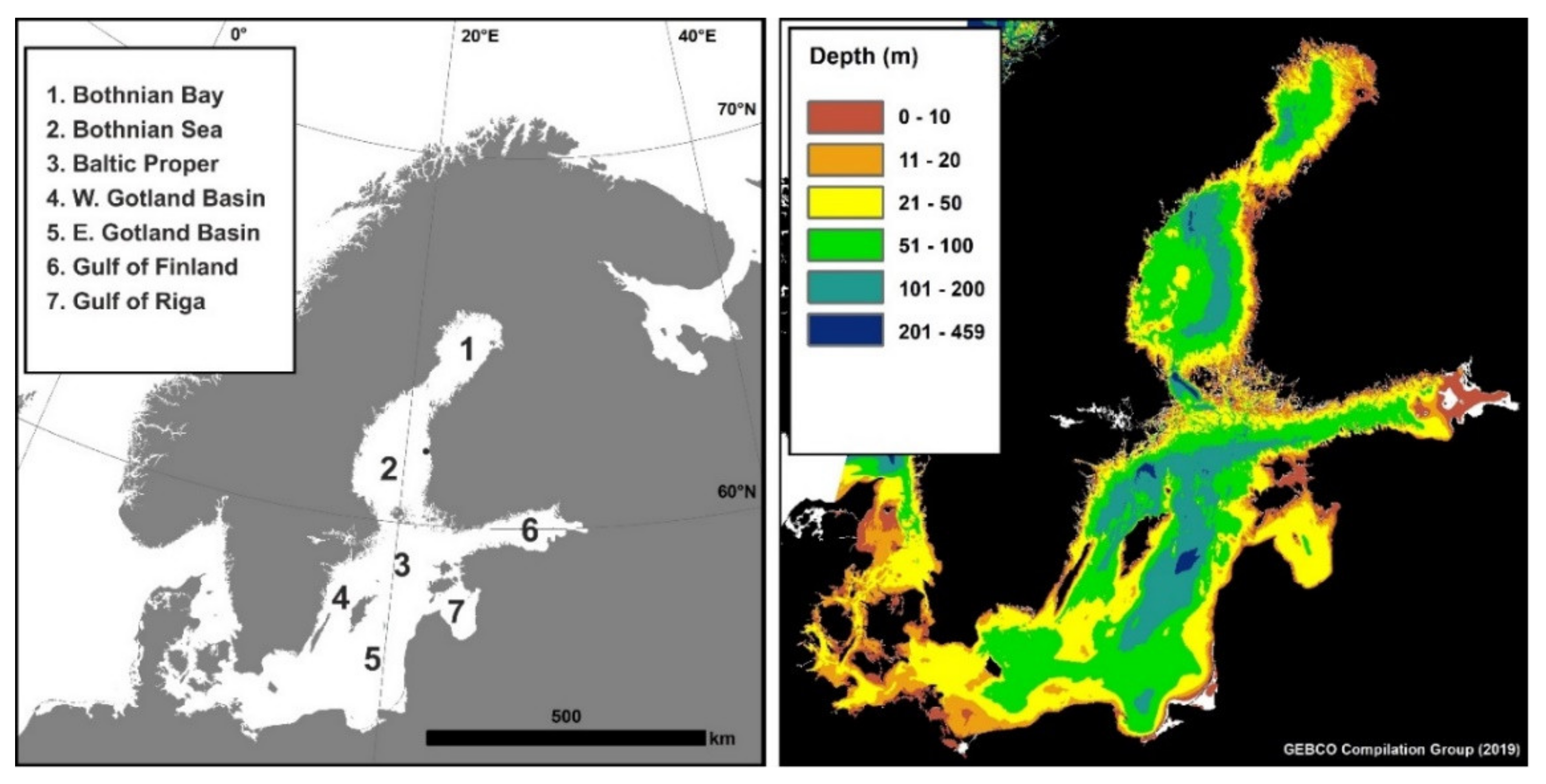
2.1. Study Area
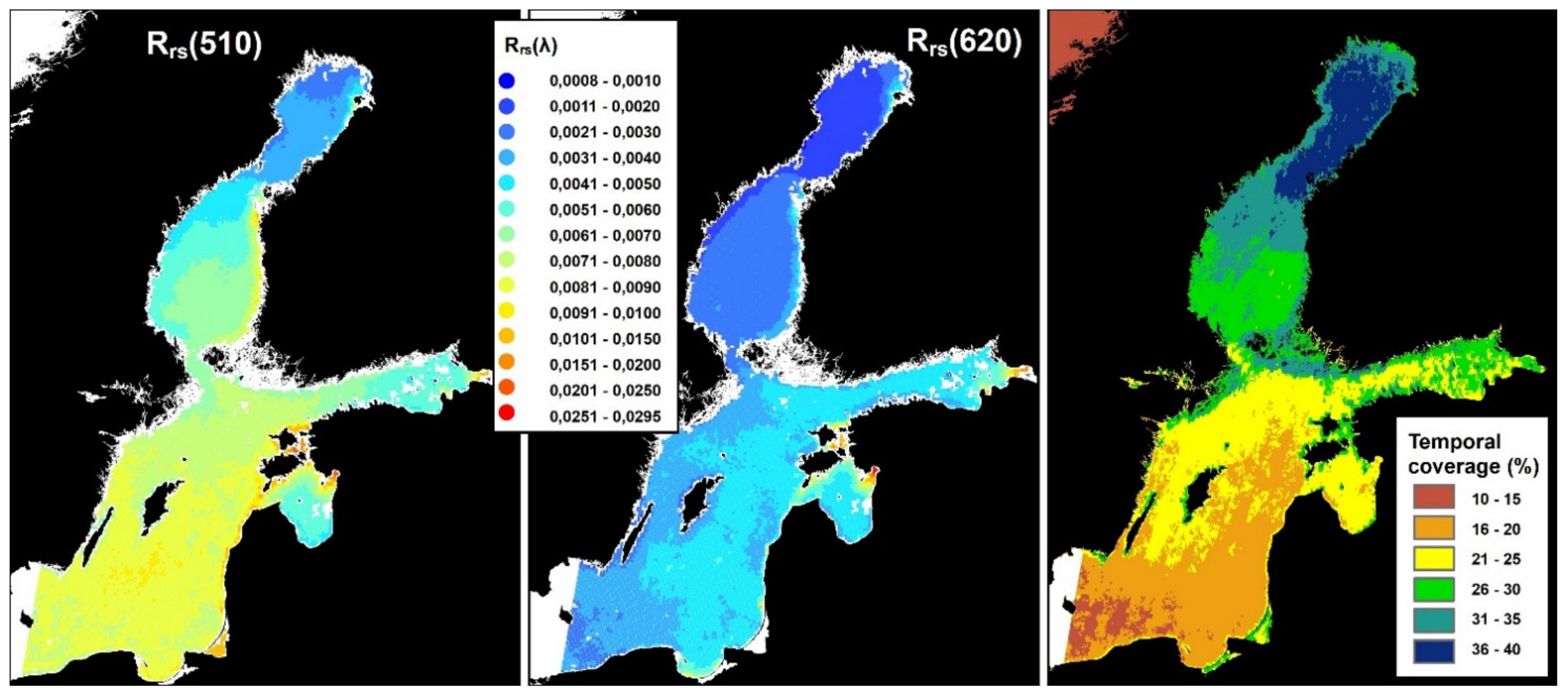
2.2. Rrs(λ) Time Series
2.3. Sampling of Rrs(λ) Data
2.4. Time Series of Physical Factors
3. Analysis Methods
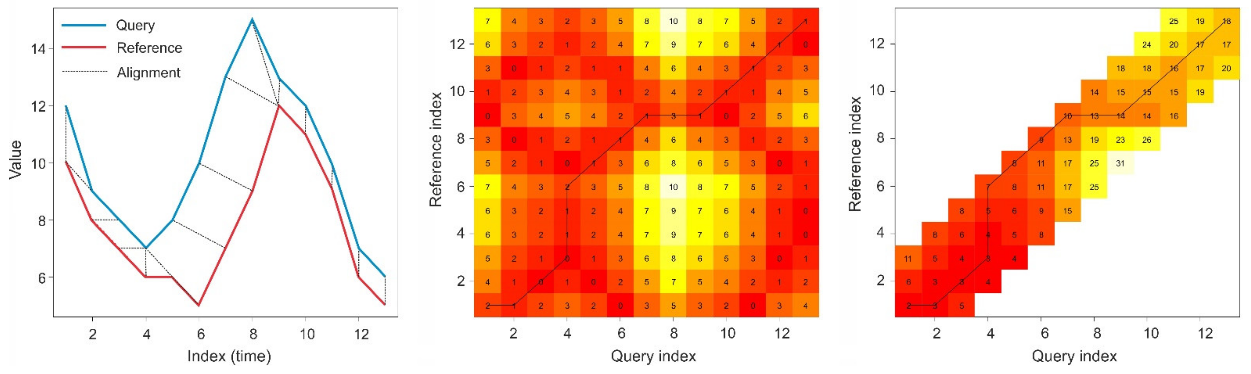
3.1. Description of Dynamic Time Warping DTW
3.2. Rationale for Selecting the Wavelengths Rrs(510) and Rrs(620)
3.3. Constructing Cost Matrix between Two Rrs(λ) Time Series by Applying DTW
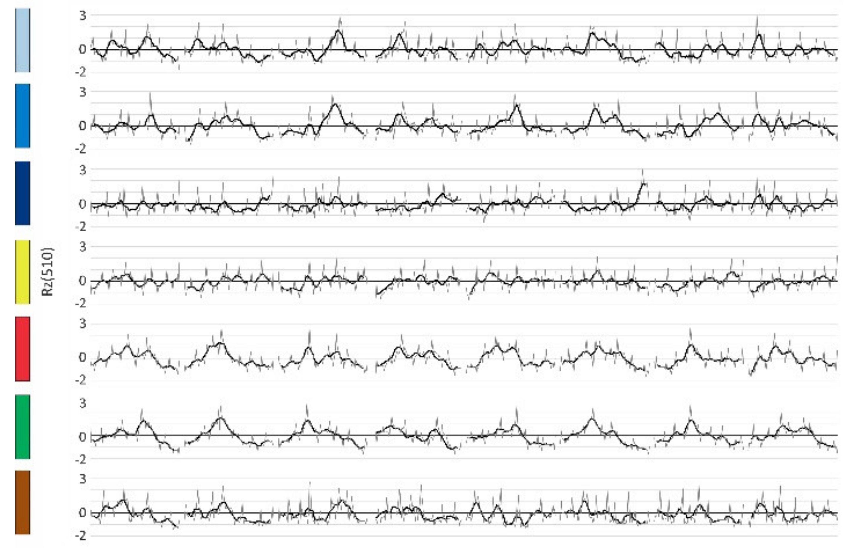
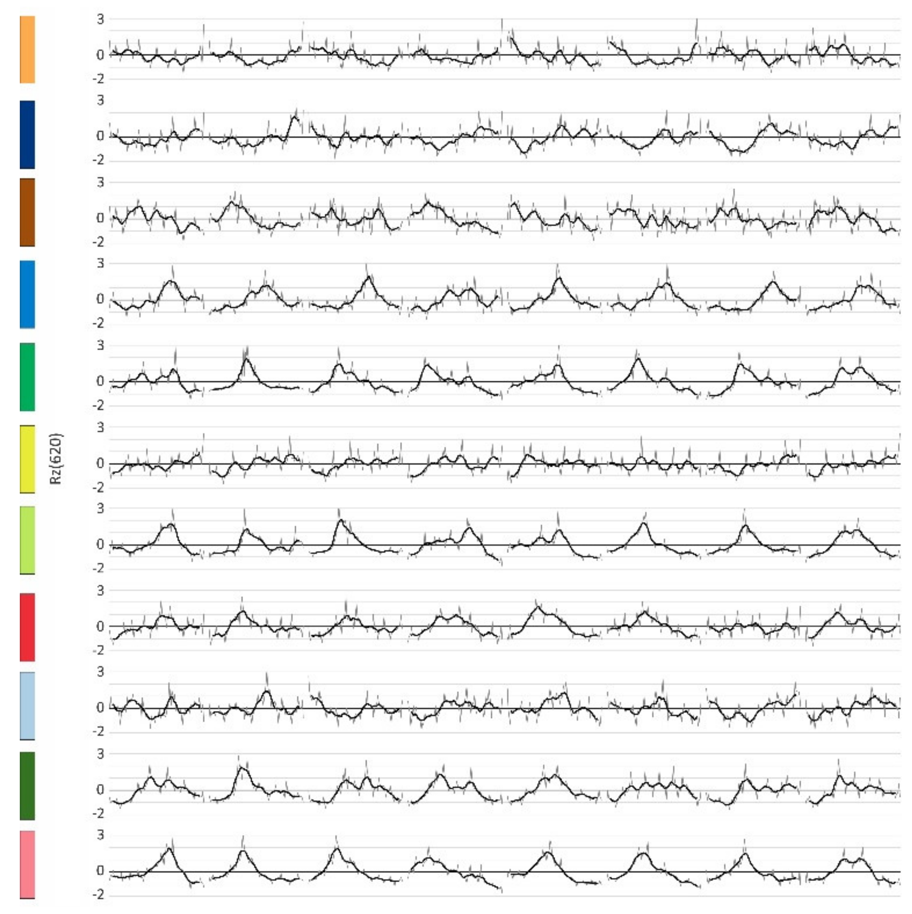
3.4. Clustering of Rz(λ) Time Series
3.5. Selecting the Value of k
3.6. Areas of Distinctive Rrs(λ) Dynamics
3.7. Relations between Physical Factors and Rz(λ)
4. Results
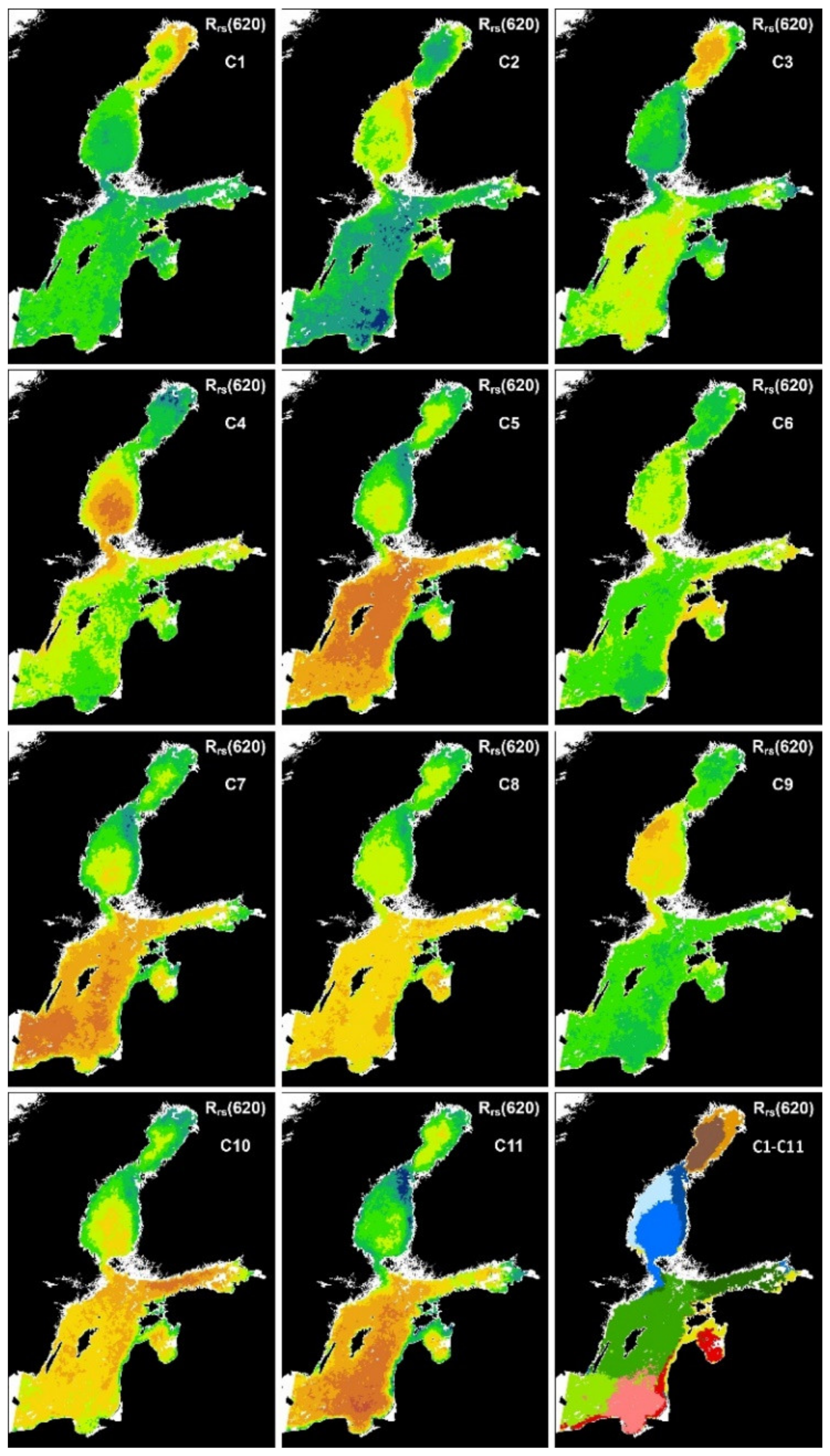
4.1. Areas of Distinctive Rrs(λ) Dynamics in Two Spectral Channels
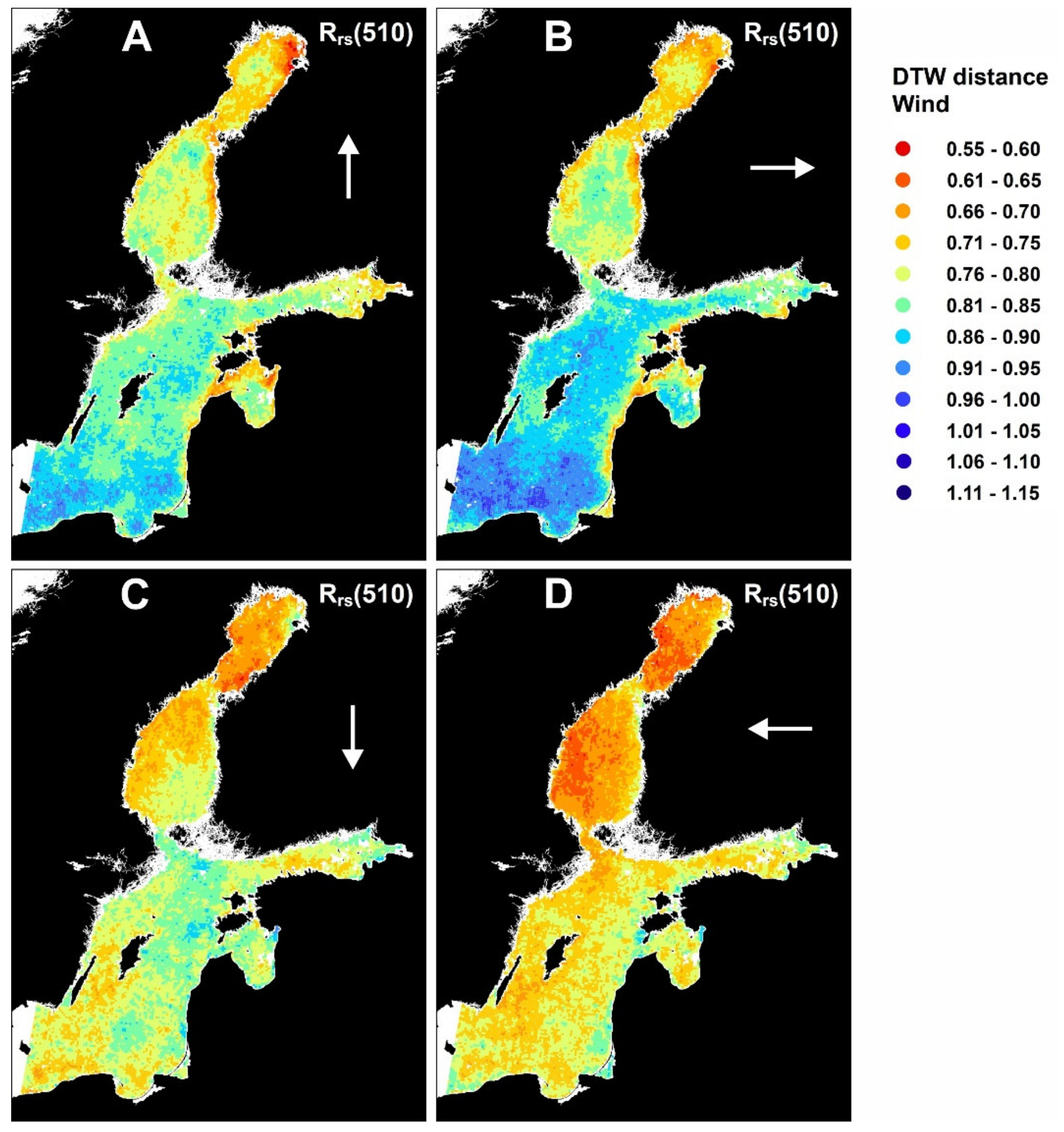
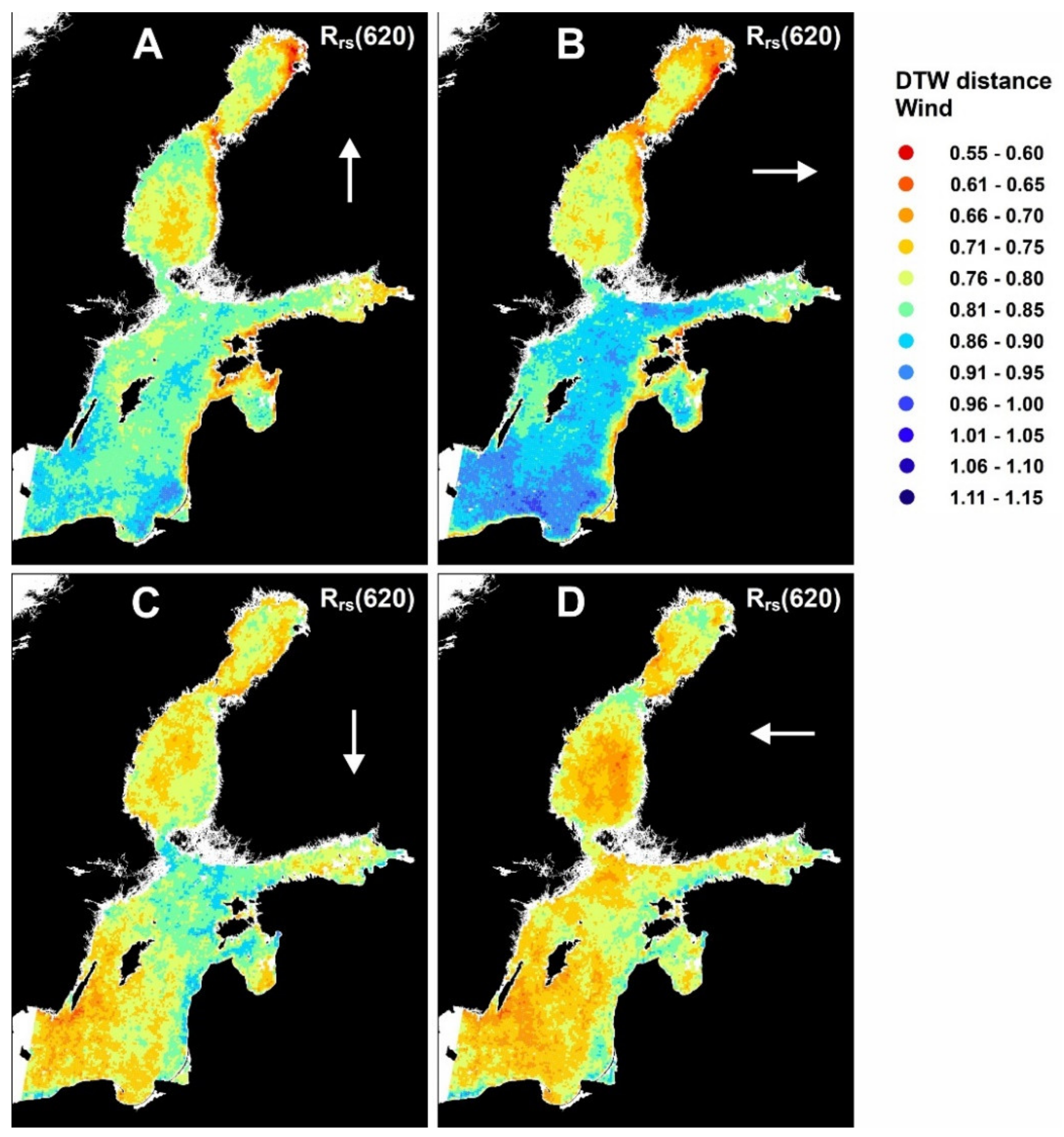
4.2. Relations between Physical Factors and Reflectance
5. Discussion
5.1. Areas of Distinctive Rrs(λ) Dynamics and Their Relations to Physical Factors
5.2. Applicability of the Proposed Workflow to Define Areas of Distinctive Rrs(λ) Dynamics
6. Conclusions
Author Contributions
Funding
Institutional Review Board Statement
Informed Consent Statement
Data Availability Statement
Acknowledgments
Conflicts of Interest
Abbreviations
| AVX | Advanced Vector Extensions |
| CCM | Cumulative Cost Matrix |
| CDOM | Colored Dissolved Organic Matter |
| CVI | Cluster Validity Index |
| CMEMS | Copernicus Marine Environment Monitoring Service |
| Dij | DTW distance matrix between time series at i and j |
| DBA | Dynamic time warping Barycentric Average |
| DTW | Dynamic Time Warping |
| EO HC | Earth Observation Hierarchical Clustering |
| k | Number of clusters |
| LCM | Local Cost Matrix |
| MERIS | Medium Resolution Imaging Spectrometer |
| NetCDF | Network Common Data Form |
| P | Observed value of the physical factor |
| Pz PC | Standardized P Partional Clustering |
| μp | Mean of P |
| σp | Standard deviation of P |
| Rrs(λ) | MERIS reflectance value at wavelength λ |
| Rz(λ) | Standardized Rrs(λ) |
| μR(λ) | Annual mean of Rrs(λ) |
| σR(λ) | Annual standard deviation of Rrs(λ) |
| s(i) | Silhouette index for time series at i |
| SPM | Suspended Particulate Matter |
| SST | Sea Surface Temperature |
| ΔSST | SST minus the median SST of five preceding days |
| ΔSSTz | Standardized ΔSST |
References
- Concha, J.; Mannino, A.; Franz, B.; Kim, W. Uncertainties in the Geostationary Ocean ColorImager (GOCI) Remote Sensing Reflectance for Assessing Diurnal Variability of Biogeochemical Processes. Remote Sens. 2019, 11, 295. [Google Scholar] [CrossRef] [Green Version]
- Karagali, I.; Høyer, J.; Hasager, C. SST diurnal variability in the North Sea and the Baltic Sea. Remote Sens. Environ. 2012, 121, 159–170. [Google Scholar] [CrossRef]
- Le Borgne, P.; Legendre, G.; Péré, S. Comparison of MSG/SEVIRI and drifting buoy derived diurnal warming estimates. Remote Sens. Environ. 2012, 124, 622–626. [Google Scholar] [CrossRef]
- Salgado-Hernanz, P.M.; Racault, M.-F.; Font-Muñoz, J.S.; Basterretxea, G. Trends in phytoplankton phenology in the Mediterranean Sea based on ocean-colour remote sensing. Remote Sens. Environ. 2019, 221, 50–64. [Google Scholar] [CrossRef]
- Simis, S.G.H.; Ylöstalo, P.; Kallio, K.; Spilling, K.; Kutser, T. Contrasting seasonality in optical-biogeochemical properties of the Baltic Sea. PLoS ONE 2017, 12, e0173357. [Google Scholar] [CrossRef]
- Ashok, K.; Yamagata, T. The El Niño with a difference. Nature 2009, 461, 481–484. [Google Scholar] [CrossRef]
- Nicholls, N. Recent trends in the seasonal and temporal behaviour of the El Niño–Southern Oscillation. Geophys. Res. Lett. 2008, 35, L19703. [Google Scholar] [CrossRef]
- Carstensen, J.; Klais, R.; Cloern, J.E. Phytoplankton blooms in estuarine and coastal waters: Seasonal patterns and key species. Estuar. Coast. Shelf Sci. 2015, 162, 98–109. [Google Scholar] [CrossRef] [Green Version]
- Fleming-Lehtinen, V.; Laamanen, M.; Kuosa, H.; Haahti, H.; Olsonen, R. Long-term development of inorganic nu-trients and chlorophyll a in the open northern Baltic Sea. Ambio 2008, 37, 86–92. [Google Scholar] [CrossRef]
- Fleming-Lehtinen, V.; Andersen, J.H.; Carstensen, J.; Łysiak-Pastuszak, E.; Murray, C.; Pyhälä, M.; Laamanen, M. Recent developments in assessment methodology reveal that the Baltic Sea eutrophication problem is expanding. Ecol. Indic. 2014, 48, 380–388. [Google Scholar] [CrossRef] [Green Version]
- Havenland, J.N. How will Ocean Acidification Affect Baltic Sea Ecosystems? An Assessment of Plausible Impacts on Key Functional Groups. Ambio 2012, 41, 637–644. [Google Scholar] [CrossRef] [PubMed] [Green Version]
- Pörtner, H.-O.; Roberts, D.C.; Masson-Delmotte, V.; Zhai, P.; Tignor, M.; Poloczanska, E.; Mintenbeck, K.; Alegría, A.; Nicolai, M.; Okem, A. (Eds.) IPCC Special Report on the Ocean and Cryosphere in a Changing Climate; IPCC: Geneva, Switzerland, 2019; in press. [Google Scholar]
- BACC (BALTEX Assessment of Climate Change for the Baltic Sea basin) Author Team. Assessment of Climate Change for the Baltic Sea Basin; Springer: Berlin/Heidelberg, Germany, 2008; 474p. [Google Scholar]
- DeFriez, E.J.; Sheppard, L.W.; Reid, P.C.; Reuman, D.C. Climate change-related regime shifts have altered spatial synchrony of plankton dynamics in the North Sea. Glob. Chang. Biol. 2016, 22, 2069–2080. [Google Scholar] [CrossRef] [PubMed] [Green Version]
- Andersen, J.H.; Axe, P.; Backer, H.; Carstensen, J.; Claussen, U.; Fleming-Lehtinen, V.; Jarvinen, M.; Kaartokallio, H.; Knuuttila, S.; Korpinen, S.; et al. Getting the measure of eutrophication in the Baltic Sea: Towards improved assessment principles and methods. Biogeochemistry 2010, 106, 137–156. [Google Scholar] [CrossRef] [Green Version]
- Leipe, T.; Moros, M.; Kotilainen, A.; Vallius, H.; Kabel, K.; Endler, M.; Kowalski, N. Mercury in Baltic Sea sediments—Natural background and anthropogenic impact. Chemistry 2013, 73, 249–259. [Google Scholar] [CrossRef]
- Deyoung, B.; Barange, M.; Beaugrand, G.; Harris, R.; Perry, R.I.; Scheffer, M.; Werner, F. Regime shifts in marine ecosystems: Detection, prediction and management. Trends Ecol. Evol. 2008, 23, 402–409. [Google Scholar] [CrossRef]
- Dippner, J.W.; Möller, C.; Hänninen, J. Regime shifts in North Sea and Baltic Sea: A comparison. J. Mar. Syst. 2012, 105–108, 115–122. [Google Scholar] [CrossRef]
- Costa, W.S.; Fonseca, L.M.G.; Körting, T.S.; do Nascimento Bendini, H.; de Souza, R.C.M. Spatio-Temporal Segmentation Applied to Optical Remote Sensing Image Time Series. IEEE Geosci. Remote Sens. Lett. 2018, 15, 1299–1304. [Google Scholar] [CrossRef]
- Jönsson, P.; Eklundh, L. TIMESAT—A program for analysing time-series of satellite sensor data. Comput. Geosci. 2004, 30, 833–845. [Google Scholar] [CrossRef] [Green Version]
- Lhermitte, S.; Verbesselt, J.; Verstraeten, W.; Coppin, P. A comparison of time series similarity measures for classification and change detection of ecosystem dynamics. Remote Sens. Environ. 2011, 115, 3129–3152. [Google Scholar] [CrossRef]
- Maus, V.; Camara, G.; Cartaxo, R.; Sanchez, A.; Ramos, F.M.; de Queiroz, G.R. A Time-Weighted Dynamic Time Warping Method for Land-Use and Land-Cover Mapping. IEEE J. Sel. Top. Appl. Earth Obs. Remote Sens. 2016, 9, 1–11. [Google Scholar] [CrossRef]
- Verbesselt, J.; Hyndman, R.; Newnham, G.; Culvenor, D. Detecting trend and seasonal changes in satellite image time series. Remote Sens. Environ. 2010, 114, 106–115. [Google Scholar] [CrossRef]
- Zhang, Y.; Hepner, G.F. The Dynamic-Time-Warping-based k-means++ clustering and its application in phenoregion delineation. Int. J. Remote Sens. 2017, 38, 1720–1736. [Google Scholar] [CrossRef]
- Reusch, T.B.H.; Boyd, P.W. Experimental Evolution Meets Marine Phytoplankton. Evolution 2013, 67, 1849–1859. [Google Scholar] [CrossRef]
- Loisel, H.; Vantrepotte, V.; Ouillon, S.; Ngoc, D.D.; Herrmann, M.; Tran, V.; Mériaux, X.; Dessailly, D.; Jamet, C.; Duhaut, T.; et al. Assessment and analysis of the chlorophyll-a concentration variability over the Vietnamese coastal waters from the MERIS ocean color sensor (2002–2012). Remote Sens. Environ. 2017, 190, 217–232. [Google Scholar] [CrossRef]
- Platt, T.; White, G.N., III; Zhai, L.; Sathyendranath, S.; Shovonlal, R. The phenology of phytoplankton blooms: Ecosystem indicators from remote sensing. Écol. Model. 2009, 220, 3057–3069. [Google Scholar] [CrossRef]
- Racault, M.-F.; Le Quéré, C.; Buitenhuis, E.; Sathyendranath, S.; Platt, T. Phytoplankton phenology in the global ocean. Ecol. Indic. 2012, 14, 152–163. [Google Scholar] [CrossRef]
- Krug, L.A.; Platt, T.; Sathyendranath, S.; Barbosa, A.B. Ocean surface partitioning strategies using ocean colour remote Sensing: A review. Prog. Oceanogr. 2017, 155, 41–53. [Google Scholar] [CrossRef]
- Dutkiewicz, S.; Beaugrand, G.; Hoepffner, N.; Kamykowski, D.; Mélin, F. Applications to biogeochemical cycles and global climate change. In Partition of the Ocean into Ecological Provinces: Role of Ocean-Colour Radiometry; Reports and Monographs of the International Ocean-Colour Coordinating Group (IOCCG); Dowell, M., Platt, T., Stuart, V., Eds.; IOCCG: Dartmouth, NS, Canada, 2009; Volume 9, pp. 47–67. [Google Scholar]
- Fay, A.R.; McKinley, G.A. Global open-ocean biomes: Mean and temporal variability. Earth Syst. Sci. Data 2014, 6, 273–284. [Google Scholar] [CrossRef] [Green Version]
- Sarmiento, J.L.; Slater, R.; Barber, R.; Bopp, L.; Doney, S.C.; Hirst, A.C.; Kleypas, J.; Matear, R.; Mikolajewicz, U.; Monfray, P.; et al. Response of ocean ecosystems to climate warming. Glob. Biogeochem. Cycles 2004, 18. [Google Scholar] [CrossRef] [Green Version]
- Nieblas, A.-E.; Drushka, K.; Reygondeau, G.; Rossi, V.; Demarcq, H.; Dubroca, L.; Bonhommeau, S. Defining Mediterranean and Black Sea Biogeochemical Subprovinces and Synthetic Ocean Indicators Using Mesoscale Oceanographic Features. PLoS ONE 2014, 9, e111251. [Google Scholar] [CrossRef] [PubMed] [Green Version]
- Mélin, F.; Vantrepotte, V. How optically diverse is the coastal ocean? Remote Sens. Environ. 2015, 160, 235–251. [Google Scholar] [CrossRef]
- Trochta, J.T.; Mouw, C.B.; Moore, T.S. Remote sensing of physical cycles in Lake Superior using a spatio-temporal analysis of optical water typologies. Remote Sens. Environ. 2015, 171, 149–161. [Google Scholar] [CrossRef]
- Gregr, E.J.; Ahrens, A.L.; Perry, R.I. Reconciling classifications of ecologically and biologically significant areas in the world’s oceans. Mar. Policy 2012, 36, 716–726. [Google Scholar] [CrossRef]
- Roff, J.C.; Taylor, M.E.; Laughren, J. Geophysical approaches to the classification, delineation and monitoring of marine habitats and their communities. Aquat. Conserv. Mar. Freshw. Ecosyst. 2003, 13, 77–90. [Google Scholar] [CrossRef]
- Suominen, T. Applying MERIS time series and dynamic time warping for delineating areas with similar temporal behaviour in the northern Baltic Sea. Ecol. Indic. 2018, 95, 794–804. [Google Scholar] [CrossRef]
- Mantas, V.; Pereira, A.; Marques, J. Partitioning the ocean using dense time series of Earth Observation data. Regions and natural boundaries in the Western Iberian Peninsula. Ecol. Indic. 2019, 103, 9–21. [Google Scholar] [CrossRef]
- Aghabozorgi, S.; Shirkhorshidi, A.S.; Wah, T.Y. Time-series clustering—A decade review. Inf. Syst. 2015, 53, 16–38. [Google Scholar] [CrossRef]
- Serrà, J.; Arcos, J.L. An empirical evaluation of similarity measures for time series classification. Knowl. Based Syst. 2014, 67, 305–314. [Google Scholar] [CrossRef] [Green Version]
- Sakoe, E.; Chiba, S. Dynamic programming algorithm optimization for spoken word recognition. IEEE Trans. Acoust. Speech Signal Process. 1978, 26, 43–49. [Google Scholar] [CrossRef] [Green Version]
- Belgiu, M.; Csillik, O. Sentinel-2 cropland mapping using pixel-based and object-based time-weighted dynamic time warping analysis. Remote Sens. Environ. 2018, 204, 509–523. [Google Scholar] [CrossRef]
- Petitjean, F.; Ketterlin, A.; Gançarski, P. A global averaging method for dynamic time warping, with applications to clustering. Pattern Recognit. 2011, 44, 678–693. [Google Scholar] [CrossRef]
- Bonsdorff, E.; Rönnberg, C.; Aarnio, K. Some ecological properties in relation to eutrophication in the Baltic Sea. Hydrobiologia 2002, 475, 371–377. [Google Scholar] [CrossRef]
- Korpinen, S.; Meski, L.; Andersen, J.H.; Laamanen, M. Human pressures and their potential impact on the Baltic Sea ecosystem. Ecol. Indic. 2012, 15, 105–114. [Google Scholar] [CrossRef]
- Palmén, E. Untersuchungen über die Strömungen in den Finnland umgebenden Meeren. Investigations of currents in the seas surrounding Finland. Comment. Phys. Math. Soc. Sci. Fenn. 1930, 12, 93. (In German) [Google Scholar]
- HELCOM (Helsinki Commission). Eutrophication in the Baltic Sea—An Integrated Thematic Assessment of the Effects of Nutrient Enrichment and Eutrophication in the Baltic Sea Region; Baltic Sea Environment Proceedings 115B; HELCOM: Helsinki, Finland, 2009. [Google Scholar]
- HELCOM (Helsinki Commission). Climate Change in the Baltic Sea Area: HELCOM Thematic Assessment in 2013; Baltic Sea Environment Proceedings 137; HELCOM: Helsinki, Finland, 2013. [Google Scholar]
- HELCOM (Helsinki Commission). State of the Baltic Sea—Second HELCOM Holistic Assessment 2011–2016; Baltic Sea Environment Proceedings 155; HELCOM: Helsinki, Finland, 2018. [Google Scholar]
- Anttila, S.; Fleming-Lehtinen, V.; Attila, J.; Junttila, S.; Alasalmi, H.; Hällfors, H.; Kervinen, M.; Koponen, S. A novel cyanobacterial surface accumulation indicator for the Baltic Sea. A novel earth observation based ecological indicator for cy-anobacterial blooms. Int. J Appl. Earth Obs. Geoinf. 2018, 64, 145–155. [Google Scholar] [CrossRef]
- Kahru, M.; Savchuk, O.; Elmgren, R. Satellite measurements of cyanobacterial bloom frequency in the Baltic Sea: Interannual and spatial variability. Mar. Ecol. Prog. Ser. 2007, 343, 15–23. [Google Scholar] [CrossRef]
- Rantajärvi, E.; Olsonen, R.; Hällfors, S.; Leppänen, J.-M.; Raateoja, M. Effect of sampling frequency on detection of natural variability in phytoplankton: Unattended high-frequency measurements on board ferries in the Baltic Sea. ICES J. Mar. Sci. 1998, 55, 697–704. [Google Scholar] [CrossRef] [Green Version]
- Attila, J.; Koponen, S.; Kallio, K.; Lindfors, A.; Kaitala, S.; Ylöstalo, P. MERIS Case II water processor comparison on coastal sites of the northern Baltic Sea. Remote Sens. Environ. 2013, 128, 138–149. [Google Scholar] [CrossRef]
- Kratzer, S.; Brockmann, C.; Moore, G. Using MERIS full resolution data to monitor coastal waters—A case study from Himmerfjärden, a fjord-like bay in the northwestern Baltic Sea. Remote Sens. Environ. 2008, 112, 2284–2300. [Google Scholar] [CrossRef]
- Kratzer, S.; Kyryliuk, D.; Brockmann, C. Inorganic suspended matter as an indicator of terrestrial influence in Baltic Sea coastal areas—Algorithm development and validation, and ecological relevance. Remote Sens. Environ. 2020, 237, 111609. [Google Scholar] [CrossRef]
- Kratzer, S.; Tett, P. Using bio-optics to investigate the extent of coastal waters: A Swedish case study. Hydrobiology 2009, 629, 169–186. [Google Scholar] [CrossRef]
- Copernicus—Marine Environment Monitoring Service. Available online: https://marine.copernicus.eu/ (accessed on 15 January 2020).
- Doxaran, D.; Bustamante, J.; Dogliotti, A.I.; Malthus, T.J.; Senechal, N. Editorial for the Special Issue “Remote Sensing in Coastal Zone Monitoring and Management—How Can Remote Sensing Challenge the Broad Spectrum of Temporal and Spatial Scales in Coastal Zone Dynamic?”. Remote Sens. 2019, 11, 1028. [Google Scholar] [CrossRef] [Green Version]
- Kratzer, S.; Harvey, E.T.; Philipson, P. The use of ocean color remote sensing in integrated coastal zone manage-ment-A case study from Himmerfjärden, Sweden. Mar. Policy 2014, 43, 29–39. [Google Scholar] [CrossRef]
- Beltrán-Abaunza, J.M.; Kratzer, S.; Brockmann, C. Evaluation of MERIS products from Baltic Sea coastal waters rich in CDOM. Ocean Sci. 2014, 10, 377–396. [Google Scholar] [CrossRef] [Green Version]
- Toming, K.; Kutser, T.; Uiboupin, R.; Arikas, A.; Vahter, K.; Paavel, B. Mapping Water Quality Parameters with Sentinel-3 Ocean and Land Colour Instrument imagery in the Baltic Sea. Remote Sens. 2017, 9, 1070. [Google Scholar] [CrossRef] [Green Version]
- Attila, J.; Kauppila, P.; Kallio, K.Y.; Alasalmi, H.; Keto, V.; Bruun, E.; Koponen, S. Applicability of Earth Observation chlorophyll-a data in assessment of water status via MERIS—With implications for the use of OLCI sensors. Remote Sens. Environ. 2018, 212, 273–287. [Google Scholar] [CrossRef]
- Doerffer, R.; Schiller, H. The MERIS Case 2 algorithm. Int. J. Remote Sens. 2007, 28, 517–535. [Google Scholar] [CrossRef]
- Doerffer, R.; Schiller, H. MERIS Regional Coastal and Lake Case 2 Water Project Atmospheric Correction ATBD (Algorithm Theoretical Basis Document) 1.0.; GKSS Forschungszentrum Geesthacht GmbH: Geesthacht, Germany, 2008; 42p. [Google Scholar]
- Doerffer, R.; Schiller, H. Lake Water Algorithm for BEAM ATBD (Algorithm Theoretical Basis Document). 1.0.; GKSS Forschungszentrum Geesthacht GmbH: Geesthacht, Germany, 2008; 17p. [Google Scholar]
- Copernicus. 2021. Available online: http://marine.copernicus.eu/documents/PUM/CMEMS-OC-PUM-009-ALL.pdf (accessed on 3 March 2021).
- Campbell, J.W.; Blaisdell, J.M.; Darzi, M. Level-3 SeaWiFS Data Products: Spatial and Temporal Binning Algorithms; Hooker, S.B., Firestone, E.R., Acker, J.G., Eds.; NASA Technical Memorandum 104566; NASA Goddard Space Flight Center: Greenbelt, MD, USA, 1995; Volume 32. [Google Scholar]
- SNAP. 2021. Available online: https://step.esa.int/main/toolboxes/snap/ (accessed on 3 March 2021).
- Bazile, E.R.; Abida, A.; Verelle, P.; Le Moigne, C.S. MESCAN-SURFEX Surface Analysis, Deliverable D2.8 of the UERRA Project. 2017. Available online: http://www.uerra.eu/publications/deliverable-reports.html (accessed on 4 October 2019).
- Copernicus. 2019. Available online: https://www.ecmwf.int/en/forecasts/datasets (accessed on 10 November 2019).
- Good, S.; Fiedler, E.; Mao, C.; Martin, M.J.; Maycock, A.; Reid, R.; Roberts-Jones, J.; Searle, T.; Waters, J.; While, J.; et al. The Current Configuration of the OSTIA System for Operational Production of Foundation Sea Surface Temperature and Ice Concentration Analyses. Remote Sens. 2020, 12, 720. [Google Scholar] [CrossRef] [Green Version]
- Merchant, C.J.; Embury, O.; Bulgin, C.E.; Block, T.; Corlett, G.K.; Fiedler, E.; Good, S.A.; Mittaz, J.; Rayner, N.A.; Berry, D.; et al. Satellite-based time-series of sea-surface temperature since 1981 for climate applications. Sci. Data 2019, 6, 1–18. [Google Scholar] [CrossRef] [Green Version]
- Copernicus. 2020. Available online: https://marine.copernicus.eu/access-data (accessed on 10 February 2020).
- Giorgino, T. Computing and Visualizing Dynamic Time Warping Alignments in R. The dtw Package. J. Stat. Softw. 2009, 31, 1–24. [Google Scholar] [CrossRef] [Green Version]
- Keogh, E.; Ratanamahatana, C.A. Exact indexing of dynamic time warping. Knowl. Inf. Syst. 2005, 7, 358–386. [Google Scholar] [CrossRef]
- Gordon, H.R.; Brown, O.B.; Evans, R.H.; Brown, J.W.; Smith, R.C.; Baker, K.S.; Clark, D.K. A semianalytic radiance model of ocean color. J. Geophys. Res. Space Phys. 1988, 93, 10909–10924. [Google Scholar] [CrossRef]
- Gordon, H.; Wang, M. Retrieval of water-leaving radiance and aerosol optical thickness over the oceans with Sea-WiFS: A preliminary algorithm. Appl. Opt. 1994, 33, 443–452. [Google Scholar] [CrossRef]
- Kratzer, S.; Vinterhav, C. Improvement of MERIS level 2 products in Baltic Sea coastal areas by applying the Improved Contrast between Ocean and Land processor (ICOL)—Data analysis and validation. Oceanologia 2010, 52, 211–236. [Google Scholar] [CrossRef]
- Needleman, S.B.; Wunsch, C.D. A general method applicable to the search for similarities in the amino acid sequence of two proteins. J. Mol. Biol. 1970, 48, 443–453. [Google Scholar] [CrossRef]
- Sardá-Espinosa, A. Time-Series Clustering in R Using the dtwclust Package. R J. 2019, 11, 22–43. [Google Scholar] [CrossRef]
- Rousseeuw, P.J. Silhouettes: A graphical aid to the interpretation and validation of cluster analysis. J. Comput. Appl. Math. 1987, 20, 53–65. [Google Scholar] [CrossRef] [Green Version]
- Pebesma, E. Simple Features for R: Standardized Support for Spatial Vector Data. R J. 2018, 10, 439–446. [Google Scholar] [CrossRef] [Green Version]
- Hijmans, R.J. Geosphere: Spherical Trigonometry. R Package Version 1.5–10. 2019. Available online: https://CRAN.R-project.org/package=geosphere (accessed on 15 November 2019).
- Hijmans, R.J. Raster: Geographic Data Analysis and Modeling. Available online: https://CRAN.R-project.org/package=raster (accessed on 15 November 2019).
- Pierce, D. ncdf4: Interface to Unidata netCDF (Version 4 or Earlier) Format Data Files. R package version 1.17. 2019. Available online: https://CRAN.R-project.org/package=ncdf4 (accessed on 5 November 2019).
- Bivand, R.; Keitt, T.; Rowlingson, B. rgdal: Bindings for the ‘Geospatial’ Data Abstraction Library. R Package Version 1.4–8. 2019. Available online: https://CRAN.R-project.org/package=rgdal (accessed on 10 January 2020).
- Kratzer, S.; Moore, G. Inherent Optical Properties of the Baltic Sea in Comparison to Other Seas and Oceans. Remote Sens. 2018, 10, 418. [Google Scholar] [CrossRef] [Green Version]
- Pettersson, C.; Allard, B.; Borén, H. River Discharge of Humic Substances and Humic-bound Metals to the Gulf of Bothnia. Estuar. Coast. Shelf Sci. 1997, 44, 533–541. [Google Scholar] [CrossRef]
- Berthon, J.-F.; Zibordi, G. Optically black waters in the northern Baltic Sea. Geophys. Res. Lett. 2010, 37. [Google Scholar] [CrossRef]
- Nausch, M.; Nausch, G.; Lass, H.U.; Mohrholz, V.; Nagel, K.; Siegel, H.; Wasmund, N. Phosphorus input by upwelling in the eastern Gotland Basin (Baltic Sea) in summer and its effects on filamentous cyanobacteria. Estuar. Coast. Shelf Sci. 2009, 83, 434–442. [Google Scholar] [CrossRef]
- Vahtera, E.; Laanemets, J.; Pavelson, J.; Huttunen, M.; Kononen, K. Effect of upwelling on the pelagic environment and bloom-forming cyanobacteria in the western Gulf of Finland, Baltic Sea. J. Mar. Syst. 2005, 58, 67–82. [Google Scholar] [CrossRef]
- Carstensen, J.; Frohn, L.M.; Hasager, C.B.; Gustafsson, B.G. Summer algal blooms in a coastal ecosystem: The role of atmospheric deposition versus entrainment fluxes. Estuar. Coast. Shelf Sci. 2005, 62, 595–608. [Google Scholar] [CrossRef]
- Radziejewska, T.; Kotta, J.; Kotwicki, L. Sandy coasts. In Biological Oceanography of the Baltic Sea; Snoeijs-Leijonmalm, P., Schubert, H., Radziejewska, T., Eds.; Springer: Berlin/Heidelberg, Germany, 2017; 683p. [Google Scholar]
- Dabuleviciene, T.; Kozlov, I.E.; Vaiciute, D.; Dailidiene, I. Remote Sensing of Coastal Upwelling in theSouth-Eastern Baltic Sea: Statistical Properties and Implications for the Coastal Environment. Remote Sens. 2018, 10, 1752. [Google Scholar] [CrossRef] [Green Version]
- Kuhrts, C.; Fennel, W.; Seifert, T. Model studies of transport of sedimentary material in the western Baltic. J. Mar. Syst. 2004, 52, 167–190. [Google Scholar] [CrossRef]


| Rrs(443) | Rrs(510) | Rrs(620) | Rz(443) | Rz(510) | Rz(620) | |||
|---|---|---|---|---|---|---|---|---|
| Rrs(510) | 0.92 | Rz(510) | 0.94 | |||||
| Rrs(620) | 0.45 | 0.68 | Rz(620) | 0.46 | 0.67 | |||
| Rrs(665) | 0.38 | 0.61 | 0.99 | Rz(665) | 0.36 | 0.58 | 0.99 |
| Cluster ID | k = 12 | k = 11 | k = 10 | k = 9 | k = 8 | k = 7 | k = 6 |
| Total mean | 0.11 | 0.10 | 0.10 | 0.11 | 0.11 | 0.13 | 0.11 |
| C1 | 0.1 | 0.17 | 0.11 | 0.12 | 0.18 | 0.09 | 0.18 |
| C2 | 0.08 | 0.18 | 0.18 | 0.08 | 0.10 | 0.16 | 0.11 |
| C3 | 0.13 | 0.08 | 0.03 | 0.08 | 0.12 | 0.12 | 0.01 |
| C4 | 0.15 | 0.11 | 0.10 | 0.12 | 0.05 | 0.02 | 0.11 |
| C5 | 0.08 | 0.08 | 0.22 | 0.22 | 0.10 | 0.06 | 0.10 |
| C6 | 0.21 | 0.22 | 0.16 | 0.15 | 0.13 | 0.16 | 0.12 |
| C7 | 0.13 | 0.15 | 0.08 | 0.09 | 0.02 | 0.15 | |
| C8 | 0.11 | 0.07 | 0.10 | 0.13 | 0.09 | ||
| C9 | 0.17 | 0.07 | 0.08 | 0.03 | |||
| C10 | 0.06 | 0.02 | 0.08 | ||||
| C11 | 0.11 | 0.10 | |||||
| C12 | 0.03 | ||||||
| Cluster ID | k = 12 | k = 11 | k = 10 | k = 9 | k = 8 | k = 7 | k = 6 |
| Total mean | 0.13 | 0.14 | 0.14 | 0.14 | 0.14 | 0.18 | 0.20 |
| C1 | 0.16 | 0.16 | 0.14 | 0.11 | 0.19 | 0.19 | 0.16 |
| C2 | 0.20 | 0.18 | 0.10 | 0.20 | 0.09 | 0.13 | 0.11 |
| C3 | 0.18 | 0.18 | 0.20 | 0.17 | 0.25 | 0.19 | 0.24 |
| C4 | 0.12 | 0.26 | 0.25 | 0.25 | 0.14 | 0.23 | 0.26 |
| C5 | 0.22 | 0.11 | 0.13 | 0.15 | 0.06 | 0.11 | 0.07 |
| C6 | 0.13 | 0.07 | 0.13 | 0.06 | 0.18 | 0.07 | 0.07 |
| C7 | 0.13 | 0.15 | −0.01 | 0.05 | 0.07 | 0.00 | |
| C8 | 0.13 | −0.03 | 0.07 | 0.17 | 0.10 | ||
| C9 | 0.09 | 0.10 | 0.19 | 0.09 | |||
| C10 | 0.05 | 0.13 | 0.11 | ||||
| C11 | 0.11 | 0.18 | |||||
| C12 | −0.01 | ||||||
Publisher’s Note: MDPI stays neutral with regard to jurisdictional claims in published maps and institutional affiliations. |
© 2021 by the authors. Licensee MDPI, Basel, Switzerland. This article is an open access article distributed under the terms and conditions of the Creative Commons Attribution (CC BY) license (https://creativecommons.org/licenses/by/4.0/).
Share and Cite
Suominen, T.; Westerholm, J.; Kalliola, R.; Attila, J. Partition of Marine Environment Dynamics According to Remote Sensing Reflectance and Relations of Dynamics to Physical Factors. Remote Sens. 2021, 13, 2104. https://doi.org/10.3390/rs13112104
Suominen T, Westerholm J, Kalliola R, Attila J. Partition of Marine Environment Dynamics According to Remote Sensing Reflectance and Relations of Dynamics to Physical Factors. Remote Sensing. 2021; 13(11):2104. https://doi.org/10.3390/rs13112104
Chicago/Turabian StyleSuominen, Tapio, Jan Westerholm, Risto Kalliola, and Jenni Attila. 2021. "Partition of Marine Environment Dynamics According to Remote Sensing Reflectance and Relations of Dynamics to Physical Factors" Remote Sensing 13, no. 11: 2104. https://doi.org/10.3390/rs13112104