Observation of Diurnal Ground Surface Changes Due to Freeze-Thaw Action by Real-Time Kinematic Unmanned Aerial Vehicle

Abstract

Ground surface changes caused by freeze-thaw action affect agriculture and forestry, as well as artificial structures such as roads. In this study, an area is examined in which reforestation is urgently needed but the growth of naturally restored seedlings and planted trees is impaired by freeze-thaw action. Thus, a method of measuring freeze-thaw induced ground surface changes and mitigating their negative impacts is needed. Real-time kinematic unmanned aerial vehicle and structure-from-motion multiview stereophotogrammetry are used on slope-failure sites in forest areas to observe the ground surface changes caused by freeze-thaw action over a wide area, in a nondestructive manner. The slope characteristics influencing the ground-surface changes were examined, and it was confirmed that it is possible to observe minute topographical changes of less than ±5 cm resulting from freeze-thaw action. Statistical models show that the amount of freeze-thaw action is mostly linked to the cumulative solar radiation, daily ground-surface temperature range, and topographic-wetness index, which influence the microscale dynamics of the ground surface. The proposed method will be useful for future quantitative assessments of ground-surface conditions. Further, efficient reforestation could be implemented by considering the effects of the factors identified on the amount of freeze-thaw action.

1. Introduction

Freeze-thaw action of soil occurs worldwide wherever the minimum temperature is below 0 °C, and it is especially noticeable in soils that are highly susceptible to frost heaving, such as volcanic-ash and peat layers. Freeze-thaw action can negatively affect human activity. In agriculture and forestry, it reportedly inhibits water flow and can cut plant roots, resulting in lodging [1]. Freeze-thaw action also damages artificial structures such as roads [2]. The frequency and intensity of freeze-thaw cycles can show a heterogeneous spatial distribution on a small scale (e.g., microtopography) depending on the environmental conditions [3]. Therefore, quantifying the spatial distribution of freeze-thaw action is essential to mitigating its negative impacts on human activities.

Traditionally, the erosion-pin method has been used to measure the ground-surface changes caused by freeze-thaw action. In this method, many pins are pierced into the ground, and the ground altitude of each pin is measured [4,5]. However, this method has limitations in terms of capturing detailed and/or accurate ground-surface changes. In this method, if the erosion pin is not deeply inserted into stable ground, it may be lifted by frost heaving. In addition, the microtopography could be disturbed by the investigators during the installation or measurement of the erosion pins. This method is also restricted in terms of the scale of measurement (e.g., point [6] and quadrat [7]). To measure more accurately the ground-surface changes caused by freeze-thaw action over a wider area, a new measurement method should be developed.

In recent years, there has been remarkable progress in technology for measuring detailed ground-surface change using proximity sensing, unmanned aerial vehicles (UAVs) to conduct structure-from-motion multiview stereo (SfM-MVS) photogrammetry [8,9], UAV-Lidar surveys [10,11], and terrestrial laser scanning (TLS) [2,12]. These measurement methods have spatial resolutions of several millimeters to several centimeters and can be used to measure ground surface changes easily over a wide area (several hundred square meters or more). UAV SfM-MVS systems have the lowest initial cost among these methods, at 1/5 to 1/10 of the cost of TLS and UAV-Lidar systems. UAVs that integrate real-time kinematic (RTK)–global navigation satellite systems with a positioning accuracy of several centimeters have recently become widely available. Therefore, a measurement system that combines RTK-UAV and SfM-MVS would be an excellent tool for measuring ground-surface changes in terms of cost and measurement accuracy. However, no studies have assessed the suitability of a combined RTK-UAV and SfM-MVS system for quantifying the spatial distribution of freeze-thaw action.

Understanding the relationship between freeze-thaw induced ground surface changes and topographical characteristics can contribute to the development of applied sciences such as civil engineering, agriculture, and forestry and fundamental sciences such as geomorphology and soil science. Previous studies have examined the topographical factors of ground-surface change (solifluction) associated with freeze-thaw action (e.g., [3]). However, these studies generally examined a limited number of observation sites and used methods that disturbed the terrain (e.g., the conventional erosion-pin method).

In Atsuma Town, Hokkaido, approximately 6000 collapsed areas formed as a result of the Eastern Iburi Earthquake on September 6, 2018 [13]. In this area, the dominant subsurface geology is volcanic-ash soil. Forestry once flourished in this area, but because of the earthquake, forest restoration in the area is required. However, this area is covered with thick volcanic-ash deposits, and the growth of naturally restored seedlings and planted trees have consequently been impaired by the freeze-thaw action of the soil. Ground-surface changes resulting from freeze-thaw action occur on daily, seasonal, and annual time scales. The longer the time scale, the greater the influence of other erosion factors (e.g., rill and gully erosion). Therefore, focusing on daily changes enables the effects of freeze-thaw action on ground-surface changes to be captured. The purposes of this study were (1) to verify whether the ground-surface changes caused by daily freeze-thaw action can be observed non-destructively and over a wide area, using RTK-UAV and SfM-MVS methods, and (2) to clarify the relationships between surface changes and slope characteristics.

2. Material and Methods

2.1. Study Site

This study targeted two slope-failure sites in Atsuma Town, Hokkaido (Figure 1a). Atsuma Town has an average annual temperature of 6.7 °C and annual precipitation of 1014 mm, and it is situated in a cool temperate zone [14]. In this area, Zhang et al. [15] reported 5625 collapsed areas within 46.3 km², with an average area of 8238 m² (between 100 and 10,000 m², which accounts for 75.6% of the total occurrence) and a slope angle of 15°–35°. The two slope-failure sites were located on the north side of the disaster area (Figure 1a). Slope-failure site 1 has an area of 4178 m² and an average slope of approximately 27° and faces southeast to southwest (Figure 1b). Slope-failure site 2 has an area of 2858 m² and an average slope of approximately 25° and faces northwest to northeast (Figure 1b). The surfaces of the slope-failure sites were composed of volcanic-ash soil.

Two temperature data loggers (CTD-TR-52i, T & D Co., Ltd., Nagano, Japan) were installed at a height of 1.5 m at each slope-failure site to measure the air temperature (Figure 1b). The measurement interval was 10 min. The survey was conducted from December 1, 2019, to May 12, 2020.

2.2. Field Survey

Aerial photographs were taken using two RTK-UAVs. A DJI Phantom4RTK (hereafter referred to as P4R) was utilized to measure the ground-surface changes (

Table 1. General information related to the unmanned aerial vehicle (UAV) and cameras.

UAV
Airplane model	DJI Phantom4RTK	DJI Matrice210RTK
Airplane type	Rotary-wing aircraft	Rotary-wing aircraft
Airplane weight	1391 g	4910 g
Max. duration of flight	30 min	33 min
Base station model	DJI D-RTK2	DJI D-RTK2
Cameras
Camera model	DJI FC6310R	DJI Zenmuse XT2
Number of pixels	20 M	12 M
Sensor size	5472 × 3648	640 × 512
Focal length	8.8 mm	5.0 mm

). A DJI Matrice210RTK (hereafter referred to as M210R) and thermal camera (DJI Zenmuse XT2) were employed to measure the ground-surface temperature (Table 1). Three surveys were conducted at the same area, from 15:00 to 16:00 on April 2, from 08:00 to 09:00 on April 3, and from 15:00 to 16:00 on April 3 2020 (hereafter referred to as 4/2 p.m., 4/3 a.m., and 4/3 p.m., respectively). During the surveys, the weather was cloudy on April 2 and sunny on April 3. The wind speed was less than 1 m/s on both days. The P4R surveys were conducted with a shooting altitude of 130 m, a ground-sampling distance of 3.56 cm/pix, a shutter interval of 2 s, an overlap rate of 80%, and a side-wrap rate of 80%. The M210R surveys were conducted with a shooting altitude of 150 m, a ground-sampling distance of 18.75 cm/pix, a shutter interval of 2 s, an overlap rate of 90%, and a side-wrap rate of 90%. The lap ratio of M210R was set higher than the lap ratio of P4R because thermal images generally have lower resolutions than optical images. Both UAVs can obtain aerial images using the RTK positioning method. The reference station used for RTK positioning was a DJI D-RTK2. The coordinate values of the reference station were obtained using the post-processing kinematic method, and a ProMark 120 (Spectra Precision Inc., Dayton, USA) was utilized for positioning. The angle of the UAV camera was set vertically downward. The DJI GSRTK app was employed to set the flight path and autonomous flight of the P4R, whereas the DJI GSPRO app was used to set those of the M210R.

2.3. Data Analysis

All UAV images used in the analysis had the RTK Fix solution. Metashape Professional Version 1.6.3 (Agisoft LCC, Saint Petersburg, Russia) was utilized to analyze the UAV images. This software can restore a three-dimensional shape from multiple photographs using the principle of photogrammetry. In addition, digital surface models (DSMs) and ortho-mosaic images were created. The SfM-MVS algorithm was used for this series of analyses. The camera calibration parameters, such as the focal length of the lens, were the factory defaults recorded on each UAV. A thermal map (TM) was created using the thermal images acquired with the M210R, Pix4D Mapper Version 4.5.6 (Pix4D S.A., Lausanne, Switzerland), and SfM-MVS algorithm. The thermal-image camera only acquired the relative temperatures, and these values were converted into absolute values using the temperature of running water in rivers, which showed minimal changes. First, we measured the water temperatures of streams in the study area at three locations in the morning and afternoon using a water-temperature meter. Next, we calculated the difference between the observed temperature and temperature extracted from the TM. Finally, we converted the relative temperatures from the TM into absolute temperatures (in degrees Celsius), by considering the thermal difference. The daily range of ground-surface temperatures was calculated from the difference between the TMs in the morning and afternoon.

ArcGIS 10.7 (Esri Inc., Redlands, USA) was used to conduct GIS analysis. Altitude -differential analysis was performed using the Spatial Analyst tool and two-stage DSMs to extract the surface changes (freeze-thaw amount) [16]. In addition, the inclination angle, curvature, and annual amount of cumulative solar radiation, i.e., the solar radiation received by a slope in a given year, were calculated using the 4/3 p.m. DSM. The topographic wetness index (TWI) was calculated using the SAGA GIS Modules in QGIS [17] to understand the ease of collecting water. The maps of each of these calculated variables were created as raster data, which were then averaged into 0.5 m grid polygons, output to a CSV file, and used in the generalized linear models (GLMs). These maps were used in the analysis without intentionally removing snow areas, assuming that the snow cover is suppressing freeze-thaw action.

To perform differential analysis of the multiple DSMs, we first verified their accuracies in the X, Y, and Z directions by comparing the coordinates of 10 verification points (Figure 1b). These points consisted of markers placed on the ground, and their coordinate values were extracted from the 4/2 p.m., 4/3 a.m., and 4/3 p.m. DSMs. The coordinates were compared, and the error and RMSE were calculated for each verification point. The formula used to calculate the RMSE is as follows:

$$RMSE=\surd \frac{1}{n}{{\displaystyle \sum }}_{i=1}^n(y_i-y_i)$$

(1)

We performed a t-test to compare the thermal environments of the slope-failure sites. Next, we examined the environmental factors affecting the degree of freeze-thaw using GLMs with Gaussian-distribution error. The freeze-thaw amount was used as the objective variable. The explanatory variables were the daily range of ground-surface temperatures, inclination angle, curvature, annual amount of cumulative solar radiation, and TWI.

2.4. Model Selection Procedures

Based on the result of the GLM analyses, we detected influential variables according to the following procedures. We selected variables included in the top model (i.e., with a minimum value for the Akaike information criterion (AIC) as environmental factors affecting the degree of freeze-thaw. Top model selection was performed using the R package “MuMIn” [18]. Models with an AIC difference below 2 (ΔAIC < 2) can be considered to have significant support [19]. Thus, we considered the explanatory variables that were included in all equivalent models as influential predictors when multiple equivalent top models (ΔAIC < 2) were identified. All statistical analyses were performed using the statistical software R, version 4.0.0 [20].

3. Results

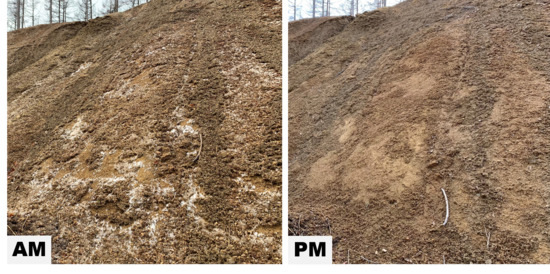
3.1. Slope-Failure Site Properties

Figure 2 shows the temperature changes at slope-failure sites 1 and 2. Figure 2a shows the temperature change during the survey period from winter to spring, and Figure 2b shows the temperature change on the survey dates from April 2 to 3, 2020. The temperature was generally higher at slope-failure site 1, where the slope was predominantly south-facing, than at slope-failure site 2, where the slope was predominantly north-facing. At 4/2 p.m., the maximum temperature was 8.4 °C and 7.3 °C at slope-failure sites 1 and 2, respectively. The temperature dropped between 4/2 p.m. to 4/3 a.m., from night to early morning, reaching −3.9 °C and −4.1 °C at slope-failure sites 1 and 2, respectively, on the morning of 4/3. The temperature was above 0 °C from around 08:00 on April 3, and the maximum temperature was 13.8 °C and 13.0 °C at slope-failure sites 1 and 2, respectively.

Figure 3 shows the UAV orthoimages on 3/13 and 4/2 p.m. On 3/13, the ground surface of slope-failure site 1 was partially exposed on the steep slope below the convex break of the slope angle, whereas slope-failure site 2 remained covered with snow. At 4/2 p.m., the ground surface at slope-failure site 1 was completely exposed on the slopes, and no snow remained, whereas at slope-failure site 2, the ground surface was exposed on more than half of the slope, but some snow remained.

3.2. Verification of DSM Accuracy Created from RTK-UAV Imagery

Table 2. Error and RMSE between the DSMs in the XYZ direction.

No.	4/2 P.M.–4/3 A.M.			4/3 P.M.–4/3 A.M.
	X	Y	Z	X	Y	Z
1	0.004	−0.069	0.078	0.005	−0.016	−0.019
2	0.039	−0.075	0.046	−0.005	−0.012	0.026
3	0.033	−0.057	0.006	−0.008	−0.011	−0.027
4	0.027	−0.068	−0.001	−0.018	−0.020	−0.039
5	0.064	−0.083	−0.001	0.025	−0.023	−0.020
6	0.036	−0.063	0.010	−0.009	−0.007	−0.009
7	0.054	−0.069	−0.063	−0.002	−0.014	−0.031
8	0.024	−0.067	−0.063	−0.011	−0.006	−0.051
9	−0.017	−0.014	−0.048	−0.015	−0.004	−0.059
10	0.019	−0.061	0.071	−0.018	−0.025	−0.010
RMSE	0.036	0.065	0.049	0.013	0.015	0.033

Unit: m.

shows the error and RMSE between the DSMs in the X, Y, and Z directions. Comparison of the DSM from 4/2 p.m. with that from 4/3 a.m. (as the true value) returned an X-, Y-, and Z-direction errors of −0.017 to 0.064 m, −0.083 to −0.014 m, and −0.063 to 0.078 m, respectively. The RMSE was 0.036 m, 0.065 m, and 0.049 m in the X-, Y-, and Z-directions, respectively.

Comparing the DSM from 4/3 p.m. with that from 4/3 a.m. (as the true value) returned X-, Y-, and Z-direction errors of −0.018 to 0.025 m, −0.025 to −0.004 m, and −0.059 to 0.026 m, respectively. The RMSE was 0.013 m, 0.015 m, and 0.033 m in the X-, Y-, and Z-directions, respectively. The Z-direction RMSE, between the DSMs used in the differential analysis, was less than ±0.05 m for both sites. Therefore, the altitude change was used in the differential analysis as a reliable value, to within 0.05 m.

3.3. Environment and Altitude Changes of the Ground Surface at Slope-Failure Sites

Figure 4 shows the annual cumulative amount of solar radiation and the daily range of ground-surface temperatures at each slope-failure site. Slope-failure site 1 had a higher annual cumulative amount of solar radiation than slope-failure site 2 (t-test, p < 0.01; Figure 4a). The daily range of ground-surface temperatures at slope-failure site 1 was also larger than that at slope-failure site 2 (t-test, p < 0.01; Figure 4b).

Figure 5 provides a map of the altitude changes. The amount of positive altitude change indicates the amount of frost heaving. Differential analysis of the DSMs from 4/2 p.m. and 4/3 a.m. confirmed that the number of cells in which the altitude of the ground-surface increased because of frost heaving was higher at slope-failure site 1 than at slope-failure site 2 (Figure 5a). The degree of altitude decrease can be interpreted by the amount of melted soil ice. Differential analysis of the DSMs from 4/3 a.m. and 4/3 p.m. confirmed that the ground-surface altitude decreased equally at the two slope-failure sites (Figure 5b). Figure 6a presents a map of the summed absolute values of frost heaving and thawing. The average amount of freeze-thaw was 0.10 ± 0.07 m and 0.08 ± 0.15 m at slope-failure sites 1 and 2, respectively. In addition, slope-failure site 1 exhibits a larger freeze-thaw amount than slope-failure site 2 (t-test, p < 0.01; Figure 6b).

3.4. Relationships among Freeze-Thaw Amount, Terrain, and the Thermal Environment

Table 3. Standardized partial regression coefficients selected in the top three models explaining the freeze-thaw amount.

Rank of Model	AIC	ΔAIC	Estimated Coefficients (Standard Error)
			Intercept	Ground Surface Temperatures	TWI	Cumulative Solar Radiation	Inclination Angle	Curvature
1	–11,297.7	0.00	0.102 *** (0.00831)	0.00106 *** (0.000130)	–0.00410 *** (0.000983)	–7.43 × 10−6 *** (1.98 × 10−6)	0.000318 (0.000167)
2	–11,296.1	1.64	0.114 *** (0.00531)	0.00113 *** (0.000126)	–0.00481 *** (0.000911)	–8.47 × 10−6 *** (1.90 × 10−6)
3	–11,295.9	1.76	0.102 *** (0.00831)	0.00106 *** (0.000130)	–0.00411 *** (0.000983)	–7.44 × 10−6 *** (1.98 × 10−6)	0.000320 (0.000167)	–2.04 × 10−7 (4.16 × 10−7)
4	–11,294.3	3.43	0.114 *** (0.00531)	0.00113 *** (0.000126)	–0.00482 *** (0. 000912)	–8.47 × 10−6 *** (1.90 × 10−6)		–1.89 × 10−7 (4.16 × 10−7)
Null model	–11,170.3	127.44	0.0923 *** (0.00130)

*** p < 0.001.

lists the details of the top four models with the lowest AICs and the null model. We detected three influential variables affecting the freeze-thaw amount: the daily range of ground-surface temperatures, TWI, and annual cumulative solar radiation. These three variables were selected in all models (ΔAIC < 2). The standardized partial regression coefficient was positive for the daily range of ground surface-temperatures, negative for TWI, and negative for the annual cumulative solar radiation, but all coefficient values were significant.

4. Discussion

4.1. Validity, Accuracy, and Applicability of DSMs Created from RTK-UAV Images

Obanawa et al. [21] verified the accuracy of DSMs created from RTK-UAV images and found errors of 0.037 to 0.327, 0.096 to 0.231 m, and 0.062 to 0.105 m in the X-, Y-, and Z-directions, respectively. The method presented here is slightly more accurate than that in the previous study, and the measurement accuracy is generally supported by the previous work. The high accuracy of the measurement may be attributed to the high overlap of DSMs. Obanawa et al. [21] set the side overlap of the images as 60%, whereas we set the overlap ratio to 80% because DSMs created from multiple images with a high overlap rate are more accurate than those created from images with a lower overlap [22]. Therefore, the constructed models showed small RMSEs in the X-, Y-, and Z-directions (0.013 to 0.065 m). In particular, the RMSE in the Z-direction was less than ±0.05 m, suggesting that ground-surface changes of ±0.05 m or more were reliable in our constructed DSMs. Previous studies conducted in the same area as this study, with the same equipment, returned RMSEs in the X-, Y-, and Z-directions of approximately 0.06 m, with a maximum error in the Z-direction of approximately 0.1 m. Nakata et al. [16] reported that it is possible to observe ground-surface changes of ±0.1 m or more. The freeze-thaw amounts detected in this previous study agreed well with our study results.

In this study, an RTK-UAV was used to create 3D surface maps. However, most previous studies have utilized UAVs without RTK positioning. DSMs constructed from UAV data, without RTK positioning, also show minor measurement errors (several centimeters), relative to ground control points (e.g., [12,23]). However, because UAVs without RTK positioning have flight accuracy inferior to that of UAVs with RTK positioning, it is necessary to set dozens of ground control points for these surveys and to provide accurate coordinates to the 3D model during analysis. Installing ground control points is relatively easy on flat terrain, such as farmlands, but installing them on slope-failure sites and collapsed land is laborious and dangerous. In addition, it has been reported that the accuracy of DSMs depends on the spatial placement of ground control points [23]. UAVs with RTK involve monetary costs about twice as high as those for UAV without RTK. However, from the perspectives of labor, safety, and versatility, the SfM-MVS method using UAVs with RTK is superior to the conventional UAV without RTK positioning.

The average amount of freeze-thaw was 0.10 ± 0.07 m and 0.08 ± 0.15 m at slope-failure sites 1 and 2, respectively. Sarsembayeva and Collins [24] observed the amount of freeze-thaw in laboratory experiments using Kazakh Steppe soils. They reported that the amounts of frost heaving and thawing were 0.05 m/day and 0.01 m/day, respectively. These results agree with those presented in this report.

4.2. Environmental Factors Affecting Freeze-thaw Amount

The annual cumulative solar radiation, daily range of ground surface temperatures, and TWI were identified as significant contributors to the three top models explaining the freeze-thaw amount (Table 3). In this study, we calculated the diurnal changes in the ground-surface altitude as the sum of the frost heaving and thawing amounts. Therefore, the freeze-thaw index reflects the effects of both freezing and thawing on ground movement. The thermal environment and water conditions of the ground are important for freeze-thaw action [25]. These variables influence the microscale dynamics of ground surfaces by regulating the thermal and hydrologic conditions of surface soils, as follows. First, the annual cumulative solar radiation negatively affects the freeze-thaw amount. Solar radiation repeatedly increases the ground-surface temperature and promotes the melting of soil ice in the long term. Thus, we assume that slopes with higher annual cumulative solar radiation generally contained less moisture at the time of our observations. As drier soils are less susceptible to freezing than wet soils, it is assumed that the freeze-thaw amount has a negative correlation with the annual cumulative solar radiation.

Second, the daily range of ground surface temperatures positively affected the freeze-thaw amount. A larger daily range of ground-surface temperatures indicates that the ground-surface temperature of the slope tends to decrease substantially during the night and then increase during the day. Nighttime low temperatures increase the frost heaving amount, while daytime high temperatures increase the frost thawing amount. Kellerer-Pirklbauer [25] highlighted the importance of the thermal environment and water condition of the ground in freeze-thaw action. This suggests that the factors affecting the surface and subsurface thermal environment, such as the daily range of ground-surface temperatures, also play important roles in freeze-thaw action.

Contrary to our expectation, the freeze-thaw amount was limited on the slope with higher TWI. In general, areas with high TWIs correspond to gullies or rill erosion areas on the slope [26,27,28]. When gully or rill erosion occurs, the surface soil is eroded, and the matrix in which soil ice growth occurs is removed. Therefore, the TWI is assumed to limit the increase in the freeze-thaw amount.

4.3. Differences in Freeze-Thaw Amount between Slope-Failure Sites

The amount of frost heaving tended to be higher at slope-failure site 1 than at slope-failure site 2, whereas the sites showed little difference in the amount of frost thawing (Figure 5). Consequently, the total amounts of frost thawing and heaving tended to be larger at slope-failure site 1 (Figure 6). In addition, the decrease in altitude at slope-failure site 2 may include decreases caused by capturing the melting of the remaining snow, resulting in a greater freeze-thaw amount at slope-failure site 1 than at slope-failure site 2. The annual cumulative solar radiation, daily range of ground-surface temperatures, TWI, and inclination angle were extracted from the best model explaining the freeze-thaw amount (Table 3). Differences in these variables between slope-failure sites may result in differences in the freeze-thaw amount.

Ice in soil begins to freeze or thaw at 0 °C [29]. From the temperature change in Figure 2, it can be inferred that on April 2, ice melted during the daytime, the temperature fell below 0 °C at approximately 22:00, and the ice stayed frozen until the morning of April 3. On the slopes on which the soil froze, it is assumed that the ground surface was lifted by frost heaving, increasing the altitude (Figure 4). On April 3, the temperature exceeded 0 °C from around 08:00, rose to 13 °C around 14:00, and did not fall below 0 °C until around 20:00. It is assumed that during that time, any soil that remained frozen continued to thaw. It is presumed that this process decreased the altitude of the ground surface.

South-facing slopes show earlier snow thawing and larger daily surface temperature ranges because they receive more solar radiation and tend to have higher surface temperatures. In addition, Kellerer-Pirklbauer [25] reported that snow covering the ground surface suppresses surface-temperature changes, resulting in decreased freeze-thaw action. Consequently, south-facing slopes generally experience larger freeze-thaw amounts than north-facing slopes [30]. On the south-facing slope at site 1, the temperature was relatively high, the snow melted quickly in early spring (Figure 2), and the daily ground-surface temperature range was large (Figure 3). These observations support the results of the previous work.

5. Conclusions

In this study, we first verified the effectiveness of a new method using an RTK-UAV and SfM-MVS algorithm to measure ground-surface changes caused by diurnal freeze-thaw action on slope-failure sites in forest areas. Furthermore, we clarified the relationships between the ground-surface changes and slope characteristics based on 3D surface maps created via this new method. We found that (1) this areawide and nondestructive method can be used to assess accurately the ground-surface changes over a wide area, with a Z-direction error of ±0.05 m, (2) the freeze-thaw amount was affected by the thermal and topological slope characteristics, and (3) the freeze-thaw amount on the south-facing slopes (slope-failure site 1) was larger than that on the north-facing slopes (slope-failure site 2).

Our study will contribute to the development of a quantitative method of assessing ground-surface conditions, such as snow-depth estimation [21], and fosters an understanding of natural phenomena. In particular, the spatiotemporal resolution improvement was remarkable. For example, in a previous study measuring ground-surface changes because of erosion and sedimentation at a slope-failure site, topographical changes of several centimeters were detected over approximately 1 month [16]. In this study, we demonstrated that the temporal resolution of surface change observations can be further improved (i.e., from half a day to one day).

Furthermore, by simultaneously examining the topographical factors that affect the freeze-thaw amount, we demonstrated the analytical applications of RTK-UAV techniques. In the study region, approximately 6000 collapsed areas formed as a result of the Hokkaido Eastern Iburi Earthquake in 2018. Rapid reforestation of slope-failure sites is urgently needed. We identified three influential factors, namely, the annual cumulative solar radiation, daily ground-surface temperature range, and TWI, which should be considered when planning efficient reforestation in this area. In the future, we will elucidate the relationship between the freeze-thaw amount/these factors and the growth of naturally restored seedlings and planted trees, which will contribute to reforestation. However, underground variables such as geological factors were not considered in this study. In the future, by mounting a microwave sensor on the RTK-UAV, it will be possible to acquire data such as that describing underground structures in a planer manner [31]. Further technological innovations and reduced sensor costs will enable the identification of other factors that influence freeze-thaw amounts in a nondestructive manner. We expect that our findings will lead to further understanding of the morphological ground-surface changes that affect ecosystems and human activities.

References

1. Saxton, K.E.; Formanek, G.E.; Molnau, M. Frozen Soil Impacts on Agricultural, Range, and Forest Land; Special Report; U.S. Army Cold Regions Research and Engineering Laboratory: Hanover, NH, USA, 1990. [Google Scholar]
2. Mill, T.; Ellmann, A.; Aavik, A.; Horemuz, M.; Sillamäe, S. Determining ranges and spatial distribution of road frost heave by terrestrial laser scanning. Balt. J. Road Bridg. Eng. 2014, 9, 225–234. [Google Scholar] [CrossRef] [Green Version]
3. Matsuoka, N. Solifluction rates, processes and landforms: A global review. Earth-Sci. Rev. 2001, 55, 107–134. [Google Scholar] [CrossRef]
4. Lawler, D.M. Needle ice processes and sediment mobilization on river banks: The River Ilston, West Glamorgan, UK. J. Hydrol. 1993, 150, 81–114. [Google Scholar] [CrossRef]
5. Couper, P.; Stott, T.; Maddock, I. Insights into river bank erosion processes derived from analysis of negative erosion-pin recordings: Observations from three recent UK studies. Earth Surf. Process. Landf. 2002, 27, 59–79. [Google Scholar] [CrossRef]
6. Matsuoka, N.; Abe, M.; Ijiri, M. Differential frost heave and sorted patterned ground: Field measurements and a laboratory experiment. Geomorphology 2003, 52, 73–85. [Google Scholar] [CrossRef]
7. Ponti, S.; Cannone, N.; Guglielmin, M. Needle ice formation, induced frost heave, and frost creep: A case study through photogrammetry at Stelvio Pass (Italian Central Alps). Catena 2018, 164, 62–70. [Google Scholar] [CrossRef]
8. Saito, H.; Uchiyama, S.; Hayakawa, Y.S.; Obanawa, H. Landslides triggered by an earthquake and heavy rainfalls at Aso volcano, Japan, detected by UAS and SfM-MVS photogrammetry. Prog. Earth Planet. Sci. 2018, 5, 1–10. [Google Scholar] [CrossRef]
9. Cook, K.L.; Dietze, M. A simple workflow for robust low-cost UAV-derived change detection without ground control points. Earth Surf. Dyn. 2019, 7, 1009–1017. [Google Scholar] [CrossRef] [Green Version]
10. Vepakomma, U.; Cormier, D. Potential of multi-temporal UAV-borne lidar in assessing effectiveness of silvicultural treatments. Int. Arch. Photogramm. Remote Sens. Spat. Inf. Sci. 2017, 42, 393–397. [Google Scholar] [CrossRef] [Green Version]
11. Sofonia, J.; Phinn, S.; Roelfsema, C.; Kendoul, F. Observing geomorphological change on an evolving coastal sand dune using SLAM-based UAV LiDAR. Remote Sens. Earth Syst. Sci. 2019, 2, 273–291. [Google Scholar] [CrossRef]
12. Neugirg, F.; Stark, M.; Kaiser, A.; Vlacilova, M.; Della Seta, M.; Vergari, F.; Schmidt, J.; Becht, M.; Haas, F. Erosion processes in calanchi in the Upper Orcia Valley, Southern Tuscany, Italy based on multitemporal high-resolution terrestrial LiDAR and UAV surveys. Geomorphology 2016, 269, 8–22. [Google Scholar] [CrossRef]
13. Osanai, N.; Yamada, T.; Hayashi, S.I.; Kastura, S.; Furuichi, T.; Yanai, S.; Murakami, Y.; Miyazaki, T.; Tanioka, Y.; Takiguchi, S.; et al. Characteristics of landslides caused by the 2018 Hokkaido Eastern Iburi Earthquake. Landslides 2019, 16, 1517–1528. [Google Scholar] [CrossRef]
14. Japan Meteorological Agency. Past Weather Data and Download. Available online: https://www.data.jma.go.jp/obd/stats/etrn/ (accessed on 20 December 2020).
15. Zhang, S.; Li, R.; Wang, F.; Iio, A. Characteristics of landslides triggered by the 2018 Hokkaido Eastern Iburi earthquake, Northern Japan. Landslides 2019, 16, 1691–1708. [Google Scholar] [CrossRef]
16. Nakata, Y.; Hayamizu, M.; Koshimizu, K.; Takeuchi, F.; Ebina, M.; Sato, H. Accuracy assessment of topographic measurements and monitoring of topographic changes using RTK-UAV in landslide area caused by 2018 Hokkaido Eastern Iburi Earthquake. Landsc. Ecol. Manag. 2020, 25, 43–52. [Google Scholar] [CrossRef]
17. QGIS Development Team. QGIS Geographic Information System. Open Source Geospatial Foundation Project. 2020. Available online: http://qgis.osgeo.org (accessed on 15 April 2020).
18. Barton, K. MuMIn: Multi-Model Inference. R Package Version 1.9.0. 2013. Available online: http://CRAN.R-project.org/package=MuMIn (accessed on 25 January 2014).
19. Burnham, K.P.; Anderson, D.R. Model Selection and Multimodel Inference: A Practical Information-Theoretic Approach; Springer: New York, NY, USA, 2013. [Google Scholar]
20. R Development Core Team. R: A Language and Environment for Statistical Computing; 2020 R (Version 4.0.0); R Development Core Team: Vienna, Austria; Available online: http://www.R-project.org (accessed on 29 April 2020).
21. Obanawa, H.; Sakanoue, S.; Yagi, T. Evaluating the Applicability of RTK-UAV for Field Management. In Proceedings of the IGARSS 2019—2019 IEEE International Geoscience and Remote Sensing Symposium, Yokahama, Japan, 28 July–2 August 2019; pp. 9090–9092. [Google Scholar]
22. Torres-Sánchez, J.; López-Granados, F.; Borra-Serrano, I.; Peña, J.M. Assessing UAV-collected image overlap influence on computation time and digital surface model accuracy in olive orchards. Precis. Agric. 2017, 19, 115–133. [Google Scholar] [CrossRef]
23. James, M.R.; Robson, S.; d’Oleire-Oltmanns, S.; Niethammer, U. Optimising UAV topographic surveys processed with structure-from-motion: Ground control quality, quantity and bundle adjustment. Geomorphology 2017, 280, 51–66. [Google Scholar] [CrossRef] [Green Version]
24. Sarsembayeva, A.; Collins, P.E.F. Evaluation of frost heave and moisture/chemical migration mechanisms in highway subsoil using a laboratory simulation method. Cold Reg. Sci. Technol. 2017, 133, 26–35. [Google Scholar] [CrossRef]
25. Kellerer-Pirklbauer, A. Potential weathering by freeze-thaw action in alpine rocks in the European Alps during a nine year monitoring period. Geomorphology 2017, 296, 113–131. [Google Scholar] [CrossRef]
26. Arabameri, A.; Blaschke, T.; Pradhan, B.; Pourghasemi, H.R.; Tiefenbacher, J.P.; Bui, D.T. Evaluation of recent advanced soft computing techniques for gully erosion susceptibility mapping: A comparative study. Sensors 2020, 20, 335. [Google Scholar] [CrossRef] [PubMed] [Green Version]
27. Arabameri, A.; Pradhan, B.; Lombardo, L. Comparative assessment using boosted regression trees, binary logistic regression, frequency ratio and numerical risk factor for gully erosion susceptibility modelling. Catena 2019, 183, 104223. [Google Scholar] [CrossRef]
28. Arabameri, A.; Chen, W.; Loche, M.; Zhao, X.; Li, Y.; Lombardo, L.; Cerda, A.; Pradhan, B.; Bui, D.T. Comparison of machine learning models for gully erosion susceptibility mapping. Geosci. Front. 2020, 11, 1609–1620. [Google Scholar] [CrossRef]
29. Konrad, J.-M.; Morgenstern, N.R. A mechanistic theory of ice lens formation in fine-grained soils. Can. Geotech. J. 1980, 17, 473–486. [Google Scholar] [CrossRef]
30. Matsuoka, N.; Hirakawa, K.; Watanabe, T.; Haeberli, W.; Keller, F. The role of diurnal, annual and millennial freeze-thaw cycles in controlling alpine slope instability. In Proceedings of the PERMAFROST—7th International Conference, Yellowknife, NT, Canada, 23–27 June 1998; pp. 711–717. [Google Scholar]
31. Schartel, M.; Burr, R.; Mayer, W.; Docci, N.; Waldschmidt, C. UAV-Based Ground Penetrating Synthetic Aperture Radar. In Proceedings of the 2018 IEEE MTT-S International Conference on Microwaves for Intelligent Mobility (ICMIM), Munich, Germany, 15–17 April 2018; pp. 1–4. [Google Scholar] [CrossRef] [Green Version]
Figure 1. (a) Location of Atsuma Town and Takaoka District within the study area. (b) Locations of the slope-failure sites, verification points, water temperature measurement points, and air temperature measurement points.
Remotesensing 13 02167 g001
Figure 2. (a) Temperature changes at two sites from December 1, 2019 to May 12, 2020. (b) Temperature changes at two sites from April 2 to 3, 2020.
Remotesensing 13 02167 g002
Figure 3. (a) Orthoimage of study area created from the P4R images on 3/13. (b) Orthoimages of study area created from the P4R images at 4/2 p.m.
Remotesensing 13 02167 g003
Figure 4. Comparison of the thermal environment of each site. (a) The annual amount of solar radiation created by DSM. (b) The daily range of ground-surface temperatures.
Remotesensing 13 02167 g004
Figure 5. (a) Map of altitude change indicating the amount of frost heaving (4/3 a.m.–4/2 p.m.). (b) Map of altitude change indicating the amount of frost thawing (4/3 p.m.–4/3 a.m.).
Remotesensing 13 02167 g005
Figure 6. (a) Map of the freeze-thaw amount (Figure 5a,b). (b) Comparison of the freeze-thaw amount at each site.
Remotesensing 13 02167 g006