Abstract
Plantations of Panax notoginseng (PN), traditional herbal medicine for the prevention and treatment of vascular diseases, are expanding rapidly in China, especially in the Yunnan province of China, due to its increasing demands and prices and causing dramatic environmental concerns. However, existing information on its planting area and spatial distribution are limited. Here, we mapped the PN planting area by using a new integrated pixel- and object-based (IPOB) approach, the Random Forest (RF) classifier, and the high-resolution ZiYuan-3 (ZY-3) imagery. We improved the procedures of classification in three aspects: (1) a new spectral index—Normalized Difference PN Index (NDPI)—was proposed, (2) the efficiency and scale of segmentation were optimized by using the Bi-level Scale-sets Model (BSM), and (3) feature variables were selected through an iteration analysis from 99 feature variables (spectral, textural, geometric, and geographic). Compared with the pixel- and the object-based methods, the IPOB has the highest F1 score of 0.98 and also has high robustness in terms of user and producer accuracies (97% and 99%, respectively), following by the object-based method (F1 = 0.94) and the pixel-based method (F1 = 0.93). The high accuracy was expected since the target class has very distinctive spectral and textural characteristics. Although all three approaches showed reasonably high accuracies due to the application of the NDPI and optimized procedures, the result showed the outperformance of the proposed IPOB approach. The framework established in this study expects to apply for regional or national PN surveys extensively. The information on the area and spatial distribution of PN can guide the government on policy making for the planting and exporting of traditional Chinese medicine resources.
1. Introduction
Panax notoginseng (PN) is a crucial ingredient for over 400 types of medicines and a significant export of herbs in China [1]. It plays a vital role in preventing and treating vascular diseases in clinics, such as lowering blood fat and promoting blood circulation [2,3]. There are very few places in the world suitable for the growth of PN; it mainly grows in the elevation of 1000–2500 m and nears the Tropic of Cancer (23°26′N), as shown in Figure 1a [4]. Yunnan province in China is an important production area for PN. With the rapid increase in prices and demands, the planting area of PN was remarkably expanded in the past few years [5]. On the one hand, this expansion promotes the income of farmers and also contributes to the globalization of Chinese herbal medicine; on the other hand, it could cause a sharp land-use transition, which was prone to cause a series of adverse effects on local ecosystems and the environment [6]. Therefore, accurate information on PN distribution is important for conserving and utilizing Chinese herbal medicine resources. In addition, it can also provide support for land use management and policy making. However, so far, there have been no efforts on mapping the area and distribution of PN in the region.

Figure 1.
(a) Suitable planting region of PN in the world (elevation >1000 m above sea level and latitude ~23°26′N); (b) field photo showing the landscape of PN fields with black shade nets and (c) the environment under the shade nets.
Remote sensing technology provides a reliable and cost-effective method for crop and plantation mapping. Integrating physical characteristics (e.g., spectral, textural, and geometric features) extracted from remote sensing imagery and phenology information was proved to be a simple, efficient, and feasible method for crop and plantation mapping. For example, by utilizing spectral differences in crop growth and harvest periods, Peña-Barragán [7] performed crop mapping for 13 varieties and achieved higher accuracies. Dong et al. [8] mapped the paddy rice planting area in northeastern Asia by analyzing the flooding signature in the transplanting phenological phase of paddy rice. Remarkably, PN has a similar crop calendar, which can help us to identify it. Specifically, in the years from planting, growing to harvest, a black sunshade net is necessary to protect PN from injury by direct sunshine (Figure 1b,c) because PN planting and growing should accept diffuse light and avoid direct sunlight exposure. As a result, the black shade net of PN reflected on remote sensing imagery has a unique feature (Figure 1b,c). Therefore, the experiences from crop and other plantation mappings can provide a reference for mapping PN plantations. In this study, we proposed a new spectral index, Normalized Difference Panax notoginseng Index (NDPI), to describe this feature quantitatively as a critical variable for PN mapping.
Previous efforts have used pixel-based supervised classification approaches to extract the planting area of PN [5,9]. It could be further improved as the pixel-based methods only consider the spectral information but ignore the contextual information that contains the spatial relationships and arrangements of the objects [10]. Another potential limitation of the pixel-based methods is the spectral variability of high-resolution imagery in heterogeneous landscapes, which led to the mixed pixel problem and uncertainty in land cover classification [11,12]. These challenges and limitations can overcome by using the object-based method, and the classification accuracy could improve via the combination of spectral and contextual information [7,13].
The object-based method has become an important tool along with the development of high spatial resolution imagery, such as Gaofen-1/2 and ZiYuan-3 imagery launched in China, which was widely used for various research fields [14,15,16]. However, three factors could influence the efficiency and accuracy of the object-based classification: lower segmentation efficiency for large region mapping; the setting of appropriate segmentation scale; and selection of effective features [17,18]. First, a new bilevel scale-sets model (BSM) proposed by Hu et al. (2016) has the potential to solve the problem of segmentation efficiency by using the GPU parallel approach, which was superior to the segmentation efficiency of eCognition software adopted from previous studies [19]. Second, it is still unclear whether feature selection could improve classification accuracies due to uncertainties in the process of object-based image classification [19]. For example, some studies found that effective feature selection could reduce classification complexity and improve the classification accuracy for landslide mapping [20], while the others demonstrated that increasing or decreasing the feature numbers may not affect the classification accuracies of Random Forest (RF) classifier because of the insensitivity of features [21]. Hence, whether or not to optimize the number of features depended on a specific process of object-based image classification. Finally, although several studies have adopted methods of trial-and-error tests or estimation of scale parameter (ESP) to optimize segmentation [22,23], it inescapably causes under-segmentation or over-segmentation due to a significant difference derived from physical conditions (shape, size, and area) of land cover types.
Given the advantages and disadvantages between the pixel- and object-based methods, integrating both methods could improve of the classification accuracy. Previous studies have demonstrated that integrating the two methods is an excellent way to avoid the “salt-and-pepper” effect derived from the pixel-based method and improve classification accuracy [24,25]. These integration methods in previous efforts generally utilized image segmentation on the per-pixel classification results. The problem of the “salt-and-pepper” effect could be solved using this integrated approach, but the under-segmentation issues could not be fixed. To further solve the issues in classification, a novel integrated pixel- and object-based (IPOB) approach was proposed in this study to conduct PN mapping.
Selecting suitable classifiers is vital for the improvement of image classification accuracy [26]. Machine learning algorithms have been widely used for land cover classification because they can automatically learn different characteristics from training samples and classify images through this learned knowledge [27]. The Random Forest (RF) classifier consisting of an ensemble of classification trees has received increasing attention over the last two decades [28], as it can obtain a robust classifier with a faster speed of data processing than each based classifier of RF [29]. Many studies have systematically investigated the application of the RF classifier for land cover classification and demonstrated that its robustness outperforms other algorithms [30,31,32]. For example, Berhane et al. [33] indicated that the RF classifier has a better classification accuracy by contrasting three wetland classification results from the Decision Tree, rule-based, and Random Forest classifiers. Compared with the support vector machine (SVM) classifier, the RF classifier also outperformed for the high-dimensional input data and the sensibility of feature selection [34,35].
As shown above, this research aims to develop a methodological framework to map PN, especially a novel IPOB approach, to document the area and distribution of PN based on the ZY-3 multispectral remote sensing images with 6 m spatial resolution. To achieve this methodological framework for PN mapping, three contributions are made to improve the classification accuracy and efficiency of PN in this research: (1) a BSM was used for scale segmentation, which significantly improved the efficiency of segmentation in the object-based method for a large region; (2) a novel spectral index (NDPI) was proposed as a critical variable in classification processing; (3) a novel integrated pixel- and object-based (IPOB) approach was proposed. The resultant PN map also expects to contribute to the management and planning of PN planting.
2. Data and Methods
2.1. Study Area
Qiubei county (103°34′–104°45′E, 23°45′–24°28′N) is in the southeast of Yunnan province (Figure 2) with an area of 50.35×10² km². It is one of the most important PN production regions due to its suitability for PN planting in elevation, slope, and climate. The terrain of Qiubei county is high in the southwest and low in the northeast, with the elevation ranging from 781 to 2517 m above sea level. Around 80% of the lands are occupied by mountains, while the rest of the lands are occupied by lower hills and basins, with the slope ranging from 0° to 73.67°. This region has a low-latitude plateau monsoon climate, with annual precipitation of 779 mm and an annual average temperature of 19 °C. The rainy season is concentrated in the months from May to October, making up 82% of the annual rainfall, while the dry season occurred mainly from November to April. These climate and terrain factors are suitable for the growth of PN.
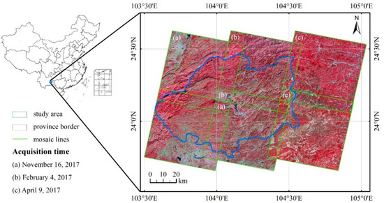
Figure 2.
Location of the study area and ZY-3 images of the study area. Qiubei county is located in the Yunnan Province of China.
2.2. ZY-3 Images and Pre-Processing
The ZY-3 is the first civil high-resolution stereoscopic Earth mapping satellite of China, launched on 9 January 2012 and designed to survey and monitor land resources. It is equipped with a multispectral sensor with 6 m spatial resolution and three high-resolution panchromatic cameras viewing looking in the forward, nadir, and backward direction. The spatial resolution of the three-line camera sensor is 3.5, 2.1, and 3.5 m, respectively. The multispectral sensor consists of four bands, including blue (450–520 nm), green (520–590 nm), red (630–690 nm), and near-infrared bands (770–890 nm). In our study, six ZY-3 multispectral images with different acquisition dates were acquired in 2017 (Figure 2). The seasonal variations of spectral signatures are limited due to the effects of tropical climate and the PN plantations are covered by black shade nets for a long time. Thus, PN plantations could be identified by analyzing the spectral signatures of black shade nets. The selection criteria for the images are not covered by the cloud (Figure 2). Six ZY-3 multispectral images were pre-processed in the Environment for Visualizing Images software (ENVI 5.3). Firstly, each ZY-3 image was processed using the orthorectification of the Rational Polynomial Coefficients (RPC) orthorectification module. Then, six ZY-3 images were corrected using the FLAASH Atmospheric Correction module. Thirdly, these images were mosaicked into one image using the Seamless Mosaic module. Finally, we obtained the resultant image of Qiubei county by clipping the mosaic image.
2.3. Methods
This methodological framework for PN mapping mainly consists of five consecutive phases (Figure 3): (1) the construction of new spectral index (NDPI); (2) conducting scale segmentation by using the BSM and selecting the optimal scale; (3) optimizing feature variables by iteration analysis; (4) using the RF classifier to implement the PN identification via the pixel-based, object-based, and IPOB methods, respectively; (5) accuracy assessment and spatial analyses on the three resultant maps.

Figure 3.
The methodological framework of PN mapping.
2.3.1. A New Spectral Index-Normalized Difference Panax Notoginseng Index (NDPI)-for Extracting Panax Notoginseng (PN)
We selected 3500 training samples based on a proportional random sampling method and conducted spectral signature analyses of buildings, vegetation, water, shadow, and PN. The random points of five types were generated according to the area percentage of each type derived from the government statistics bulletin. It is easy to choose train samples of buildings, vegetation, water, and shadow, while for the PN train samples, we choose the spectral signature of black shade nets as the spectral signature of PN in this study, because the black shade nets are accompanied by PN from planting to harvesting. Figure 4 shows that buildings have obvious different values in every band from that of PN; therefore, buildings can be separated from PN easily. Although PN has similar values with other vegetation in bands 1–3, their slopes between the green and near-infrared (NIR) bands show big differences. Thus, other vegetation can be separated from PN easily via NDVI. However, the water body and shadows cannot be separated easily from PN. Water and PN have strong absorption of incident energy (sunlight), showing a weak reflectivity and tending to further weaken as the wavelength increases. The reflectivity of PN in the Blue band is relatively strong, followed by the Green and Red bands, while the reflectivity of water in the Green band is the strongest. Given the role of the ratio method in distinguishing land types with large spectral differences, a Normalized Difference Panax notoginseng index (NDPI) was proposed in this study to discriminate better the PN and water body (Figure S1).
where is the value of the blue band, and is the value of the green band of the ZY-3 image.
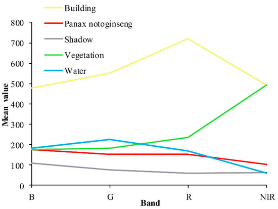
Figure 4.
Spectral signature analysis of five typical land cover samples in the study area.
2.3.2. Segmentation Optimization by Using the Bi-Level Scale-Sets Model (BSM)
Image segmentation represents a necessary and first prerequisite for object-based image analysis because the segmented objects form the basic unit of object-based image classification [36]. A group of pixels with similar spectral and spatial attributes is regarded as an object in the segmentation process [37]. In this study, image segmentation was performed using the bi-level scale-sets model (BSM) embedded in the SuperSIAT software, which is a powerful platform to provide the image segmentation and automatic scale optimization [38]. The fundamental of BSM is the scale-sets theory, which firstly represents an image using a region-based image hierarchy and secondly solves the scale problem in a high-level interpretation task [39]. Specifically, an image is divided into blocks with overlapped margins, and a low-level scale-sets model is achieved in the BSM. Then, the segmentation results of the whole image are obtained by mosaicking and retrieving the corresponding blocks and implementing a high-level scale-sets model.
In the low-level scale-sets model, six parameters need to be considered. First, the parameters K and Smin for the graph-based segmentation are regarded as the most crucial parameters because they directly bear the accuracy of the BSM. K refers to a constant parameter to control the size of the merged area, and Smin is the threshold for determining whether some small areas should be excluded. In general, larger K and Smin will result in fewer segments in a block, whereas smaller K and Smin will produce more segments in a block. Moreover, in the process of implementing the image hierarchy, the control of hierarchy quality depends on the merging cost criterion, which determines the order of merging. This merging cost criterion, including two parameters of wcolor and wshape, can be used to adjust spectrum and shape heterogeneity (Equation (2)) [40]. Within the wshape setting, the smoothness and compactness factors determining the object shape between smooth boundaries and compact edges can also be weighted, ranging from 0 to 1. In addition, there are two parameters in the BSM, including the average size of regions (Savr) in the link section and the width of a block (Wb). They are used to control the mosaicking of segmentation results from the low-level to high-level scale-sets model. A larger Savr implies fewer regions in the link section, and thus, the computation time of the high-level scale-sets model is reduced. According to previous studies [38], we set the values of the aforementioned parameters by using a large number of sample tests. The values of K, Smin, Wb, and Savr were 10, 5, 1000, and 200, respectively, which can guarantee classification accuracy and computational efficiency. Considering the PN has a striking color and regular shape in the image, the wcolor = 0.7 and wcompt = 0.5 were selected.
where and are the weight parameters, and . and are the color and shape differences of the two image objects to be merged.
The segmentation results acquired by the first step were used for the initial partition of the high-level scale-sets model. In this process, a scale parameter was required to implement the high-level scale-sets model of BSM. Three scale estimation methods embedded in the SuperSIAT software, including the Estimation of Scale Parameter (ESP) Method, Overall Goodness F-measure (OGF), and Bayesian method, could be used to rapidly and automatically select an optimal scale for the image classification [41]. The Bayesian method with an adjustable penalty factor (C) was used to estimate the optimal scale for the PN classification in this study, as it can indicate the optimal scale and avoid ambiguous results compared to the ESP method. The segmentation results ranged from over-segmentation to under-segmentation with the change of the C.
2.3.3. Feature Selection through Iterative Analysis
Compared to the pixel-based method, the object-based method may consider more features and not necessarily be constrained to spectral features. In this study, a total of 99 features categorized in four types (spectral, textural, geometric, and topographic types) were extracted from ZY-3 images (Supplementary Materials Table S1).
The textural features used to quantify the surface texture of image objects in this study were calculated by two approaches. The first approach is the Gray-Level Co-occurrence Matrix (GLCM), and its value indicates the frequency of occurrence in a particular spatial relationship between a pixel with intensity value i and a pixel with value j [7]. The second approach to measure textures is to use a Gray-Level Difference Vector (GLDV) and the sum of the diagonals of the GLCM. We evaluated considerable textural features including the GLCM (Homogeneity (Hom.), Contrast (Con.), Dissimilarity (Dis.), Entropy (Ent.), Angular 2nd moment (Ang.), Mean, StdDv., and Correlation (Cor.)) and GLDV (Contrast (Con.), Entropy (Ent.), Angular 2nd moment (Ang.), and Mean) for each band in all directions, as it could provide supplementary information about object attributes that can help discriminate heterogeneous regions [42].
The last is topographic features, which are very important attributes in image classification. The altitude and slope were considered in this study because the planting of PN is sensitive to topography, which was acquired from the DEM data derived from the ASTER Global Digital Elevation Map (GDEM) version 2 dataset with 30 m resolution. The four types of features for each object were used as input data in the RF classifier.
2.3.4. Random Forest Classifier with Optimized Parameters
The RF classifier is an ensemble classifier combining multiple decision trees proposed by Breiman [28] for regression and classification. Each tree is generated using a randomly selected subset of training samples and a random subset of independent variables, and then it votes for class membership. Finally, the classification result is obtained by assigning the respective class according to the maximum votes [43]. In the RF classifier, two parameters need to be considered, including the number of decision trees to be selected (Ntree) and the number of variables to be searched for the best splitting at each node (Mtry) [44]. The different Ntree and Mtry parameters could impact the classification accuracy, which is sensitive to the Mtry parameter proved in previous empirical research [45]. The value of Ntree can be set as large as possible because the RF classifier has high computational efficiency and is hard to overfit [46]. Some studies have also suggested that 500 is an acceptable value for the number of Ntree for the classifier [27]. The Mtry parameter is typically set to the square root of the total number of variables [13]. However, the default values of Ntree and Mtry parameters may not be suitable for all classification, so an optimizing parameter is needed for special classification. In this study, the out-of-bag samples (OOB) referred to samples without participating in training trees, which is about one-third of the total samples, and their errors were used to assess and select the optimal parameters.
Optimizing features is vital for improving classification accuracy, as the high-dimensional feature data in the classification process would lead to lower efficiency and model over-fitting [20]. The RF classifier has popular feature space optimization techniques with satisfactory results in multitudinous research fields [47,48]. Díaz-Uriarte and Andrés [49] proposed an iterative backward feature elimination procedure to reduce the number of less relevant variables and select the optimal features by the minimum OOB error. This procedure has been successfully used for feature selection in previous studies [50], and a similar iterative forward feature increase procedure was performed in this study. First, the variable importance (VI) was calculated and sorted from high to low by the RF classifier. Second, the most important variable was used as the input feature to acquire the OOB score. Then, we added one variable with subsequent important order as one of the input features in each loop iteration and estimated corresponding OOB scores. Finally, the optimal features were selected until the highest OOB score was reached.
2.3.5. Integrated Pixel- and Object-Based (IPOB) Approach for Mapping PN
In this study, a novel integrated pixel- and object-based (IPOB) approach was proposed to optimize PN mapping. The pixel-based classification may result in the mixed pixel problem and the “salt-and-pepper” effect [51,52,53]; these problems can be eliminated using object-based classification. However, new problems would emerge when using the object-based approach, e.g., the increased omission error from under-segmentation objects. Hence, the proposed IPOB approach aims to not only eliminate the “salt-and-pepper” effect from the pixel-based method but also decrease the omission error from the object-based method.
The framework of the IPOB approach involves two major stages (Figure 5). The first stage overlaps the two classification results from the pixel-based and object-based methods to generate the new segmentation unit of the IPOB approach. The overlapped criterion is shown in Figure 5: (1) If a PN object in the object-based classification result overlaps with a PN patch in the pixel-based classification result, they will be merged; (2) If the relationship between a PN object in the object-based classification result and a PN patch in the pixel-based classification result belongs to inclusion relations, the bigger one will be retained; (3) Independent PN patches in the pixel-based classification result will be retained; (4) Independent PN objects in the object-based classification result will be retained. The second stage is to classify PN using the optimal Random Forest classifier according to the segmentation units of the IPOB approach.

Figure 5.
The framework of the proposed IPOB approach in this study.
In terms of algorithm calibration, we also generated three sets of training samples to train the pixel-based RF classifier, object-based RF classifier, and IPOB RF classifier, respectively (Figure 6). To ensure that the classification results are not affected by the training samples, we implemented the following strategy to maximize the identity levels among different training sets as much as possible. First, we selected the training samples for the object-based RF classifier according to segmentation results. Then, the training samples for the pixel-based RF classifier were obtained by randomly generating several ROIs within each training sample of an object-based RF classifier. Finally, the training samples of the IPOB RF classifier were composed of the object-based training samples, a few mistaken pixels from the pixel-based classification result, and some missed pixels from the object-based classification result.
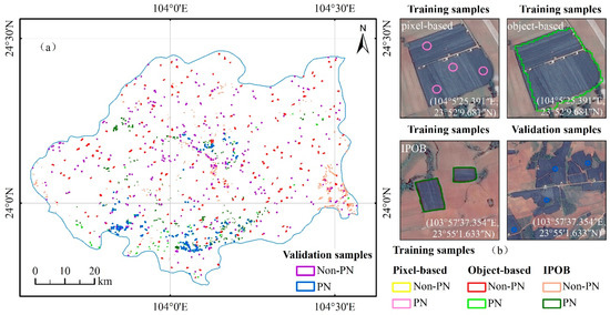
Figure 6.
Collection of training and validation samples for the Panax notoginseng mapping. (a) Spatial distribution of three sets of training and one set of validation samples; (b) four cases with different sample types from Google Earth images in 2017.
2.4. Validation of the Maps from the IPOB, Pixel-Based, and Object-Based Approaches and Their Intercomparison
Accuracy assessment is critical for land cover classification, especially the reliable reference data and suitable sampling method [54,55]. In this study, a random sampling method was used to obtain training and validation samples from the very high-resolution (VHR) images of Google Earth circa 2017. The validation samples were digitized through visual interpretation and double-checked by different researchers. We finally acquired a set of validation samples (in total 7056 pixels of PN and non-PN) to evaluate the accuracy of PN mapping from these three methods (Figure 6a).
In this study, we adopted the confusion matrix method to estimate the classification accuracies of different results by using the same validation samples. Producer accuracy (PA), user accuracy (UA), and F1-score (F1, Equation (3)) of PN from the confusion matrix was used to quantify the performance of the three approaches. We also compared the IPOB-based map and the pixel-based (or object-based) resultant map from both area and spatial distribution.
3. Results
3.1. Segmentation Optimization
The optimal segmentation units were obtained in the IPOB framework (Figure 7a). A large proportion of segmentation units were completely PN patches (Figure 7b). Some of the segmentation units were not PN patches (Figure 7c) because these segmentation units derived from the pixel-based classification result were misclassified due to their similar spectral features with PNs.
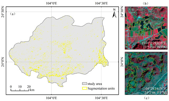
Figure 7.
The segmentation units mapped through the IPOB approach. (a) The optimal segmentation units from the IPOB framework; (b) zoom-in segmentation units of object-based classification result; (c) zoom-in segmentation units of the pixel-based classification result.
Three segmentation results at different scale parameters by using the object-based approach are shown in Figure 8. The image object for PN was over-segmented in Figure 8a, when the C was 10 and the segmentation scale was 50; while the image object for PN was under-segmented (Figure 8c) when the C was 0.71 and the corresponding segmentation scale was 150. The optimal segmentation scale of PN was obtained from the scale-sets model (Figure 8b) by adjusting the value of C. Here, the C was 3.59, and the corresponding optimal segmentation scale was 67.66.
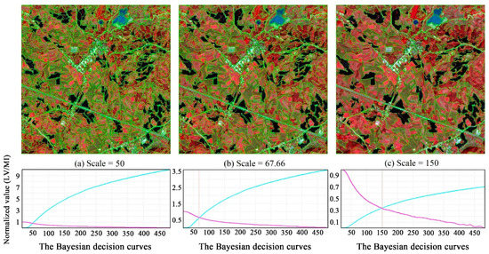
Figure 8.
Three segmentation results at different scale parameters and the corresponding values of the C parameter (the black parts are PN. LV: local variance, MI: Moran’s I). (a) the over-segmentation result (scale = 50, C = 10); (b) the optimal result (scale = 67.66, C = 3.59); (c) the under-segmentation result (scale = 150, C = 0.71).
3.2. Feature Selection
Figure 9 showed the importance of different features for identifying PN in the IPOB approach. The most important feature is DEM from topographic type because it can effectively discriminate against the PN and mountain shadow. Two subsequently important features are textural features, including GLCM_Hom of NIR band and GLCM_Mean. Compared with the order of importance for different features of pixel-based or object-based methods, the order of importance for different features in the IPOB approach has a larger difference because the segmentation units mainly involved PN patches and other patches with similar spectral features to PN.
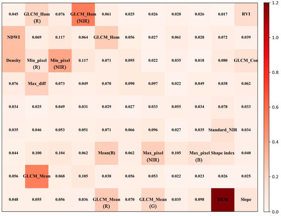
Figure 9.
The order of importance for different features (the most important 20 features were represented by names, others were represented by values. Spectral (10): Min_pixel (NIR), NDWI, Density, Mean (B), Max_diff, Min_pixel (R), Standard_NIR, Max_pixel (B), RVI, and Max_pixel (NIR); Textural (7): GLCM_Hom (NIR), GLCM_Mean, GLCM_Hom (R), GLCM_Hom, GLCM_Con, GLCM_Mean (R), and GLCM_Mean (G); Geometric (1): Shape index; Topographic (2): DEM, and Slope).
The relationship between the OOB Score and the number of features for IPOB PN mapping was shown in Figure 10a. This score increased rapidly in the first iteration and then became stable when exceeding 20 features, which showed a considerable number of features were redundant variables, leading to the high computational costs and over-fitting. The RF classifier with 55 features was identified as important variables for PN classification by analyses of the highest OOB score, including 20 spectral features, 25 textural features, 8 geometric features, and 2 geographical features.
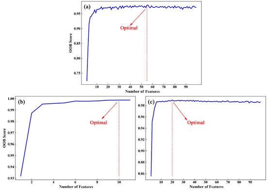
Figure 10.
Evolution of the out-of-bag samples (OOB) score related to the number of features: (a) the IPOB approach, (b) pixel-based approach, and (c) object-based approach.
When considering the pixel-based approach, nine spectral features and two geographical features were used to order the feature importance and select the optimal number of features (Figure 11). The first five features were spectral indexes, including NDWI, NDPI, NDVI, RVI, and DVI, where the most critical spectral index was NDWI, which was followed by the pixel value of four bands (NIR, R, G, and B). The last two features were geographical ones, including DEM and Slope. After variable selection, the 11th feature (Slope) was removed, and the rest of the features were used for PN mapping using a pixel-based approach (Figure 10b).
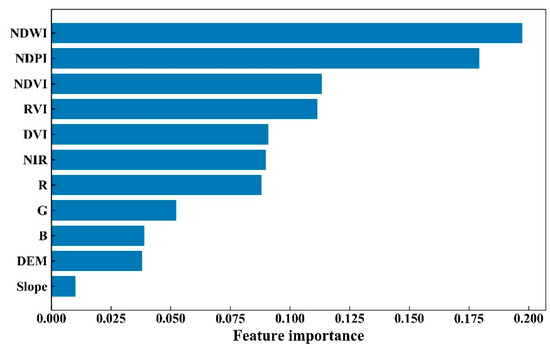
Figure 11.
The order of importance for different features in the pixel-based approach (Spectral (9): NDWI, NDPI, NDVI, RVI, DVI, NIR, R, G, B; Topographic (2): DEM, and Slope).
When only considering the object-based approach, features derived from the spectral type were dominant (Figure 12). The first four features included the new spectral index (NDPI), Mean of NIR band (Mean_NIR), NDWI, and the Min of NIR band (Min_NIR). Especially, the NDPI proposed in this study was the most important feature for PN identification. Furthermore, the geographic features, particularly DEM, were also very crucial in the classification process. The following important type was textural features, which could increase the classification accuracy by capturing the artificial texture of PN fields. A total of 20 features were selected to conduct PN mapping using the object-based approach (Figure 10c), including 13 spectral features, 6 textural features, and 1 geographical feature.
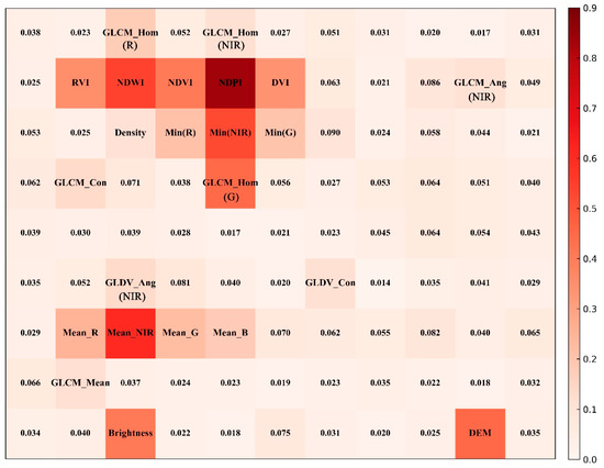
Figure 12.
The order of importance for different features (the most important 20 features were represented by name; others were represented by values. Spectral (13): NDPI, Mean_NIR, NDWI, Min_NIR, RVI, NDVI, DVI, Brightness, Min (R), Min (G), Mean_R, Mean_G, and Mean_B; Textural (6): GLCM_Hom (G), GLCM_Hom (NIR), GLCM_Hom (R), GLCM_Ang (NIR), GLCM_Con, and GLCM_Mean; Topographic (1): DEM).
3.3. Optimized Parameters of Random Forest Classifier
The optimized parameters (Mtry and Ntree) of the Random Forest classifier were calculated based on the minimum OOB errors. As shown in Figure 13a, the OOB errors of the IPOB approach in the RF classifier with different combinations of Mtry and Ntree range from approximately 0 to 0.35. Initially, the OOB errors decreased with a large Ntree, yet they tended to stabilize beyond 100 trees. Compared with Mtry = log2 or Mtry = None, Mtry = sqrt had a smaller value at a fixed value of Ntree and indicated that the optimal value of Mtry was sqrt. Therefore, the smallest OOB error appears at Mtry = sqrt and Ntree = 178. This combination of Mtry and Ntree was used to conduct the PN classification using the IPOB approach in the study area. When only considering the pixel-based approach, the optimal of Mtry and Ntree appeared at sqrt and 100 (Figure 13b). Similarly, the optimal of Mtry and Ntree for object-based approach appeared at sqrt and 378 (Figure 13c).
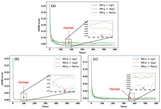
Figure 13.
The out-of-bag (OOB) errors between (a) IPOB, (b) pixel-based, and (c) object-based Random Forest classifier with different combinations of Mtry and Ntree.
3.4. Accuracy Assessment of Panax Notoginseng Mapping among IPOB, Pixel-Based and Object-Based Approaches
The classification accuracy of PN mapping based on the confusion matrix method is shown in Table 1. Compared with the pixel-based method, the object-based method has a higher F1-score (0.94 vs. 0.93). However, these two methods represented different advantages in user accuracy (UA) and producer accuracy (PA). To be specific, the object-based method has a higher UA (98.62% vs. 87.53%), while the pixel-based method has a higher PA (99.15% vs. 90%), which indicates that the object-based method tends to omit PN objects while the pixel-based method may misclassify PN pixels. Based on these two features, the IPOB approach was proposed to combine the advantages of object-based and pixel-based methods. In terms of three PN mapping approaches, the highest F1-score (0.98) in the IPOB approach indicates its ability to identify PN accurately. Meanwhile, the UA of the IPOB approach outperformed the object-based method (97.36% vs. 98.62%) and higher by 9.83% compared to that of the pixel-based method. The PA of the IPOB approach has exceeded that of the pixel-based method (99.22% vs. 99.15%) and was higher by 9.22% compared to that of the object-based method.

Table 1.
Accuracy assessment of Panax notoginseng mapping by using confusion matrix.
3.5. Spatial and Area Comparisons among the Three PN Maps
Generally, three PN maps showed relatively good consistency (Figure 14). In this region, about 0.44% and 98.86% of pixels in the study area were identified as consistent PN and non-PN by those three PN maps. In detail, the total consistent PN area of the IPOB and pixel-based approaches was estimated to be 29.59 km², which was higher than that of the IPOB and object-based approaches (26.54 km²) (Figure 15). Moreover, the total PN area was estimated at 36.36 km² according to the IPOB-based approach, while 50.45 km² and 26.55 km² of which were evaluated according to the pixel-based approach and the object-based approach, respectively. Compared with the IPOB-based approach, the total PN area from the pixel-based approach was overestimated, and these inconsistent PN pixels (about 20.85 km²) were mainly distributed in the eastern of Qiubei county (Figure 15a). In addition, the total PN area from the object-based approach was underestimated by 6.76 km² (Figure 15b).
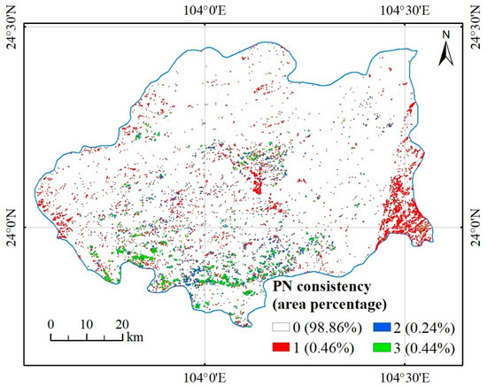
Figure 14.
Spatial distribution map of the Panax notoginseng frequency from IPOB map, pixel-based map, and object-based map.

Figure 15.
Spatial comparison between the IPOB map, (a) pixel-based map, and (b) object-based map.
4. Discussion
4.1. Innovativeness of the Panax Notoginseng Mapping
In this study, a new framework of PN mapping by integrating pixel-based and object-based approaches (IPOB) was built, which performed the predominant performance and potential for identifying PN. This study also improved PN mapping in different ways, including proposing a new spectral index-Normalized Difference PN Index (NDPI), optimizing the efficiency and scale of segmentation using the bilevel scale-sets model (BSM) and feature selection through an iteration analysis. Specifically, compared with some of the previous studies for plantation mapping, this study improved the existing efforts in several aspects:
First, the resolution of source data has been improved in comparison to previous studies. Shi, Zhang, Guo, and Huang [9] adopted the GF-1 multispectral remote sensing data with 16 m resolution and Dai, Xie, Zhigang, and Peijun [5] used the Landsat image with 30 m resolution, while we applied the ZY-3 images with 6 m resolution, which is approximately 1/3 of the former and 1/5 of the latter. Figure 16 explicated that the higher resolution imagery can greatly reduce the potential omission errors in PN mapping. The PN in the green and blue regions could be distinctly identified by the object-based method with the ZY-3 images (Figure 16a). For the GF-1 WFV images, the PN in the green region may be identified, but the blue region was difficult to be identified (Figure 16b). However, it was hard to identify PNs within the green and blue regions of the Landsat images (Figure 16c), especially when the area of the blue region, which was smaller than one pixel. An enormous number of PN areas had field sizes of less than 1 km² in this study area. Therefore, high-resolution images were necessary for PN identification. A similar conclusion had been found in previous studies (Duro et al., 2012; Myint et al., 2011; Robertson and King 2011). They found that the object-based method was more suitable for the classification of high-resolution data rather than that of coarse resolution data, and they had a noticeable predominance for representing some of the land cover types with the generalized appearance, such as croplands.
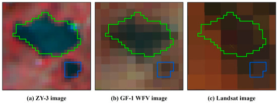
Figure 16.
Two PN fields are shown in three different images: (a) ZY-3 image with 6 m resolution, (b) GF-1 WFV image with 16 m resolution, (c) Landsat image with 30 m resolution (green: area > 1 km², blue: area < 1 km²).
Second, a novel spectral index (NDPI) was proposed as an important variable in the classification. To further clarify the contribution of NDPI, we conducted the workflow again under the same condition but removing the NDPI. Table 2 showed the classification accuracy of the PN map without NDPI from the pixel-based, object-based, and IPOB approaches, respectively. Specifically, the IPOB approach has a high F1-score (0.94). The object-based PN map and pixel-based PN map showed the low F1-score (0.92) due to the larger omit error from the object-based approach (PA = 86.49%) and commission error from the pixel-based approach (UA = 86.2%). However, the accuracies of the PN maps without NDPI from these three methods were lower than that of the PN map with NDPI, which indicated that the NDPI has a significant influence on omission error. Hence, the contribution of NDPI may help to enhance the feature difference between PN and Non-PN when using the object-based method and decrease potential omission errors in the classification process.
Table 2.
Accuracy assessment of the Panax notoginseng map without involving NDPI.
Third, a new IPOB approach was proposed by integrating the pixel-based and object-based methods. Previous studies have found some shortages using solely the pixel-based or object-based classification method [56]. The pixel-based method may lead to the “salt-and-pepper” effect, while the object-based method has been found with some problems with lower processing efficiency and inconsistent segmentation scale with the real-world objects (Blaschke 2001). The integration of the pixel-based and object-based methods has been proved that it can eliminate the “salt-and-pepper” effect and improve classification efficiency. Figure 17 illustrated the disadvantages of the pixel-based and object-based methods and the advantage of the IPOB approach. On the one hand, Figure 17a,b showed that the PN object at the location of B2 was not identified due to the large segmentation unit of A2. Figure 17c showed that PN pixels were identified well, but there was the “salt-and-pepper” effect at the location of C1. On the other hand, the IPOB approach generated new segmentation units (Figure 17e) and obtained more accurate classification results via the RF classifier. Figure 17f showed that the IPOB PN mapping result eliminated the “salt-and-pepper” effect in the pixel-based method and picked up potentially omitted PN objects in the object-based method.
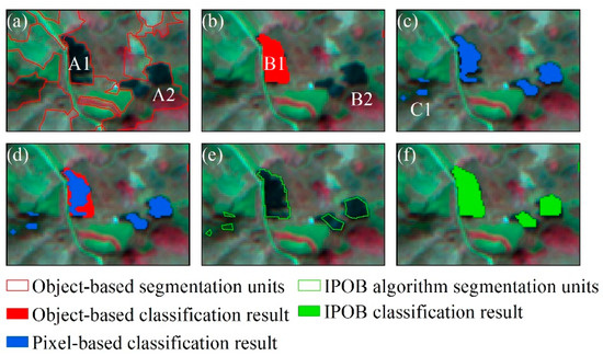
Figure 17.
The calculate framework of the IPOB approach; (a) the segmentation scale of object-based, (b) object-based classification result, (c) pixel-based classification result, (d) overlapped result of pixel-based and object-based classification results, (e) IPOB approach segmentation units, (f) IPOB classification result.
Finally, using the BSM and optimal parameters in this IPOB framework effectively improved the classification accuracy and reduced the computation time. A large number of studies have indicated that the optimal segmentation scale was considerably important to improve classification accuracy [19]. However, in previous studies, the segmentation scales were selected through a trial-and-error method [57,58], which is subjective, time-consuming, and prone to produce errors [13]. For example, Peña-Barragán, Ngugi, Plant, and Six [7] selected the optimal segmentation parameters using 1312 different segmentation scenarios, which was an enormous project. In this study, the Bayesian method in the SuperSIAT software was used to rapidly estimate an optimal scale parameter from a recorded scale-indexed tree structure, avoiding repeated segmentation procedure in eCognition software. Optimizing the Mtry and Ntree parameters was a vital factor for improving classification accuracy [59], which was conducted in RF classifier in this study. In terms of computation time, BSM takes less than 6 min to obtain image segmentation results with 20,000 × 20,000 pixels on a common computer (CPU: Intel Xeon(R) 2.90GHz, RAM: 32GB, OS: Windows10). The segmentation efficiency is about two to three times faster than eCognition software 9.2.
4.2. Implications of the Panax Notoginseng Mapping
In this study, we proposed a novel IPOB approach by integrating pixel-based and object-based methods to generate PN mapping. This method showed a predominant advantage for PN mapping, as it could help to decrease errors and improve classification efficiency. Traditional pixel-based methods can rapidly conduct classification, but the mapping accuracy is unable to meet a realistic requirement. Compared to the pixel-based method, the object-based method had an overwhelming superiority in integrating spectral, textural, and geometric features, improving classification accuracy, and representing real-world correspondence [60]. However, it has not been widely applied mainly because of its complexity in parameter selection and computation efficiency for large-scale mapping [61]. Myint et al. [62] indicated that it was difficult to perform many features or bands for multiscale segmentation and classification in eCognition software due to computer memory limitation. Hence, balancing the time cost and classification accuracy was a significant factor in selecting classification methods [17]. Quantitating optimal segmentation models and parameters (e.g., BSM) to reduce computation time as well as selecting suitable features from hundreds of object features need more effort in future studies [32]. This study indicates that combining the IPOB approach and BSM can improve classification accuracy and efficiency, suggesting the potential for large-scale mapping.
To better formulate the identification framework, the relationship between certain land covers and their surroundings needs to be considered. Land covers that are very different from the surrounding environment such as water and vegetation are easy to identify. However, it is challenging to identify PN in a true color composite image, as the image feature of PN is similar to water and shadow. Hence, in our study, we first considered the planting situation of PN (including its suitable altitude and slope) to help us identify PN and shadow. Then, we analyzed spectral feature differences between PN and water, showing the largest difference in the green band and the smallest difference in the blue band. Based on this foundation, NDPI was proposed in this study to better discriminate the PN and water areas. Finally, the images are classified by considering the spectral and topographic types and showed the highest classification accuracy. In future vegetation mapping, we should comprehensively consider the growth habits, spectral, textural, geometric, and phenological characteristics of vegetation types, and combine the differences in image spectral characteristics to identify vegetation types in complex environments. For other types of images, the new index will work well by using similar sensors such as Sentinel-2A/B, which could provide improved spatial resolution (10 m). This work may also provide some reference for mapping other types of herbs (e.g., Ginseng, Coptidis) in different regions; however, specific characteristics of different herbs should be considered before its application.
The medical value of PN has been demonstrated and widely studied [63,64], while the distribution of PN was rarely concerned by researchers. Monitoring the distribution and planting of PN is very important to regulate the market price of the government and serve the medical treatment of humans. Given strict growth conditions, the suitable planting regions of PN are very limited in China. A few studies analyzed the suitable planting region of PN in the world [65], which showed that the most suitable planting region of PN was China and the potential planting regions include the United States, Brazil, Portugal, and other 22 countries. It also suggested that the distribution of PN should be investigated using a remote sensing method to provide a precise base for the selection of PN samples in the future. Precisely, the resultant maps from our study can provide valuable information for analyzing the suitable planting region of PN in the world.
5. Conclusions
There is limited knowledge on the area and distribution of traditional Chinese medicine resources such as Panax notoginseng (PN), which leads to difficulties in regional land use management and planning. Here, we developed a novel methodological framework for PN mapping by integrating the pixel-based and object-based (IPOB) methods. The result showed a higher F1-score of 0.98 compared with the solely pixel-based or object-based method, suggesting the high robustness of the IPOB framework. Some improvements have been conducted within the framework. First, a parallel segmentation approach from the bilevel scale-sets model (BSM) significantly improved segmentation efficiency in this study. Second, all parameters and feature variables were optimized in the RF classifier to improve the classification accuracy. Third, a novel spectral index (NDPI) was proposed and played an essential role in reducing the number of optimal features and improving classification accuracy. This study provided a demo for mapping traditional Chinese medicine resources based on remote sensing technology, and the approach can be used for investigating other medicine plantations.
Supplementary Materials
The following are available online at https://www.mdpi.com/article/10.3390/rs13112184/s1, Figure S1: Scatter plot regarding the NDPI of the PN and water, Table S1: Overview of computed features for each object.
Author Contributions
Conceptualization, Z.Y. and J.D.; methodology, Z.Y.; investigation and data curation, Z.Y. and W.K.; writing—original draft preparation, Z.Y.; writing—review and editing, J.D., Y.Q., and X.X.; supervision, J.D. and X.X.; project administration, J.D.; funding acquisition, J.D. All authors have read and agreed to the published version of the manuscript.
Funding
This study is funded by the Key Research Program of Frontier Sciences (QYZDB-SSW-DQC005) and the Strategic Priority Research Program (XDA19040301) of the Chinese Academy of Sciences (CAS).
Institutional Review Board Statement
Not applicable.
Informed Consent Statement
Not applicable.
Data Availability Statement
The data presented in this study are available on request from the corresponding author.
Acknowledgments
We thank Dengsheng Lu, Guosong Zhao, Yupeng Fan, Nanshan You, and Arifuzzaman Khondakar for their comments on the initial draft. We are also indebted to the five anonymous reviewers for their fruitful suggestions.
Conflicts of Interest
The authors declare no conflict of interest.
References
- Yang, C.W.; Zhu, Y.Y.; Zhang, R.K.; Ning, W.Y. Studies on the Engineering and Technical System of Integrating Agricultural Machinery and Agronomic Based on Sustainable Development of Panax Notoginseng Industry. Hubei Agric. Sci. 2014, 53, 122–125. [Google Scholar]
- Cui, X.M.; Huang, L.Q.; Guo, L.P.; Liu, D.H. Chinese Sanqi Industry Status and Development Countermeasures. China J. Chin. Mater. Med. 2014, 39, 553. [Google Scholar]
- Zhao, G.R.; Xiang, Z.J.; Ye, T.X.; Yuan, Y.J.; Guo, Z.X. Antioxidant Activities of Salvia Miltiorrhiza and Panax Notoginseng. Food Chem. 2006, 99, 767–774. [Google Scholar] [CrossRef]
- Zhang, Z.-L.; Wang, W.-Q.; Miu, Z.-Q.; Li, S.-D.; Yang, J.-Z. Application of Principal Component Analysis in Comprehensive Assessment of Soil Quality under Panax Notoginseng Continuous Planting. Chin. J. Ecol. 2013, 321, 636–644. [Google Scholar]
- Dai, C.; Xie, X.; Xu, Z.; Du, P. Monitoring and Analyzing Herbal Medicine Plantation Via Remote Sensing:A Case Study of Pseudo-Ginseng in Wenshan and Honghe Prefecture of Yunnan Province. Remote Sens. Land Resour. 2018, 30, 210–216. [Google Scholar]
- Long, H.; Liu, Y.; Hou, X.; Li, T.; Li, Y. Effects of Land Use Transitions Due to Rapid Urbanization on Ecosystem Services: Implications for Urban Planning in the New Developing Area of China. Habitat Int. 2014, 44, 536–544. [Google Scholar] [CrossRef]
- Peña-Barragán, J.M.; Ngugi, M.K.; Plant, R.E.; Six, J. Object-Based Crop Identification Using Multiple Vegetation Indices, Textural Features and Crop Phenology. Remote Sens. Environ. 2011, 115, 1301–1316. [Google Scholar] [CrossRef]
- Dong, J.; Xiao, X.; Menarguez, M.A.; Zhang, G.; Qin, Y.; Thau, D.; Biradar, C.; Iii, B.M. Mapping Paddy Rice Planting Area in Northeastern Asia with Landsat 8 Images, Phenology-Based Algorithm and Google Earth Engine. Remote Sens. Environ. 2016, 185, S003442571630044X. [Google Scholar] [CrossRef]
- Shi, T.T.; Zhang, X.B.; Guo, L.P.; Huang, L.Q. Study on Extraction Method of Panax Notoginseng Plots in Wenshan of Yunnan Province Based on Decision Tree Model. China J. Chin. Mater. Med. 2017, 42, 4358–4361. [Google Scholar]
- Blaschke, T. What’s Wrong with Pixels? Some Recent Developments Interfacing Remote Sensing and Gis. GeoBIT/GIS 2001, 6, 12–17. [Google Scholar]
- Hussain, M.; Chen, D.; Cheng, A.; Wei, H.; Stanley, D. Change Detection from Remotely Sensed Images: From Pixel-Based to Object-Based Approaches. ISPRS J. Photogramm. Remote Sens. 2013, 80, 91–106. [Google Scholar] [CrossRef]
- Johansen, K.; Arroyo, L.A.; Phinn, S.; Witte, C.; Hay, G.J.; Blaschke, T. Comparison of Geo-Object Based and Pixel-Based Change Detection of Riparian Environments Using High Spatial Resolution Multi-Spectral Imagery. Photogramm. Eng. Remote Sens. 2010, 76, 123–136. [Google Scholar] [CrossRef]
- Puissant, A.; Rougier, S.; Stumpf, A. Object-Oriented Mapping of Urban Trees Using Random Forest Classifiers. Int. J. Appl. Earth Obs. Geoinf. 2014, 26, 235–245. [Google Scholar] [CrossRef]
- Blaschke, T. Object Based Image Analysis for Remote Sensing. ISPRS J. Photogramm. Remote Sens. 2010, 65, 2–16. [Google Scholar] [CrossRef]
- Blaschke, T.; Hay, G.J.; Kelly, M.; Lang, S.; Hofmann, P.; Addink, E.; Feitosa, R.Q.; van der Meer, F.; van der Werff, H.; van Coillie, F.; et al. Geographic Object-Based Image Analysis—Towards a New Paradigm. ISPRS J. Photogramm. Remote Sens. 2014, 87, 180–191. [Google Scholar] [CrossRef] [PubMed]
- Li, M.; Ma, L.; Blaschke, T.; Cheng, L.; Tiede, D. A Systematic Comparison of Different Object-Based Classification Techniques Using High Spatial Resolution Imagery in Agricultural Environments. Int. J. Appl. Earth Obs. Geoinf. 2016, 49, 87–98. [Google Scholar] [CrossRef]
- Duro, D.C.; Franklin, S.E.; Dubé, M.G. A Comparison of Pixel-Based and Object-Based Image Analysis with Selected Machine Learning Algorithms for the Classification of Agricultural Landscapes Using Spot-5 Hrg Imagery. Remote Sens. Environ. 2012, 118, 259–272. [Google Scholar] [CrossRef]
- Keyport, R.N.; Oommen, T.; Martha, T.R.; Sajinkumar, K.S.; Gierke, J.S. A Comparative Analysis of Pixel- and Object-Based Detection of Landslides from Very High-Resolution Images. Int. J. Appl. Earth Obs. Geoinf. 2018, 64, 1–11. [Google Scholar] [CrossRef]
- Ma, L.; Li, M.; Ma, X.; Cheng, L.; Du, P.; Liu, Y. A Review of Supervised Object-Based Land-Cover Image Classification. ISPRS J. Photogramm. Remote Sens. 2017, 130, 277–293. [Google Scholar] [CrossRef]
- Chen, T.; Trinder, J.C.; Niu, R. Object-Oriented Landslide Mapping Using Zy-3 Satellite Imagery, Random Forest and Mathematical Morphology, for the Three-Gorges Reservoir, China. Remote Sens. 2017, 9, 333. [Google Scholar] [CrossRef]
- Ma, L.; Cheng, L.; Li, M.; Liu, Y.; Ma, X. Training Set Size, Scale, and Features in Geographic Object-Based Image Analysis of Very High Resolution Unmanned Aerial Vehicle Imagery. ISPRS J. Photogramm. Remote Sens. 2015, 102, 14–27. [Google Scholar] [CrossRef]
- Möller, M.; Lymburner, L.; Volk, M. The Comparison Index: A Tool for Assessing the Accuracy of Image Segmentation. Int. J. Appl. Earth Obs. Geoinf. 2007, 9, 311–321. [Google Scholar] [CrossRef]
- Drǎguţ, L.; Tiede, D.; Levick, S.R. Esp: A Tool to Estimate Scale Parameter for Multiresolution Image Segmentation of Remotely Sensed Data. Int. J. Geogr. Inf. Sci. 2010, 24, 859–871. [Google Scholar] [CrossRef]
- Costa, H.; Carrão, H.; Bação, F.; Caetano, M. Combining Per-Pixel and Object-Based Classifications for Mapping Land Cover over Large Areas. Int. J. Remote Sens. 2014, 35, 738–753. [Google Scholar] [CrossRef]
- Yang, L.; Jin, S.; Danielson, P.; Homer, C.; Gass, L.; Bender, S.M.; Case, A.; Costello, C.; Dewitz, J.; Fry, J.; et al. A New Generation of the United States National Land Cover Database: Requirements, Research Priorities, Design, and Implementation Strategies. ISPRS J. Photogramm. Remote Sens. 2018, 146, 108–123. [Google Scholar] [CrossRef]
- Lu, D.; Weng, Q. A Survey of Image Classification Methods and Techniques for Improving Classification Performance. Int. J. Remote Sens. 2007, 28, 823–870. [Google Scholar] [CrossRef]
- Belgiu, M.; Drăguţ, L. Random Forest in Remote Sensing: A Review of Applications and Future Directions. ISPRS J. Photogramm. Remote Sens. 2016, 114, 24–31. [Google Scholar] [CrossRef]
- Breiman, L. Random Forests. Mach. Learn. 2001, 45, 5–32. [Google Scholar] [CrossRef]
- Rodriguez-Galiano, V.F.; Ghimire, B.; Rogan, J.; Chica-Olmo, M.; Rigol-Sanchez, J.P. An Assessment of the Effectiveness of a Random Forest Classifier for Land-Cover Classification. ISPRS J. Photogramm. Remote Sens. 2012, 67, 93–104. [Google Scholar] [CrossRef]
- Pelletier, C.; Valero, S.; Inglada, J.; Champion, N.; Dedieu, G. Assessing the Robustness of Random Forests to Map Land Cover with High Resolution Satellite Image Time Series over Large Areas. Remote Sens. Environ. 2016, 187, 156–168. [Google Scholar] [CrossRef]
- Han, H.; Lee, S.; Im, J.; Kim, M.; Lee, M.I.; Ahn, M.H.; Chung, S.R. Detection of Convective Initiation Using Meteorological Imager Onboard Communication, Ocean, and Meteorological Satellite Based on Machine Learning Approaches. Remote Sens. 2015, 7, 9184–9204. [Google Scholar] [CrossRef]
- Chan, J.C.-W.; Paelinckx, D. Evaluation of Random Forest and Adaboost Tree-Based Ensemble Classification and Spectral Band Selection for Ecotope Mapping Using Airborne Hyperspectral Imagery. Remote Sens. Environ. 2008, 112, 2999–3011. [Google Scholar] [CrossRef]
- Berhane, T.M.; Lane, C.R.; Wu, Q.; Autrey, B.C.; Anenkhonov, O.A.; Chepinoga, V.V.; Liu, H. Decision-Tree, Rule-Based, and Random Forest Classification of High-Resolution Multispectral Imagery for Wetland Mapping and Inventory. Remote Sens. 2018, 10, 580. [Google Scholar] [CrossRef] [PubMed]
- Abdel-Rahman, E.M.; Mutanga, O.; Adam, E.; Ismail, R. Detecting Sirex Noctilio Grey-Attacked and Lightning-Struck Pine Trees Using Airborne Hyperspectral Data, Random Forest and Support Vector Machines Classifiers. ISPRS J. Photogramm. Remote Sens. 2014, 88, 48–59. [Google Scholar] [CrossRef]
- Vetrivel, A.; Gerke, M.; Kerle, N.; Vosselman, G. Identification of Damage in Buildings Based on Gaps in 3d Point Clouds from Very High Resolution Oblique Airborne Images. ISPRS J. Photogramm. Remote Sens. 2015, 105, 61–78. [Google Scholar] [CrossRef]
- Castilla, G.; Hay, G.J. Object-Based Image Analysis; Springer: Berlin, Germany, 2008; pp. 91–110. [Google Scholar]
- Walter, V. Object-Based Classification of Remote Sensing Data for Change Detection. ISPRS J. Photogramm. Remote. 2004, 58, 225–238. [Google Scholar] [CrossRef]
- Hu, Z.; Li, Q.; Zou, Q.; Zhang, Q.; Wu, G. A Bilevel Scale-Sets Model for Hierarchical Representation of Large Remote Sensing Images. IEEE Trans. Geosci. Remote Sens. 2016, 54, 7366–7377. [Google Scholar] [CrossRef]
- Guigues, L.; Cocquerez, J.P.; Le Men, H. Scale-Sets Image Analysis. Int. J. Comput. Vis. 2006, 68, 289–317. [Google Scholar] [CrossRef]
- Baatz, M.; Schape, A. Angewandte Geographische Informationsverarbeitung; Wichmann: Heidelberg, Germany, 2000; pp. 12–23. [Google Scholar]
- Hu, Z.; Zhang, Q.; Zou, Q.; Li, Q.; Wu, G. Stepwise Evolution Analysis of the Region-Merging Segmentation for Scale Parameterization. IEEE J. Sel. Top. Appl. Earth Obs. Remote Sens. 2018, 11, 2461–2472. [Google Scholar] [CrossRef]
- Pacifici, F.; Chini, M.; Emery, W.J. A Neural Network Approach Using Multi-Scale Textural Metrics from Very High-Resolution Panchromatic Imagery for Urban Land-Use Classification. Remote Sens. Environ. 2009, 113, 1276–1292. [Google Scholar] [CrossRef]
- Stumpf, A.; Kerle, N. Object-Oriented Mapping of Landslides Using Random Forests. Remote Sens. Environ. 2011, 115, 2564–2577. [Google Scholar] [CrossRef]
- Rodriguez-Galiano, V.F.; Chica-Olmo, M.; Abarca-Hernandez, F.; Atkinson, P.M.; Jeganathan, C. Random Forest classification of Mediterranean land cover using multi-seasonal imagery and multi-seasonal texture. Remote Sens. Environ. 2012, 121, 93–107. [Google Scholar] [CrossRef]
- Ghosh, A.; Fassnacht, F.E.; Joshi, P.K.; Koch, B. A Framework for Mapping Tree Species Combining Hyperspectral and Lidar Data: Role of Selected Classifiers and Sensor across Three Spatial Scales. Int. J. Appl. Earth Obs. Geoinf. 2014, 26, 49–63. [Google Scholar] [CrossRef]
- Guan, H.; Li, J.; Chapman, M.; Deng, F.; Ji, Z.; Yang, X. Integration of Orthoimagery and Lidar Data for Object-Based Urban Thematic Mapping Using Random Forests. Int. J. Remote Sens. 2013, 34, 5166–5186. [Google Scholar] [CrossRef]
- Cavallaro, G.; Mura, M.D.; Benediktsson, J.A.; Bruzzone, L. Extended Self-Dual Attribute Profiles for the Classification of Hyperspectral Images. IEEE Geosci. Remote Sens. Lett. 2015, 12, 1690–1694. [Google Scholar] [CrossRef]
- Demarchi, L.; Canters, F.; Cariou, C.; Licciardi, G.; Chan, C.W. Assessing the Performance of Two Unsupervised Dimensionality Reduction Techniques on Hyperspectral Apex Data for High Resolution Urban Land-Cover Mapping. ISPRS J. Photogramm. Remote Sens. 2014, 87, 166–179. [Google Scholar] [CrossRef]
- Díaz-Uriarte, R.; de Andrés, S.A. Gene Selection and Classification of Microarray Data Using Random Forest. BMC Bioinform. 2006, 7, 3. [Google Scholar] [CrossRef]
- Gregorutti, B.; Michel, B.; Saint-Pierre, P. Correlation and Variable Importance in Random Forests. Stat. Comput. 2013, 27, 659–678. [Google Scholar] [CrossRef]
- Laliberte, A.S.; Rango, A.; Havstad, K.M.; Paris, J.F.; Beck, R.F.; Mcneely, R.; Gonzalez, A.L. Object-Oriented Image Analysis for Mapping Shrub Encroachment from 1937 to 2003 in Southern New Mexico. Remote Sens. Environ. 2004, 93, 198–210. [Google Scholar] [CrossRef]
- Chen, G.; Hay, G.J.; Carvalho, L.M.T.; Wulder, M.A. Object-Based Change Detection. Int. J. Remote Sens. 2012, 33, 4434–4457. [Google Scholar] [CrossRef]
- Aplin, P. On Scales and Dynamics in Observing the Environment. Int. J. Remote Sens. 2006, 27, 2123–2140. [Google Scholar] [CrossRef]
- Congalton, R.G. A Review of Assessing the Accuracy of Classifications of Remotely Sensed Data. Remote Sens. Environ. 1998, 37, 270–279. [Google Scholar] [CrossRef]
- Yang, Z.; Dong, J.; Qin, Y.; Ni, W.; Zhao, G.; Chen, W.; Chen, B.; Kou, W.; Wang, J.; Xiao, X. Integrated Analyses of Palsar and Landsat Imagery Reveal More Agroforests in a Typical Agricultural Production Region, North China Plain. Remote Sens. 2018, 10, 1323. [Google Scholar] [CrossRef]
- Xiong, J.; Thenkabail, P.; Tilton, J.; Gumma, M.; Teluguntla, P.; Oliphant, A.; Congalton, R.; Yadav, K.; Gorelick, N. Nominal 30-M Cropland Extent Map of Continental Africa by Integrating Pixel-Based and Object-Based Algorithms Using Sentinel-2 and Landsat-8 Data on Google Earth Engine. Remote Sens. 2017, 9, 1065. [Google Scholar] [CrossRef]
- Robertson, L.D.; King, D. Comparison of Pixel- and Object-Based Classification in Land Cover Change Mapping. Int. J. Remote Sens. 2011, 32, 1505–1529. [Google Scholar] [CrossRef]
- Ballanti, L.; Blesius, L.; Hines, E.; Kruse, B. Tree Species Classification Using Hyperspectral Imagery: A Comparison of Two Classifiers. Remote Sens. 2016, 8, 445. [Google Scholar] [CrossRef]
- Corcoran, J.M.; Knight, J.F.; Gallant, A.L. Influence of Multi-Source and Multi-Temporal Remotely Sensed and Ancillary Data on the Accuracy of Random Forest Classification of Wetlands in Northern Minnesota. Remote Sens. 2013, 5, 3212–3238. [Google Scholar] [CrossRef]
- Addink, E.A.; van Coillie, F.M.B.; de Jong, S.M. Introduction to the Geobia 2010 Special Issue: From Pixels to Geographic Objects in Remote Sensing Image Analysis. Int. J. Appl. Earth Obs. Geoinf. 2012, 15, 1–6. [Google Scholar] [CrossRef]
- Platt, R.V.; Rapoza, L. An Evaluation of an Object-Oriented Paradigm for Land Use/Land Cover Classification. Prof. Geogr. 2008, 60, 87–100. [Google Scholar] [CrossRef]
- Myint, S.W.; Gober, P.; Brazel, A.; Grossman-Clarke, S.; Weng, Q. Per-Pixel Vs. Object-Based Classification of Urban Land Cover Extraction Using High Spatial Resolution Imagery. Remote Sens. Environ. 2011, 115, 1145–1161. [Google Scholar] [CrossRef]
- Sun, S.; Wang, C.Z.; Tong, R.; Li, X.L.; Fishbein, A.; Wang, Q.; He, T.C.; Du, W.; Yuan, C.S. Effects of Steaming the Root of Panax Notoginseng on Chemical Composition and Anticancer Activities. Food Chem. 2016, 118, 307–314. [Google Scholar] [CrossRef]
- Yang, Z.G.; Sun, H.X.; Ye, Y.P. Ginsenoside Rd from Panax Notoginseng Is Cytotoxic Towards Hela Cancer Cells and Induces Apoptosis. Chem. Biodivers. 2010, 3, 187–197. [Google Scholar] [CrossRef] [PubMed]
- Meng, X.X.; Huang, L.F.; Dong, L.L.; Li, X.W.; Wei, F.G.; Chen, Z.J.; Wu, J.; Sun, C.Z.; Yu, Y.Q.; Chen, S.L. Analysis of Global Ecology of Panax Notoginseng in Suitability and Quality. Acta Pharm. Sin. 2016, 51, 1483–1493. [Google Scholar]


Publisher’s Note: MDPI stays neutral with regard to jurisdictional claims in published maps and institutional affiliations. |
© 2021 by the authors. Licensee MDPI, Basel, Switzerland. This article is an open access article distributed under the terms and conditions of the Creative Commons Attribution (CC BY) license (https://creativecommons.org/licenses/by/4.0/).