A New Approach for Cylindrical Steel Structure Deformation Monitoring by Dense Point Clouds

Abstract

As fundamental load-bearing parts, the cylindrical steel structures of transmission towers relate to the stability of the main structures in terms of topological relation and performance. Therefore, the periodic monitoring of a cylindrical steel structure is necessary to maintain the safety and stability of existing structures in energy transmission. Most studies on deformation analysis are still focused on the process of identifying discrepancies in the state of a structure by observing it at different times, yet relative deformation analysis based on the data acquired in single time has not been investigated effectively. In this study, the piecewise cylinder fitting method is presented to fit the point clouds collected at a single time to compute the relative inclination of a cylindrical steel structure. The standard deviation is adopted as a measure to evaluate the degree of structure deformation. Meanwhile, the inclination rate of each section is compared with the conventional method on the basis of the piecewise cylinder fitting parameters. The validity and accuracy of the algorithm are verified by real transmission tower point cloud data. Experimental results show that the piecewise cylinder fitting algorithm proposed in this research can meet the accuracy requirements of cylindrical steel structure deformation analysis and has high application value in the field of structure deformation monitoring.

1. Introduction

Electric power has become the main energy to support the normal operation of the infrastructure of a society, and maintaining its smooth and safe transmission is of significance. The structure of a cylindrical shape is one of the most common and extended structures present in the field of transformer substation, which serves as the basic component to support the main structures of energy transmission. Its structural safety directly relates to the stability of the main structures in terms of topological relation and performance. However, as fundamental load-bearing parts under long-time services, the cylindrical steel structures of transmission tower tend to be corroded and tilted due to the unpredictable and changing nature of external loads and environmental factors, of which can cause the change in structural performance. If the variation of deformation exceeds a certain value, which is typically a few centimeters, then the condition of the structure will become comparatively severe to give rise to some unpredictable losses. Therefore, the periodic monitoring of the cylindrical steel structure is necessary to secure and maintain the safety and stability of existing structures in energy transmission, which will correspondingly minimize the related economic losses caused by structure failures.

Structure deformation monitoring is a cross-disciplinary research area in surveying and civil engineering, including structure design and analysis. Such monitoring is also the systematic measurement and tracking of the alteration in the shape or dimension and position of an object as a result of the application of stress to it [1]. Some reliable point-wise methods with conventional instruments are mostly applied in this field, such as using leveling instruments for subsidence monitoring and total stations or theodolites for inclination and displacement analysis. Several studies have also been conducted on the monitoring of engineering structures, and different types of surveying techniques have been applied to detect the change in structures in terms of scale and accuracy. Vast research exists on the monitoring of structures and detection of deformations using geodetic and geotechnical techniques [2]. However, a huge gap is still observed between advanced data acquirement techniques and current methods of steel structural analysis. With the continuous development of monitoring theory and technology, the use of new techniques as source data to measure the real deformed geometry of as-built structures for further structural diagnosis has still not been fully investigated in recent years. Currently, two ways are considered to conduct structure deformation analysis. One is to estimate the structural deformation by numerical analysis on the basis of structural deduction and design drawings [3]. Apparently, this method is simple and fast, but the error is large and sometimes even inaccurate due to the lack of relevant information. The other is to analyze the structural change on the basis of the actual data collected by surveying instruments. In contrast to the former one, this method is relatively accurate and robust, which is more widely adopted in the field of as-built structure deformation monitoring by the public.

To ensure the trend of as-built structural distortion, many types of strain sensors, such as raster and strain gage [4], have been developed in the past few years. These sensors are also commonly adopted to utilize in the field of distortion monitoring to measure the real-time variation of strain and stress caused in a structural member. However, as a representative of contact measurement, the sensor-based strain detection method that is used in structural status monitoring system can only cover a limited range of the entire structures with approximate centimeter accuracy [5,6], which cannot fully reflect the real distortion of the structure itself in application. Similar to the method of global positioning system-based distortion monitoring, the number of the sensors deployed in site affects the accuracy of the result; the more the locations of the sensors fixed in the structures, the more accurate the results reached in the process to express the main deflection of the structures. Therefore, in this kind of application, the reliability and stability of the predicted safety status completely rely on the number and location of strain sensors. Meanwhile, in application, it requires placement of a large number of sensors in the structure in the order of hundreds, resulting in the challenge of data processing and mining of an inordinate amount of data obtained from these sensors [7].

Non-contact techniques for built-up structure survey have significantly developed in recent years, allowing the position data collection, the image acquisition, and the 3D modeling of the entire structure and structural parts with integrated methods of high reliability and accuracy [8]. In general, two kinds of methods are commonly used in non-contact data collection for deformation analysis. One is laser-based instruments, such as total station with non-reflection mode and laser scanner of ground-based mode; the other is close range photogrammetry using digital cameras. The data collection theory of total station is similar to the way of sensor-based methods; only the information of certain location of critical nodes will be covered using the laser beam reflection of the object surface. The way of point-wise data collection partially reflects the distortion at a specific area, rather than the whole structure, which relatively has less information coverage and is easily affected by operators. However, unlike the mode of point-wise acquisition, terrestrial laser scanning (TLS) works in a fast collection speed of millions of points per second with the accuracy in the order of millimeters. In terms of application, TLS is the suitable method to obtain the spatial data of a structure without being confined to a particular location on the structure or easily affected by the environmental factors. Meanwhile, close range photogrammetry has been validated in many studies that have verified the feasibility of its application in the field of structure deformation monitoring. Yet, many challenges remain unsolved in terms of efficiency and stability. Some research has revealed that image-based methods work well with highly textured scenes but have poor performance on facilities with similar colors and repeated contents where features cannot be correctly matched [9,10]. In addition, illumination condition plays an important role in the working environment but limits the performance of image-based methods [11]. Moreover, many experiments have provided evidence that the performance of 3D laser scanning is better than that of image-based methods for 3D as-is modeling in terms of accuracy [12,13]. In addition, the main drawback of image-based structural monitoring techniques is the light requirement that precludes the application under a weak lighting condition. Meanwhile, regularly in practice, fixed targets must be installed on each reference view to improve the precision of image solution, which can also limit its application in some areas of complex scenes with untouchable surfaces. This paper presents a method for cylindrical steel structure monitoring based on point clouds collected by TLS, which advances the application of laser scanning for the monitoring of specific structural safety and stability.

The paper is structured as follows: Section 1 introduces the importance of periodic monitoring for cylindrical steel structure. Section 2 provides a research background on the aspects of TLS in deformation monitoring. Section 3 describes the cylinder fitting model from point clouds to obtain the parameters of the reference cylinder by applying the least square error minimization method. Section 4 uses illustrative examples to validate the proposed method and discusses the experimental results. Section 5 provides the summary and conclusion of this research.

2. Research Background

The actual distortion of existing structures is quite different from the data simulated at the laboratory for various reasons, such as the limitation of simulation factors, the influence of external environment, and the change of loads. Therefore, actual data collection and the analysis of existing structures with high efficiency and accuracy have attracted much attention from researchers in recent years. As mentioned above, TLS and close-range photogrammetry, as two effective ways, are replacing traditional geometric techniques in surveying and monitoring infrastructure, especially the former one due to its relevant simplicity in usage, speed, and accuracy [8]. Compared with other techniques, TLS systems also have several advantages. First, TLS works in a non-contact mode during the spatial data acquirement, which avoids error generation caused by directly contacting with materials and members and allows access to structural elements that may be otherwise inaccessible. Second, TLS provides massive point clouds with texture and intensity information under extremely high speed from thousand to million points per second with high accuracy and wide covering range. Third, TLS does not require a specific light condition during data collection unless the texture is specially emphasized in the process. Monserrat [14] investigated deformation measurement on the basis of TLS and least squares matching. In his research, the model of least square was applied to fit point clouds for deformation analysis. Alba et al. [15] used TLS for monitoring deformation in a large concrete dam. They validated the feasibility of TLS in the field of deformation monitoring. In Zogg and Ingensand [16], point clouds are measured to evaluate the fatigue resistance and refine the analytical models. With the experimental data, they claimed that TLS can detect deformations in millimeter range. Li et al. [17] presented an approach for deformation monitoring on the basis of point cloud segmentation and moving least squares. They also discussed the complete TLS process used in tunnels for deformation monitoring. Lague et al. [18] put forward a change detection method, which operates directly on point clouds with the local distance along the normal surface direction. Pesci et al. [19] developed a method for the fast estimation of seismic-induced building deformations on the basis of TLS. In his research, a reliable estimation was achieved by means of experiments and numerical simulations aimed at quantifying a realistic noise level. Driven by progress in hardware condition, signal analysis, and data processing capabilities, TLS has been recently proven as a revolutionary technique for high-accuracy 3D mapping and documentation of physical scenarios [20] and a wide range of other application fields involving 3D modeling [21,22,23,24], topographic analysis [25,26] or digital infrastructures [27,28].

In summary, although the applications of TLS have been developed in many years, and some rewarding achievements have been recently obtained, the deformation monitoring for specific structures still fails to draw public attention. The technologies used in this field are too obsolete to keep up with the needs of the times. Most studies on deformation analysis are still focused on the process of identifying differences in the state of the structure by observing it at different times. In addition, the relative deformation analysis based on the data acquired in single time has not been investigated effectively. Therefore, in this study, the method used for the deformation monitoring of a cylindrical steel structure is presented on the basis of the dense point clouds. The point cloud collected at one time is used to compute the relative inclination between different sections of the cylindrical structure. Moreover, the piecewise cylinder fitting model is presented to fit the point cloud for analyzing the change in inclination of each section. Standard deviation is also adopted as a measure to evaluate the degree of structure deformation. Meanwhile, the inclination of each section is compared using the conventional method based on the parameters of piecewise cylinder fitting.

3. Methodology

The conventional method for the structure deflection analysis of cylindrical steel is to collect points on the surface by using total station. According to the first-order measurement requirements of deformation observation, the change in structure along the direction of the cylindrical body is being closely detected. Given that the cylindrical section is circular, its diameter should be the same from the bottom to the top in design stage. Hence, in the practice of conventional method, according to the structural characteristics of cylindrical steel, three to five circular sections are evenly selected on the surface of the column; subsequently, total station with high precision is utilized to measure the coordinates of three points on the circumference of the same section. Next, by computing the center coordinates of the circular section with three-point coordinates, the coordinates of each center of the section along the height of the column can be obtained consequently. Finally, the deformation status of the column can be easily drawn based on the deviation of central points. Figure 1 shows the diagram of the inclination observation method of cylindrical steel. As illustrated in Figure 1, point $Q\left(x_Q,y_Q,z_Q\right)$ is theoretically on the centerline of the cylinder obtained from fitting the surface points $Q1\left(x_{Q1},y_{Q1},z_{Q1}\right)$, $Q2\left(x_{Q2},y_{Q2},z_{Q2}\right)$, and $Q3\left(x_{Q3},y_{Q3},z_{Q3}\right)$, which are on the same cross section acquired by total station. Similarly, the centerline point $P\left(x_P,y_P,z_P\right)$ can be obtained in the same way. Then, the inclination offset of two central points can be computed using Equation (1). Thus, the inclination rate can be solved using Equation (2) to indicate the deformation status of the selected section. According to the same principle, the inclination rates between consecutive sections can be compared to reflect the relative change in the column along the same direction.

$$\{\begin{array}{c}\Delta x=x_Q-x_P\\ \Delta y=y_Q-y_P\\ \Delta z=z_Q-z_P\end{array},$$

(1)

$$\{\begin{array}{c}\Delta x\%=100\frac{\Delta x}{\Delta z}\\ \Delta y\%=100\frac{\Delta y}{\Delta z}\end{array}.$$

(2)

This method is mostly used in the conventional deformation monitoring area by total station. However, the conventional method is time consuming and easily affected by external factors and operators during practice. In this study, the piecewise cylinder fitting method is presented to fit the point cloud collected at one time to compute the relative inclination of the cylindrical steel structure. Standard deviation is also adopted as a measure to evaluate the degree of structure deformation. For the purpose of comparison, the conventional method is taken as a reference to compare it with the proposed method.

3.1. Data Collection and Processing

The 3D data obtained using TLS are based on counting the time it costs for the laser beams to emit from the apparatus center to the structure surface and back, and then computing the distance with the travel speed to obtain the 3D coordinate of each laser point collectively named point clouds. The point clouds obtained in different scan stations must be transformed into a common coordinate system with three translations and three rotations; this process is called data registration or alignment, which is actually the process of rigid body transformation. During data registration, the loss of accuracy is inevitable. However, implementing data registration for the purpose of cylinder fitting to represent the whole cylindrical steel structure is unnecessary because only half or less data can fit in a cylinder model accurately. Therefore, data registration is omitted to avoid inducing additional errors and to improve the fitting accuracy. Nevertheless, scan planning before data acquirement is emphasized in advance to ensure that each cylindrical steel structure is covered (at least half) to provide sufficient data for fitting.

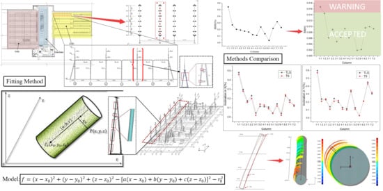
3.2. Cylinder Fitting Model

A cylinder fitting model from point clouds is presented here to obtain the parameters of the reference cylinder by applying the least square error minimization method [29,30] to the data acquired by TLS. According to the geometric characteristic of a cylindrical surface, the distance from the point on the cylindrical surface to its centerline is equal to radius $r_0$, given that $P\left(x,y,z\right)$ is a point on the cylindrical surface, $P_0\left(x_0,y_0,z_0\right)$ is a point on the cylinder axis, $\left(a,b,c\right)$ is the axis vector of the cylinder, and $r_0$ is the radius of the cylinder. Considering the distance from any point on the cylindrical surface to its axis that is equal to radius $r_0$, the equation of the cylinder model can be written as:

$${\left(x-x_0\right)}^2+{\left(y-y_0\right)}^2+{\left(z-z_0\right)}^2-{\left[a\left(x-x_0\right)+b\left(y-y_0\right)+c\left(z-z_0\right)\right]}^2=r_0^2.$$

(3)

By solving the values of seven parameters in Equation (3), a cylinder model can be uniquely determined.

To obtain accurate solution, two essential steps can be used to perform the process of cylinder fitting. The first step is to determine the initial values of the cylindrical model, and the second is to establish error equation to solve the parameters. The solution algorithm combines principal component analysis (PCA) [31] and least square method to determine the initial values of seven cylindrical model parameters, which are cylinder axis vector $\left(a,b,c\right)$, a point $P_{0 }\left(x_0,y_0,z_0\right)$ on the cylinder axis, and radius $r_0$ of the cylinder. Figure 2 illustrates the parametric model of the fitting cylinder.

3.2.1. Determine the Initial Values of the Cylindrical Model

First, the nearest neighbors of a point on the cylindrical surface are randomly searched to serve as the input data for fitting into a plane. Second, the unit normal vector of a point can be obtained by normalizing the plane normal vector simultaneously. With the same principle, the unit normal vector of each point on the cylindrical surface can be gained successively through the normalization process. Third, the unit normal vector of each point is a candidate point, from which is fitted into a plane to further obtain the plane normal vector, which is the initial value of the cylinder axis vector $\left(a,b,c\right)$. In this step, PCA is implemented for obtaining the solution of the equation.

Fourth, the coordinate transformation of the cylinder is conducted to ensure that the axis vector $\left(a,b,c\right)$ of the cylinder is transformed into a reference system parallel to the Z-axis. Last, the (x, y) coordinates of the points on the cylinder surface can be formed into a planar circle. Thus, these planar coordinates can be collectively applied to fit a circle signified as $\left(x_0,y_0,z_0\right)$ and radius $r_0$.

3.2.2. Establish Error Equation

As stated above, the error equation can be constructed as follows:

$$f={\left(x-x_0\right)}^2+{\left(y-y_0\right)}^2+{\left(z-z_0\right)}^2-{\left[a\left(x-x_0\right)+b\left(y-y_0\right)+c\left(z-z_0\right)\right]}^2-r_0^2$$

(4)

Rewrite Equation (4) as:

$$f=\{{\left(x-x_0\right)}^2+{\left(y-y_0\right)}^2+{\left(z-z_0\right)}^2-{\left[a\left(x-x_0\right)+b\left(y-y_0\right)+c\left(z-z_0\right)\right]}^2-r_0^2\}/2$$

(5)

The value $f$ can be linearized as:

$$f=f_0+\frac{\partial f}{\partial x_0}{x}_0+\frac{\partial f}{\partial y_0}{y}_0+\frac{\partial f}{\partial z_0}{z}_0+\frac{\partial f}{\partial a}a+\frac{\partial f}{\partial b}b+\frac{\partial f}{\partial c}c+\frac{\partial f}{\partial r}r$$

(6)

Thus, error equation can be expressed as:

$$V=f_0+\frac{\partial f}{\partial x_0}{x}_0+\frac{\partial f}{\partial y_0}{y}_0+\frac{\partial f}{\partial z_0}{z}_0+\frac{\partial f}{\partial a}a+\frac{\partial f}{\partial b}b+\frac{\partial f}{\partial c}c+\frac{\partial f}{\partial r}r ,$$

(7)

where $f_0$ is defined as:

$$f_0=\{{\left(x-x_0^0\right)}^2+{\left(y-y_0^0\right)}^2+{\left(z-z_0^0\right)}^2-{\left[a^0\left(x-x_0^0\right)+b^0\left(y-y_0^0\right)+c^0\left(z-z_0^0\right)\right]}^2-r_0^2\}/2.$$

The least square method is adopted here to solve the equation $\mathrm{AX}=0$, which means to compute the value of eigenvector corresponding to the minimum eigenvalue of A^TA. The solution is a typical course of iteration. In each iterative process, the initial data of the iteration is equal to the value of the previous iteration plus the correction. When the correction is small enough to meet the required redundancy, the course of iteration will be exited immediately. The pipeline of the algorithm is displayed in Figure 3.

3.2.3. Standard Deviation

Standard deviation can reflect the dispersion degree of a dataset. It also indicates how far observations are from the average. Standard deviation is clearly affected by the extreme value. The smaller the standard deviation is, the more aggregated the data are; conversely, the larger the standard deviation is, the more discrete the data are. Therefore, standard deviation can be used to represent the average deviation level of the distance from each point of the cylindrical surface to the centerline and the distance that is theoretically equal to the radius of the cylinder. Herein, standard deviation is computed to reflect the degree of deformation of each fitted cylinder point to the centerline. The equation of standard deviation can be written as follows:

$$\sigma =\sqrt{\frac{{{\displaystyle \sum }}_{i=1}^N{\left(x_i-\overline{x}\right)}^2}{N}},$$

(8)

where $x_i$ is the distance from a surface point to the centerline of the cylinder,$\overline{x}$ represents the means value of the distance, and $N$ is the number of points.

4. Experimental Setup

To evaluate the performance of the proposed method, an experiment was conducted on the transformer substation composed of steel structures, which have been in service for 15 years. Figure 4 illustrates the layout of the transformer substation. The steel frame areas have three parts, namely, 500 Kv steel frame area, main steel frame area, and 220 Kv steel frame area. The experiment was implemented in the area of 220 Kv, and the distance between the longitudinal outlet frame and the intermediate frame is 23–32.5 m. Each frame is composed of seven A-shaped frame columns (end braces are set on the side columns) and six steel frame beams. Among them, the lightning rod with a 5 m height is installed on the top of the column with an even number, and the spacing of each A-shaped frame column is 13,000 mm. Meanwhile, the A-shaped column is composed of two cylindrical legs, and the length between the bottoms of cylindrical legs is 3000 mm.

Before scanning, the planning is quite critical to ensure that each cylindrical steel structure to be scanned is at least half to provide sufficient data for the fitting process. In the experiment, the scan planning and scanner working site is illustrated in Figure 5. The red triangle represents the position of scanning, whereas the black circle represents the location of the cylindrical steel structure. According to the layout of the scan planning, each cylindrical steel structure in the area can be scanned at least twice in different directions to guarantee the data collected sufficiently. At the same time, the data collected from the different directions can be applied to make a comparison to ensure the accuracy of the results.

Table 1. Scanner specification.

3D Scanner	FARO FocusS 350
Type	phase-shift
Range (m)	350
Accuracy (single measurement) mm	1@25 m
Measuring speed (point per second)	976 thousand
Vertical range	300°
Horizontal range	360°
GPS	Built-in
Camera	Built-in

shows the specification of the scanner.

Taking an A-shaped frame with two columns as the sample to test the proposed method, the point clouds are shown in Figure 6. The number of point clouds in Column 3-1 (left) is 43,811, whereas that of point clouds in Column 3-2 (right) is 42,495. To avoid the impact of point clouds at support joints and welded junctions (displayed in Figure 6), the fitting point clouds are selected manually as large as possible to avoid the influence of interference data. In the course of data selection, some subsidiary facilities, such as the climbing ladder mounted on the steel column as the data show in cylinder 3-2, can also be excluded in the fitting on the basis of manual selection.

After data selection, the proposed method is applied to fit the selected point clouds and calculate the standard deviation of point clouds to the centerline of the cylinder. Figure 7 presents the piecewise fitting result of one cylindrical leg of the A-shaped column. Table 1 shows the corresponding standard deviations.

Table 2. Fitting results.

Number of Columns	Number of Points	Radius (m)	Standard Deviation (m)
1-1	43,694	0.2384	0.0167
1-2	42,171	0.2387	0.0145
2-1	42,213	0.2407	0.0062
2-2	42,590	0.2408	0.0090
3-1	43,811	0.2398	0.0049
3-2	42,495	0.2405	0.0064
4-1	42,121	0.2424	0.0094
4-2	42,380	0.2379	0.0062
5-1	43,105	0.2384	0.0082
5-2	42,570	0.2390	0.0019
6-1	41,134	0.2408	0.0022
6-2	41,747	0.2371	0.0096
7-1	42,367	0.2393	0.0100
7-2	42,579	0.2397	0.0093

presents that according to the same selection principle, the number of point clouds in each column is similar. Due to the construction error, the fitting radius fluctuates around the design value (r = 0.24 m). According to the deviation value, the deviation distribution diagram of the columns is drawn in Figure 8. Most of the standard deviations are between the intervals of 0.005 m and 0.01 m, and only two columns have deviation values greater than the interval. Meanwhile, Columns 5-2 and 6-1 have smaller deviation values, suggesting that the deformations are quite small in both columns. Conversely, the deviation values of Columns 1-1 and 1-2 in Table 2 signify that the deformations are larger than others.

The data in Figure 8 indicate that Column 1-1 has the largest standard deviation among others, which means that the point clouds of Column 1-1 are discrete. At the same time, the standard deviation of Column 1-1 implies that the average deviation level of the distance from each point of the cylinder surface to the centerline is higher than that of others. That is, Column 1-1 has the largest deformation among others.

4.1. Calculation of Inclination by Cylinder Fitting

Given that the value of standard deviation implies the deviation level of the point clouds to the centerline, the real posture of the column is still unknown. Therefore, ensuring whether deformation within the specification is impossible. However, calculating the inclination of the column is quite necessary to help analyze the deformation in different directions. After piecewise fitting the point clouds, as illustrated in Figure 2, the center coordinates of the bottom circle of each fitted cylinder can be obtained easily. However, the obtained coordinates are in the local coordinate system and thus cannot be directly used to compute inclination to represent deformation in the global coordinate system. Coordinate transformation must be implemented first to transform the coordinates into the global coordinate system. Given that the scanner is always level during scanning, coordinate transformation is established by rotating in the $XOY$ plane, but the conversion process is no longer elaborated in this study.

After coordinate transformation, the inclination of each column section can be computed using Equations (1) and (2) with converted center coordinates. The inclinations in the X and Y directions are represented in Figure 9. The left value means the inclination of each section (from the measuring point to the bottom point), whereas the right value is the coordinates of each measuring point. The overall inclination means the inclination rate of the highest point to the lowest point in each direction. The discrepancy of inclination between different sections should be consistent in theory, but due to the existence of deformation, a discrepancy exists between them. Therefore, the maximum axial inclination means the maximum discrepancy of the sectional inclinations in the same direction. According to the principle, the inclinations of each column are calculated in

Table 3. Inclination of each column by the proposed method.

Number of Columns	Overall Inclination (%)		Maximum Axial Inclination (%)
	X	Y	X	Y	RMSE
1-1	−10.216	0.138	0.482	0.598	0.543
1-2	10.238	−0.321	0.299	0.239	0.271
2-1	−10.139	0.204	0.175	0.23	0.204
2-2	10.243	−0.222	0.232	0.142	0.192
3-1	−10.176	0.168	0.045	0.245	0.176
3-2	10.134	−0.078	0.116	0.200	0.163
4-1	−10.309	0.212	0.113	0.132	0.123
4-2	10.066	−0.133	0.108	0.117	0.113
5-1	−10.244	0.059	0.045	0.334	0.238
5-2	10.091	−0.129	0.143	0.129	0.136
6-1	−10.154	−0.011	0.041	0.030	0.036
6-2	10.231	−0.236	0.228	0.212	0.220
7-1	−10.295	−0.002	0.184	0.451	0.318
7-2	10.099	−0.051	0.120	0.304	0.231

.

In Table 3, the maximum axial inclination represents the maximum discrepancy of inclination between different sections and can be used to represent the maximum deformation of the column. Column 1-1 has the largest maximum axial inclinations in X (0.482%) and Y (0.598%) directions, and the deformation values are coincident with its standard deviation. RMSE is computed to measure the inclination degree of direction. Figure 10 illustrates that Column 1-1 has the largest RMSE, whereas Column 6-1 has the lowest RMSE. Column 7-1, as the side column, has the second largest RMSE. Therefore, in terms of the whole structures, side columns at both ends have larger deformation values than the middle ones; the deformation directions are also the same with each other, both tilting in the positive directions of X and Y at the position of side columns. The trend is consistent with the standard deviation analysis. Meanwhile, the column with a small standard deviation almost has a small deformation value in each direction, as illustrated in Figure 8 and Figure 10.

4.2. Methods Comparison

With respect to the site detection conditions, SOKA total station (TS) of SET1130R3 (±1’) is used as a conventional instrument to collect the data of the legs of A-shaped frame columns within the detection range. Such collection is based on the first-level measurement requirements of deformation observation. According to the power industry standard (DL/T5218-2005) of “technical code for design of 220–500 kV substation” for A-shaped frame columns, the allowable deformation limit inner plane is 5‰H (H is the height from the column bottom to the test point), and the allowable deflection limit out of plane (without brace) is 10‰H.

Table 4. Inclinations of each column by total station.

Number of Columns	Overall Inclination (%)		Maximum Axial Inclination (%)
	X	Y	X	Y	RMSE
1-1	−10.18	0.12	0.46	0.57	0.52
1-2	10.21	−0.31	0.28	0.21	0.25
2-1	−10.12	0.18	0.16	0.24	0.20
2-2	10.23	−0.21	0.20	0.11	0.16
3-1	−10.18	0.18	0.02	0.21	0.15
3-2	10.11	−0.08	0.14	0.22	0.18
4-1	−10.29	0.19	0.13	0.11	0.12
4-2	10.05	−0.11	0.09	0.10	0.10
5-1	−10.21	0.05	0.04	0.35	0.25
5-2	10.11	−0.11	0.12	0.11	0.12
6-1	−10.13	−0.02	0.02	0.03	0.03
6-2	10.21	−0.23	0.24	0.21	0.23
7-1	−10.31	−0.01	0.16	0.43	0.32
7-2	10.11	−0.05	0.13	0.32	0.24

shows the deformation detection results of each frame column (including construction error).

Table 4 shows that Column1-1 has the largest axial inclination in the Y direction, which has exceeded the limit of DL/T5218-2005 requirement. This trend is the same as the proposed method based on the point clouds. Figure 11 displays the comparison of two methods in different directions. As illustrated, the deformation results of columns are quite similar in both directions. In the X direction, the largest deflection occurs in Column 1-1 with two different methods, but the values are still under the limit required in the standard of DL/T5218-2005, which asks for the allowable deflection limit (without brace), that is, 10‰H. In the Y direction, the largest inclinations in the two methods are 0.598% and 0.57%. Both exceed the requirement of the standard of DL/T5218-2005 that the allowable deformation limit is 5‰H, which means Column 1-1 has a severe safety status. Importantly, the largest inclination values corresponding to the largest standard deviation, which can be implied in Figure 8 and Figure 10, indicate that the standard deviation can be used to represent the deformation degree of each column. Figure 11 also shows that the values of TS is a little bit more accurate than those of TLS, but the gap between the two is quite small in each column. Thus, TLS can completely replace TS in terms of efficiency and accuracy in practice. Moreover, the point clouds obtained by TLS are more comprehensive than the data of TS, which can be used to analyze the entire deformation of columns.

4.3. Global Deformation Analysis

To directly reflect the deviation size, the deviation can be visualized by color maps. Herein, to ensure the actual posture of the column scanned by TLS, Column1-1 is selected as an example for further analysis to ascertain its actual deflection. In color maps, cool colors represent the deviation far from the interior of the fitting model, whereas warm colors indicate the deviation far from the outside of the fitting model. Specifically, the green color means the deviation is small enough to be close to the fitting model. As shown in Figure 12a, the color differences clearly indicate the deviation in contrast to the fitting column from the bottom to the top, and a total of four sections of deformation colors shown in the point clouds exist. The first section is [0 m, 6.4 m]; here, the radial deformation is apparently small and mostly colored with green; only a tiny part of points around 0 m have an outward deviation within 2 cm. The second section is [6.4 m, 10.7 m]; an inward deviation is observed with 2 cm arched inside the fitting model. The third section is [10.7 m, 15.2 m]; the posture of the point clouds returns to normal colored with green compared with the reference. The fourth section is [15.2 m, 26.3 m]; with the increase in height, the point clouds have gradual increasing outward deflection with almost 11 cm radial deviation at the end of the column. The sectional deformations of point clouds to the fitting model from the top view can be drawn in Figure 12b, which clearly reflects the variation of each section in different directions.

From the analysis of the deformation with color maps, the global deformation of steel structure columns is clearly reflected by the point clouds compared with the fitting model. Meanwhile, the deformation of different parts can be accurately calculated to determine the location and the size of the change. Through the analysis of seven pairs of columns, the threshold of standard deviation in the experiment is set as 0.015 m, corresponding to the limit of the allowable deformation listed in the standard of DL/T5218-2005, which can be adopted in the proposed method to signify the limit of allowable deformation.

5. Conclusions

This study provides an effective approach to fitting the cylinder model for A-shaped specific steel structures from dense point clouds collected by TLS. A deformation analysis is also conducted on the basis of the fitted model. In this study, the method for the deformation monitoring of a cylindrical steel structure is presented on the basis of the dense point clouds collected by TLS. Meanwhile, scan planning before data acquirement is emphasized in advance to ensure that each cylindrical steel structure is covered (at least half) to provide sufficient data for fitting. The piecewise cylinder fitting method is also put forward in this study to fit the point clouds collected at one time for computing the relative inclination of the cylindrical steel structure. Moreover, standard deviation is adopted as a measure to evaluate the degree of structure deformation.

The accuracy and reliability of the proposed model are evaluated by taking an A-shaped column composed of two cylindrical legs in the actual substation as an example. After data selection, the proposed method is applied to fit the selected point clouds and calculate the standard deviation of point clouds to the centerline of the cylinder. Through the analysis of seven pairs of columns, the threshold of standard deviation in the experiment is set as 0.015 m, corresponding to the limit of the allowable deformation listed in the standard of DL/T5218-2005, which is used in the proposed method to signify the limit of allowable deformation.

Furthermore, two methods in different directions are compared in the experiment. The deformation results of the columns are quite similar in both directions. In the X direction of the global coordinate system, the largest deflection occurs in Column 1-1 with two different methods, but the values are still under the limit requirement in the standard. In the Y direction, the largest inclinations in the two methods are 0.598% and 0.57%. Both values exceed the requirement of DL/T5218-2005 that the allowable deformation limit is 5‰H. Moreover, the largest inclination values correspond to the largest standard deviation in the proposed method.

Color maps are used to further illustrate the actual deformation of experimental structures in different directions. Through an analysis, a total of four sectional deformations marked with different colors are found, and the largest deformation is 10.93 cm at the end of the column from the top view of Column1-1. Meanwhile, the sectional deformations of point clouds to the fitting model from the top view are clearly drawn to reflect the variation of each section in different directions.