Article

Sentinel-2 Remote Sensed Image Classification with Patchwise Trained ConvNets for Grassland Habitat Discrimination

1
Institute of Atmospheric Pollution Research (IIA), National Research Council (CNR), Via Salaria Km 29 300, 00015 Monterotondo, Italy
2
Department of Civil Engineering and Computer Science Engineering, University of Rome “Tor Vergata”, Via del Politecnico 1, 00133 Rome, Italy
3
Institute of Atmospheric Pollution Research (IIA), National Research Council (CNR), c/o Interateneo Physics Department, Via Amendola 173, 70126 Bari, Italy
4
Department of Biology—Botanical Garden Museum, University of Bari, Via Orabona 4, 70125 Bari, Italy
*
Author to whom correspondence should be addressed.
Remote Sens. 2021, 13(12), 2276; https://doi.org/10.3390/rs13122276
Submission received: 23 April 2021 / Revised: 7 June 2021 / Accepted: 9 June 2021 / Published: 10 June 2021
(This article belongs to the Special Issue Deep Learning for Remote Sensing Image Classification)

Abstract

:
The present study focuses on the use of Convolutional Neural Networks (CNN or ConvNet) to classify a multi-seasonal dataset of Sentinel-2 images to discriminate four grassland habitats in the “Murgia Alta” protected site. To this end, we compared two approaches differing only by the first layer machinery, which, in one case, is instantiated as a fully-connected layer and, in the other case, results in a ConvNet equipped with kernels covering the whole input (wide-kernel ConvNet). A patchwise approach, tessellating training reference data in square patches, was adopted. Besides assessing the effectiveness of ConvNets with patched multispectral data, we analyzed how the information needed for classification spreads to patterns over convex sets of pixels. Our results show that: (a) with an F1-score of around 97% (5 × 5 patch size), ConvNets provides an excellent tool for patch-based pattern recognition with multispectral input data without requiring special feature extraction; (b) the information spreads over the limit of a single pixel: the performance of the network increases until 5 × 5 patch sizes are used and then ConvNet performance starts decreasing.

Graphical Abstract

1. Introduction

An increased interest in classification methods has emerged in the last three decades, receiving considerable research attention especially in Earth Observation (EO) applications through land cover and habitat mapping by means of both optical and radar satellite images.
To this end, an enormous amount of studies has been carried out through the years in an attempt to improve classification accuracy, as extensively summarized by [1], and a variety of satellite data have become available based on a free access policy.
One of the most challenging applications of remote sensing is the monitoring of natural and semi-natural grassland ecosystems, representing one of the largest landscape units in the terrestrial system [2]. EO data and automatic classification techniques can support the mapping of grassland ecosystems. However, the spectral signature of such ecosystems can be rather complex due to the heterogeneous nature of the habitats composing them [2,3] and, despite recent successful attempts, grasslands mapping is still regarded as challenging [4].
Some studies have already addressed natural and semi-natural grassland ecosystems monitoring at medium–high spatial resolution, exploiting both optical and SAR data by using machine learning approaches [5,6,7,8,9,10,11,12,13]. In particular, a Support Vector Machine (SVM) classifier was used to analyze, both separately and in combination, a series of four optical (5 to 30 m) and five SAR images (12 m), for discriminating natural grasslands from croplands in areas affected by frequent clouds [5]. SVM was also used to distinguish seven grassland habitats by integrating an inter-annual time series of RapidEye and TerraSAR-X images [2]. Xu et al. (2019) [6] focused on the classification of different grassland types from multi-temporal Landsat images, in combination with a 30 m DTM. The authors used both SVM and Random Forest (RF) object-based classifiers. The overall classification accuracy exceeded 90% using both classifiers, and the classification accuracy of the grassland types considered ranged from 61.64% to 98.71%. The data-driven RF classifier was used for mapping different types of grassland communities by analyzing Landsat and Worldview-2 data [7]. Buck et al. (2015) [8] also analyzed three multi-temporal RapidEye images for mapping three Natura 2000 grassland habitats, including Type_1 habitat, an “intensive grasslands” class, and two additional crop classes in Germany. They compared the results from a Maximum Likelihood (ML) classifier with the ones from a Support Vector Machine (SVM). Zlinszky et al. (2014) [9] used LIght Detection And Ranging (LIDAR) data from two different aerial campaigns for mapping grassland habitats in Hungary by adopting the Random Forest (RF) classifier. Marcinkowska-Ochtyra et al. (2019) [10] analyzed three multi-temporal hyperspectral images combined with Digital Terrain Model (DTM) information for mapping three grassland habitats, including Type_1 habitat, in Poland, by applying an RF classifier. Rapinel et al. (2019) [11] compared the results obtained by SVM and RF to map seven floodplain grassland plant communities by using intra-annual Sentinel-2 time series or a mono-temporal dataset. The results reported identify SVM as the better of the two classifiers. Fauvel et al. (2020) [12] combined a time series of NDVI index from Sentinel-2 with polarization data from Sentinel-1 SAR time series for mapping grassland plant diversity in France. They compared five conventional machine learning algorithms, i.e., linear regression, K nearest neighbors, Kernel Ridge Regression (KRR), Random Forest (RF) and Gaussian Process (GP), finding RF to be the best performing in predicting grassland plant diversity. Tarantino et al. (2021) [13] considered the same input dataset and training/validation reference data of the present work by using an SVM classifier.
Focusing on the supervised methods, a prominent role has been assumed by Artificial Neural Networks (ANNs) as one of the most suitable techniques dealing especially with multispectral image data [14]. ANNs are a collection of connected and tunable units, known as nodes or neurons, which are able to propagate a signal from an input unit, also called an input layer, to an output unit, the output layer, through one or more intermediate layers, known as hidden layers. ANNs are implemented using non-statistical algorithms and, for this reason, are generally described as nonparametric. They do not require any assumptions about the statistical distribution of the data and their performances depend on how correctly they have been trained about regularities of the training data in order to construct rules that can be extended to the unknown data. ANN architecture and parameters, such as the learning rate, are defined by the user following heuristics. The authors of [15] portray a rich description of the use of ANNs in remote sensing. Taking into account ANNs’ sensitivity [16,17] investigated the effects of changing the numbers of network nodes in the input and hidden layers, in order to create a more compact network without loss of classification accuracy, and the use of different rates of network learning leading to a more rapid convergence and better classification of land cover and habitat.
With the advent of Big Data, the number of ANN hidden layers has rapidly grown and Deep Learning (DL) originated [18]. Convolutional Neural Networks (CNNs or ConvNet) are one of the subcategories of neural networks evolved from Multilayer Perceptron (MLP) [19]. CNNs have been largely used in remote sensing tasks in the last years, including classification [20,21,22,23,24,25], and achieve the best performances among other machine learning approaches such as Support Vector Machine (SVM), Random Forest (RF) and Decision Tree (DT) [26,27,28].
The present study focuses on the use of a CNN to classify a multi-seasonal dataset of Sentinel-2 images for discrimination of four grassland habitats in the “Murgia Alta” protected site.
Although efforts have been made on the automatic mapping of grassland habitats by means of machine learning techniques, to the best of our knowledge there are no publications that have explored the use of CNN for this purpose.
Thus, the goal of the present work is to assess the performance of a patchwise-trained ConvNet, using multispectral data as input, for a grassland habitats discrimination problem. Two experiments were carried out: (a) evaluating how the information, needed for classification by a ConvNet spreads over convex sets of reference pixels, split into patches, varying the size of square input patches; (b) assessing the quality of a patchwise-trained, ConvNet-based pattern detector fed in input with multispectral data applied to grassland habitats mapping. Furthermore, the performance of a ConvNet was compared with that of a corresponding fully connected architecture network.

2. Materials and Methods

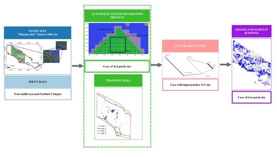
2.1. Study Area and Grassland Habitats Characterization

The study area is located in the Mediterranean basin within the Apulia region, Southern Italy. The area (red boundary, Figure 1) covers nearly 800 km2 within the Natura 2000 “Murgia Alta” protected area (IT9120007) (black boundary, Figure 1). This is a Site of community importance and in addition a Special Protection Area that has been included in a National Park since 2004.
The altitude of the area ranges from 285 to 680 meters above sea level. The site is characterized by a typical Mediterranean agro-pastoral landscape with millennial land-use history mainly occupied by semi-natural rocky dry grasslands, traditionally used as extensive pastures [29]. In “Murgia Alta”, the semi-natural grassland ecosystem hosts numerous endemic, rare or trans-Adriatic distribution species [30]. This area is considered of crucial importance for the conservation of wildlife and priority species [31].
During the last three decades, this unique ecosystem has been exposed to tremendous impacts and an accelerated processes of habitat degradation, fragmentation and biotic contamination (i.e., woody encroachment), both within and next to its borders, on local biodiversity, due to both agricultural intensification (transformation of grassland pastures into agricultural cereal crops intensification) and land abandonment. Furthermore, the long-term below-average rainfall (climate change), the increasing of either legal and illegal mining activities or wind farms infrastructures and arson [32,33] and the spread of invasive species contribute to the threat to the ecosystem, which is in danger of destruction [34,35].
The four grassland habitat types considered in the study area are listed and described in Table 1 according to Annex I of the European Habitat Directive [36] and the EUNIS habitat taxonomies [37].

2.2. Data Availability

2.2.1. Ground Truth

To obtain a set of reference polygons, georeferenced surveys of the vegetation were carried out using the phytosociological method of the Sigmatista School in Zurich-Montpellier [38] based on the complete floristic composition for the plant community investigated. This approach is recognized at the EU level [39,40] since it allows a precise diagnosis for many habitats of the Directive and in particular for grassland habitats. For our work, the sampling was first stratified, i.e., the relevés were carried out randomly in areas previously identified on the basis of their physiognomic and structural homogeneity. Then, after a multivariate numerical classification by using the coverage values transformed according to the scale proposed by van der Maarel (1979) [41], the different plant community types were identified and consequently attributed to the habitats of both the EU Directive [39], based on the “Interpretation Manual of European Union habitats”, and the “Manuale Italiano di Interpretazione degli Habitats” [42,43]. Thereafter, a polygon related to a homogenous area around each relevés was identified by a visual interpretation of the available orthophoto (2018). The data reported in Table 1 are related to four different habitat grasslands classes, which correspond to the same Land Cover (LC) class of semi-natural grasslands.
Due to the highly time-consuming process involved in the recognition and collection of the ground data, the reference polygons dataset resulted in having a rather small cardinality and a high asymmetry mainly among the different classes, with a lower presence of habitats characterized by small and highly fragmented patches.
Figure 2 shows some close-ups of ground truth polygons overlaid on an orthophoto (2 m spatial resolution), for the different habitat classes investigated.
For each class, the percentage of 75% (54,725 pixels) from the available ground truth samples was randomly selected for training and testing. Validation of the classifier was performed using the 100% (73,386) of ground truth data in a k-fold procedure. Figure 3 shows ground reference samples distribution for each grassland habitat class.

2.2.2. Satellite Data

For the year 2018, four multi-seasonal Sentinel-2A images were freely downloaded from the United States Geological Survey (USGS) EarthExplorer portal [44], selecting images with less than 10% cloud cover on the study area. Table 2 reports the date of acquisition for each image.
The entire study area was covered by the tile 33TXF and the orbit R036 was considered. Level-2A surface reflectance products were downloaded for the images.
Sentinel-2 images include four spectral bands at 10 m spatial resolution in blue (B2: 458–523 nm), green (B3: 543–578 nm), red (B4: 650–680 nm) and NIR (B8: 785–899 nm) spectra. They also contain six bands at 20 m spatial resolution in red-edge (B5: 698–713 nm; B6: 733–748 nm; B7: 773–793 nm), NIR (narrow) (B8A: 855–875 nm) and Short Wave Infra-Red (SWIR) (B11: 1565–1655 nm; B12: 2100–2280 nm) spectra. Thus, in our work, 10 spectral bands per each image were investigated. The three atmospheric bands (B1, B9, and B10) at 60 m spatial resolution were excluded from the analysis. Each image was cropped according to the boundary of the area of interest, and then all of the images were stacked, obtaining a single raster file of 40 layers. Only those pixels belonging to a pre-existing grassland layer, obtained by applying the automatic procedure proposed in [13], were considered.

2.3. Algorithm for Habitat Mapping

To discriminate between the four grasslands habitats listed in Table 1, a CNN classifier was adopted to investigate the performance of such a classifier for approaching an application characterized by a complex reference dataset, as detailed in Section 2.2.1.

2.3.1. CNN Classifier Configuration

CNNs are feedforward neural networks and are characterized by sparse connectivity: neurons of adjacent layers are collected by only local connections. In addition, each neuron in a layer shares the same weights and bias. CNNs consist of a series of convolutional, pooling, and nonlinear activation functions. They select features automatically by applying multiple filters (called convolutional kernels) on the input images in the form of multidimensional arrays (i.e., image patches), and learn to select the ones that are necessary for the images’ proper classification [45]. Features in a rectangle neighborhood are then aggregated into one feature by the pooling layer [46]. CNN parameters are divided into hyper-parameters and non-hyper-parameters: the first include input size, convolution kernel size, number of convolution kernels, pooling kernel size, and learning rate; the second refer to the weights of the hidden layers that are adjusted during the training by using a Back Propagation (BP) algorithm [47]. However, no definite rules have been codified for the optimization of the CNN parameters, whereby the choice of their setting depends on the user experience [48,49]. CNNs need large training image datasets [50], which are usually not available; hence, to correctly train large architectures pre-trained CNNs [51,52,53,54,55] or segmentation techniques, such as transfer learning [56,57] and active learning [58], are used to overcome this problem.
The most widespread strategy in land cover classification is based on the use of patches by applying moving windows with a fixed size on each pixel [59,60,61,62,63]. By varying input and output network configurations through the patch sizes, classification accuracy and computational cost can be adjusted according to the scenario that has to be classified.
CNNs are most frequently used to classify image data with high spatial resolution (especially up to 10 m) thanks to their ability to extract high-level feature information using a single image scene or multisource remote-sensing data [26]. Thus, a CNN was adopted for our study due to the 10 m spatial resolution of multi-temporal Sentinel-2 data considered for the grassland habitat mapping and the possibility to exploit the contextual information contribution by using a per patch approach.
A basic ConvNet for image classification relies on the following architecture: input–conv–pool—Fully Connected (FC) [64], where the main purpose of the pool layer is to reduce the size of the input data [65]. Due to the patch size used in these experiments being small compared to the convolutional kernel sizes usually chosen with ConvNets, the pool layer was removed.
Consequently, the patch-tailored ConvNet architecture adopted in this study is described in Table 3.
In Table 3:
  • The input layer specifies the size of the patches, that in our case is variable between 1 × 1 and 6 × 6, while num_bands (in our case equal to 40) refers the depth of the multispectral Sentinel data;
  • kernel_size is an integer specifying the height and width of the 2D convolution window, whereas depth (equal to 32 in our case) is the dimensionality of the output space (i.e., the number of output filters in the convolution). Such value was determined in the meta-parameter tuning procedure as an effective compromise between the architecture complexity and the learning curve convergence;
  • output_size (equal to 128 in our case) is the number of output neurons of the first FC layer;
  • num_classes (equal to 4 in our case) is the number of output neurons of the latest FC layer.
In order to prevent the network from overfitting, two dropout layers [68] were added before each of the two FC layers.
In addition to the settings in Table 3, for all layers, the model used biases initialized at zero and a Gloriot uniform weight initializer [69]. This method was implemented according to Keras [70].
Figure 4 shows the adopted network architecture in terms of units and connection for the case with input patches of 5 × 5 size.
The architecture of our network has been designed to comply with our goals: (1) show the effectiveness of a CNN-based approach with our data; (2) show how the information spreads over multiple multispectral pixels. The selected number of units represents a compromise between the computational effectiveness and performance of the network.
The input multispectral dataset includes 40 bands as fully detailed in Section 2.2.2.
To generate the patch-based dataset, the set of polygons was tessellated, embedding the on-site verified pixels in square patches. Patches of multispectral pixels with 1 × 1, 2 × 2, 3 × 3, 4 × 4, 5 × 5, and 6 × 6 sizes were generated by using the procedure described above, as shown in Figure 5.
In Figure 5, the blue areas highlight the masked pixels (i.e., pixels set to zero to prevent their contribution), the light purple areas show the unmasked pixels, the green areas show the closed sets delimiting the ground truth, the light yellow lines highlight overlapping patches, and the black thick box represents a 4 × 4 patch size. A pixel is considered as part of a patch if its center lies inside a ground truth polygon. The x and y axes show the pixel coordinates.

2.3.2. Experimental Setting

As stated above, besides generally assessing the effectiveness of ConvNets with patched multispectral data, the purpose of the present study was to determine how the information needed for classification spreads to patterns over convex sets of pixels. To this end, six datasets of square patches with 1 × 1, 2 × 2, 3 × 3, 4 × 4, 5 × 5, and 6 × 6 sizes were created. Due to the spatial layout of the data, the 6 × 6 size is the maximum one allowed by the dataset in order to avoid the Type_1 patches disappearing.
Table 4 shows the patch distribution with respect to the classes.
The data in Table 4 represent the number of patches generated with different sizes for each grassland habitat class. Every pixel within the patches covers an area of 10 × 10 meters on the ground.
As evident by inspecting Table 4, the dataset grow more and more unbalanced with the patch size. To restore balance, the classes have been weighted in the loss function according to the following equation:
w i j f r e q j f r e q i × k j k f r e q j
where freqi and wi are, respectively, the frequency and weight of the specific class.
To assess the quality of a ConvNet in a grassland habitats discrimination problem two experiments were carried out:
A.
Evaluating how the information needed for classification spreads over multiple multi-spectral pixels varying the size of square input patches to the ConvNet (Information Localization). In detail, in our setting the kernel size of the ConvNet (kernel_size × kernel_size) was grown linearly with the patch size. As no padding was set up, the FC part of the network remained unchanged while the convolution kernel increased and took charge of the pattern recognition task.
B.
Comparing the performance of a ConvNet with that of a corresponding FC architecture network. For fair comparison, the FC was set up by leaving untouched the original ConvNet with the exception of the kernel size of the convolutional layer, which, in this second instance, has been kept to a 1 × 1 size.
Our CNN settings include:
  • A total of 120 epochs with a batch size of 32 and 1000 steps per epoch;
  • A kernel size equal to the size of the input patches;
  • An Adadelta optimizer with: (a) 0.001 as learning rate; (b) a decay rate of 0.95; (c) a stability factor of 1 × 10⁻⁷.
The adopted Keras [70] framework and the experiments were performed on an Ubuntu 18.04 Lenovo ThinkStation P520.
Figure 6 shows the flowchart of the different steps implemented in our experiment.

2.3.3. Accuracy Assessment

Due to the small size, the scarcity and the unbalanced character of the dataset, tessellating our ground truth polygons has proven progressively challenging when dealing with patches of increasing size. Therefore, at first, we split the dataset into two sets, one for training and testing (to perform hyperparameters tuning) and one for validation.
Once the hyperparameters had been tuned, we performed a final validation by stratified k-fold (with k = 3) using the whole dataset: the dataset was therefore randomly split three times into a training set and a test set, and the final test score was an average of the performance during the three combined training and test procedures. Stratified k-fold provides train/validation indices to split data in train/validation sets [71]. This cross-validation object is a variation of k-fold preserving the percentage of samples for each class. As our class distribution was strongly uneven, the performance of our system was measured with the F1-score metric, as detailed in the following formulas:
Precision = TP TP + FP Recall = TP TP + FN F 1 score = 2 × Precision × Recall Precision + Recall
where:
  • TP = True Positive (number of samples correctly assigned to a class);
  • FP = False Positive (number of samples incorrectly assigned to a class);
  • FN = False Negative (number of samples of a class incorrectly assigned to another);
  • The F1-score metric performs the harmonic mean of Precision and Recall [72].

3. Results

3.1. Grassland Habitats Characterization

Surface reflectances represent the input features of the classification procedure. They were, therefore, initially analyzed to provide grassland habitats characterization in terms of their spectral and seasonal behaviors. The surface reflectance values were analyzed separately for each season and habitat, resulting in 16 spectral signatures (Figure 7).
It can be noticed that all of the classes exhibited the highest photosynthetic activity in spring, except for Type_3, for which winter represented the peak of the biomass season. This can be explained considering that this habitat is typically located on south-facing slopes. The availability of water, due to precipitation and the presence of not particularly cold temperatures, resulted in reaching photosynthetic activity earlier than the other types. Although Type_1 showed the same seasonality as both Type_2 and Type_4, it differed from them in terms of absolute values of surface reflectance in the rededge and NIR bands in spring. Type_2 and Type_4 habitats showed similar spectral responses for the different seasons. Some differences could be observed only for SWIR bands’ surface reflectances in autumn.
The spatial characterization of the different grassland habitats can be observed hereafter. In Figure 8 the yellow patch 6 × 6 size, overlaid on samples of the different classes of grassland habitat, highlights the higher Type_4 class heterogeneity on the ground compared to the other classes. Hence, as patch size increased, the presence of heterogeneity resulted in a reduced suitability to discriminate that class by the CNN.

3.2. Information Localization

The findings obtained in the first experiment (Section 2.3.2, Experiment A) are reported in Table 5 and shown in Figure 9 and Figure 10.
Figure 9 reports the values of F1-score computed for each of the classes considered for the different input patch sizes considered.
The averaged F1-score (Table 5) increased as the patch size increased to the 5 × 5 size and then showed a slight decrease with 6 × 6 patch size. The explanation of this behavior is twofold: on the one hand, the dataset grows more and more asymmetric by the patch size, which makes it harder to re-balance; on the other hand, the Type_4 class, which is non-specific as it collects all the vegetation types not belonging to the other types, grows more noisy by the patch size and eventually drives the overall behavior. In other words, unlike the other cases, increasing the patch size augments the amount of noise present in the Type_4 patch instead of the amount of information. This fact is highlighted by the per-type F1-score graph (Figure 9).
In Figure 10 the accuracy estimators, i.e., precision (Figure 10a) and recall (Figure 10b), for the different classes vs. the input patch size are plotted.
It is interesting to note that Type_4 displayed a decreasing trend that was slightly different from the other types. This is especially evident in the precision graph, while the decrease in the recall graph is slightly less noticeable. However, the F1-score being the harmonic mean of precision and recall, its decreasing trend is clearly biased by the precision contribution, which, in turn, is determined by a significant variation of FP over the FN. An ideal compromise appears to be suggested by the 5 × 5 patch size with the four habitat types showing similar values both in precision and recall.
The results of the grasslands habitat mappings and the percentage of pixels mapped as the patch size varies can be seen in Figure 11 and Figure 12, respectively.
From the prior knowledge provided by ecologists it is known that the study area is characterized by the presence of 70–80% of the dominant class Type_2 followed by the class Type_4 and then by the presence of a minority of Type_1 and Type_3 classes. Such a distribution can be evaluated, also, from the ground truth samples considered for training (Figure 3). To handle the asymmetric nature of our dataset, we adopted a twofold strategy: first, we balanced the contribution of each class type in the loss function with respect to their frequency; second, we chose F1-score as our metric to balance precision and recall.
Mappings obtained at larger patch sizes (i.e., 5 × 5 or 6 × 6) can be considered more confident with respect to the expected grassland habitats distribution, whereas at smaller patch sizes an overestimation mainly of Type_3 class followed by Type_1 emerged. Those pixels belong to the misclassified Type_2 dominant class. The specific distribution of the mapped pixels varying the patch size can be seen in Figure 12.
The effect of the patch size growing is to increase the percentage of grassland assigned to Type_2 (Figure 12), in agreement with the expected spatial distribution of the four habitats in the study site.

3.3. ConvNet vs. FC Network Performance

Figure 13 shows the results of the second experiment (Section 2.3.2, Experiment B). The fully connected network corresponds to the case of ConvNet with a 1 × 1 patch size.
As seen in Figure 13, the ConvNet-based architecture outperformed the corresponding FC when the size of the input patches grew past 3 × 3. This result is more relevant when the number of parameters used in the two approaches are also compared (Figure 14).
As shown in Figure 14, the number of parameters needed for the FC architecture to approximately match the ConvNets in the 5 × 5 and 6 × 6 cases was more than two times larger.
To evaluate further this aspect we performed an additional experiment reducing the number of parameters of the FC architecture to a size similar to the ConvNet case. To this end, we reduced the depth of the convolution layer from 32 to 12 and fed it with the patches exhibiting the best performance (5 × 5 input patches). This resulted in an architecture with 39,536 parameters for this FC case, to be compared with the performance of the 36,772 parameters of the corresponding ConvNet with a filter kernel of 5 × 5 size. Figure 15 shows the results.
In Figure 15, the F1-scores of the two architectures are further compared with the ConvNet architecture with 3 × 3 patches as input. The FC architecture using 5 × 5 patches (middle column) was outperformed in terms of F1-score by the ConvNet using 5 × 5 patches, which relied on a similar number of parameters (left column). Moreover, it performed slightly worse than the ConvNet case using 3 × 3 patches (right column), which relied on a smaller number of parameters.
This experiment highlights the typical ConvNet ability to leverage the spatial correlation among the pixels: a multi-perceptron (FC) fed with 5 × 5 patches, with a kernel size of 1 × 1, needs ~3 times the number of parameters of a ConvNet to achieve similar performances (although still slightly inferior). Indeed, single-pixel fed networks are also able to exploit spatial correlation; however, unlike Convnets, they are not specifically designed for it, and therefore they need more parameters and more training (Figure 15).

4. Discussion

The present work aimed at assessing the performance of a ConvNet classifier for a grassland habitats discrimination problem. The Mediterranean grassland habitats considered require a highly time-consuming process for the recognition and collection of the ground truth data to be used for training and validation of the classifier. This implies that the reference polygons dataset is characterized by a rather small cardinality and a high asymmetry, mainly for those grassland habitat classes with lower presence on the ground that are characterized by small and highly fragmented patches. Due to the mentioned peculiarities of the specific application, the ability to obtain a reliable mapping for these grassland habitats represent a challenge.
In most previous papers, Type_1, among the set of grassland habitats considered in our work, was detected using different machine learning algorithms. Using a random forest classifier, Zlinsky et al. (2014) [9] obtained User’s Accuracy (UA) and Producer’s Accuracy (PA) values equal to 66.4% and 78.6%, respectively, and Marcinkowska-Ochtyra et al. (2019) [10] obtained an F1-score of 84.5%. Considering SVM classifiers, Buck et al. (2015) [8] obtained an UA lower than 53% and an F1-score of 89.11%. Tarantino et al. (2021) [13] considered the same input dataset and training/validation reference data of the current study using an SVM classifier; lower accuracies for all of the habitat classes resulted. In detail, these authors obtained F1-score values of 89.11%, 97.29%, 72.82%, and 57.81% for Type_1 to Type_4 grassland habitats, respectively. Using ConvNets results appeared encouraging. In our best findings (i.e., 5 × 5 patch size), we obtained F1-scores of 97.00%, 100.00%, 99.33%, and 92.00%, for Type_1 to Type_4 grassland habitats, respectively (Figure 9).
Our work exploited the effectiveness of a CNN in the detection of grassland habitats and its higher suitability to manage such a problem with a training dataset characterized by low cardinality and asymmetry. These limitations were approached by considering tessellating the input dataset with square patches centered around the reference data for each sample. Enlarging the patch size, an increase in accuracy in terms of F1-score for all the classes except Type_4 was registered. This result can be explained considering the essential role of contextual information around each training sample, due to the correlation among pixels. The use of such a per patch approach can be assimilated to an automatic spatial feature extraction. The patch size cannot be increased indefinitely because, as can be observed in Table 4, of the risk of missing the presence of the Type_1 class. Another limitation in the increasing patch size was obtained in the worsening of the accuracy for the Type_4 class. This can be due to the specific heterogeneity of the Type_4 class (Figure 8), which is composed of different grassland communities and, presumably, the higher the patch size, the noisier the informative contribution associated with the patch, which can cause misclassification.
However, observing the overall habitat mapping obtained by using different patch sizes, a reduction of the overestimation areas covered by Type_3 class can be noticed, followed by Type_1, in favor of the dominant habitat Type_2 (Figure 11 and Figure 12). Patch size growth results in a distribution of grassland habitats areas that is quite in agreement with the expected spatial distribution in the study site. Indeed, the “Murgia Alta” site is characterized by a large presence of Type_2 habitat of almost 70–80% and a lower presence of the remaining types. Hence, the use of a variable patch size can be considered a useful approach to take into account the edaphic conditions of the grasslands ecosystem in the study site. Moreover, the combined use of multi-seasonal and multispectral information derived by the four selected satellite images as input to the CNN seems to provide encouraging results in grassland habitat discrimination.
It is well-known that ConvNets are able to exploit eventual correlations among closely located data on a 2D grid by extracting information in a similar way to which 2D non-separable finite impulse response (FIR) filters extract frequency content.
From a theoretical standpoint, the difference between the two approaches examined in this work (1 × 1 patches and N × N patches with N > 1) is highlighted by the formulae in Equation (3):
o u t s p k = F w · i n p u t o u t w k = F i w i · i n p u t i
In Equation (3), the top equation refers to the 1 × 1 patch case (spk, single pixel kernel) while the bottom one refers to ConvNets equipped with wide-kernels (wk) covering a whole patch (with patch size bigger than 1 × 1). In this representation, biases have been neglected.
In our case, the chosen F is a Rectification Linear Unit (ReLU), which is compliant with the standard ConvNet setting. Assuming our input data are made up of positive values, as in the considered surface reflectance product, the consequence of this choice is that the 32 wide-kernels (wk) of the convolution layer are allowed relevance by the activation function only when their gain is positive: after training, such a convolution layer is able to cover the whole input spectrum up to the Nyquist frequency, therefore fully exploiting the informative frequency content present in the input. The above described machinery is absent in the “spk” case: without a bias, the ReLU would cut the negative weights, causing the first layers to be trained (and behave) as a set of low pass FIR filters. This fact would prevent the elaboration from exploiting the full frequency content of the input data, as high frequencies would be excluded from further processing. However, a bias can alleviate this problem by assuming positive values, but this comes to be a requisite of the architecture and not a potential ideal range learned from the dataset. This explains why to achieve decent results (Figure 15), the “spk” approach requires more complexity (i.e., more parameters).

5. Conclusions

The aim of the present study was to investigate the improvements that can be obtained by applying CNN techniques for mapping grassland habitats. Specifically, we have analyzed the effectiveness of ConvNets with a multi-seasonal dataset of four Sentinel-2 images. To this end, we compared two approaches differing only by the first layer machinery, which was instantiated as a fully connected layer (fully-connected case) and as a ConvNets equipped with kernels covering the whole input (wide-kernel ConvNet).
Our results show that: (a) with an F1-score of around 97% (5 × 5 patches), ConvNets provided an excellent tool for patch-based pattern recognition with multispectral data without requiring special feature extraction; (b) the information spreads over the limit of a single pixel: the performance of the network increased up to 5 × 5 patches being used and then ConvNet performance started decreasing for patch sizes larger than 5 × 5. This decrease in performance could be probably ascribable to: (a) overfitting caused by the increasing size of the parameter set; (b) the dataset becoming extremely asymmetric and no longer balanceable with Equation (1); (c) the information residing near the patch boundaries being no longer relevant and possibly misleading; (d) the decrease of available samples (Table 4), used for training, which can result as being insufficient. Further studies will be necessary to finally assess the exact nature of this phenomenon.

Author Contributions

Conceptualization, P.F., M.A., P.B. and C.T.; methodology, P.F.; software, P.F.; validation, P.F., C.T. and L.F.; formal analysis, P.F.; investigation, P.F.; resources, L.F., P.B. and F.P.; data curation, C.T.; writing—original draft preparation, M.A., C.T., P.F., G.D.F.P.; writing—review and editing, M.A., C.T., P.F.; visualization, M.A., C.T., P.F.; supervision, P.B., F.P.; project administration, M.A. and C.T.; funding acquisition, P.B. All authors have read and agreed to the published version of the manuscript.

Funding

This research was funded by the H2020 E-SHAPE project—EuroGEO Showcases: Appli527 cations Powered by Europe (www.e-shape.eu, accessed on 9 June 2021), Grant Agreement: 820852, and the LIFE Preparatory Project NewLife4Drylands, Grant Agreement: LIFE20PRE/IT/000007.

Institutional Review Board Statement

Not applicable.

Informed Consent Statement

Not applicable.

Data Availability Statement

Data sharing not yet available.

Acknowledgments

The authors are grateful to “Murgia Alta” National Park Authority for the remarkable ecological support.

Conflicts of Interest

The authors declare no conflict of interest.

References

  1. Lu, D.; Weng, Q. A survey of image classification methods and techniques for improving classification performance. Int. J. Remote Sens. 2007, 28, 823–870. [Google Scholar] [CrossRef]
  2. Schuster, C.; Schmidt, T.; Conrad, C.; Kleinschmit, B.; Forster, M. Grassland habitat mapping by intra-annual time series analysis–Comparison of RapidEye and TerraSAR-X satellite data. Int. J. Appl. Earth Obs. Geoinf. 2015, 34, 25–34. [Google Scholar] [CrossRef]
  3. Ali, I.; Cawkwell, F.; Dwyer, E.; Barrett, B.; Green, S. Satellite remote sensing of grasslands: From observation to management. J. Plant Ecol. 2016, 9, 649–671. [Google Scholar] [CrossRef] [Green Version]
  4. Franke, J.; Keuck, V.; Siegert, F. Assessment of grassland use intensity by remote sensing to support conservation schemes. J. Nat. Conserv. 2012, 20, 125–134. [Google Scholar] [CrossRef]
  5. Dusseux, P.; Corpetti, T.; Hubet-Moy, L.; Corgne, S. Combined use of Multi-temporal optical and radar satellite images for grassland monitoring. Remote Sens. 2014, 6, 6163–6182. [Google Scholar] [CrossRef] [Green Version]
  6. Xu, D.; Chen, B.; Shen, B.; Wang, X.; Yan, Y.; Xu, L.; Xin, X. The Classification of Grassland Types Based on Object-Based Image Analysis with Multisource Data. Rangel. Ecol. Manag. 2019, 72, 318–326. [Google Scholar] [CrossRef]
  7. Melville, B.; Lucieer, A.; Aryal, J. Object-based random forest classification of Landsat ETM+ and worldview-2 satellite imagery for mapping lowland native grassland communities in Tasmania, Australia. Int. J. Appl. Earth Obs. Geoinf. 2018, 66, 46–55. [Google Scholar] [CrossRef]
  8. Buck, O.; Garcia Millàn, V.E.; Klink, A.; Pakzad, K. Using information layers for mapping grassland habitat distribution at local to regional scales. Int. J. Appl. Earth Obs. Geoinf. 2015, 37, 83–89. [Google Scholar] [CrossRef]
  9. Zlinszky, A.; Schroiff, A.; Kania, A.; Deák, B.; Mücke, W.; Vári, A.; Székely, B.; Pfeifer, N. Categorizing Grassland Vegetation with Full-Waveform Airborne Laser Scanning: A Feasibility Study for Detecting Natura 2000 Habitat Types. Remote Sens. 2014, 6, 8056–8087. [Google Scholar] [CrossRef] [Green Version]
  10. Marcinkowska-Ochtyra, A.; Gryguc, K.; Ochtyra, A.; Kopeć, D.; Jarocinska, A.; Sławik, L. Multitemporal Hyperspectral Data Fusion with Topographic Indices—Improving Classification of Natura 2000 Grassland Habitats. Remote Sens. 2019, 11, 2264. [Google Scholar] [CrossRef] [Green Version]
  11. Rapinel, S.; Mony, C.; Lecoq, L.; Clément, B.; Thomas, A.; Hubert-Moy, L. Evaluation of Sentinel-2 time-series for mapping floodplain grassland plant communities. Remote Sens. Environ. 2019, 223, 115–129. [Google Scholar] [CrossRef]
  12. Fauvel, M.; Lopes, M.; Dubo, T.; Rivers-Moore, J.; Frison, P.; Gross, N.; Ouin, A. Prediction of plant diversity in grasslands using Sentinel-1 and -2 satellite image time-series. Remote Sens. Environ. 2020, 237, 111536. [Google Scholar] [CrossRef]
  13. Tarantino, C.; Forte, L.; Blonda, P.; Vicario, S.; Tomaselli, V.; Beierkuhnlein, C.; Adamo, M. Intra-Annual Sentinel-2 Time-Series Supporting Grassland Habitat Discrimination. Remote Sens. 2021, 13, 277. [Google Scholar] [CrossRef]
  14. Dixon, B.; Candade, N. Multispectral land use classification using neural networks and support vector machines: One or the other, or both? Int. J. Rem. Sens. 2008, 29, 1185–1206. [Google Scholar] [CrossRef]
  15. Kanellopoulos, I.; Wilkinson, G.G. Strategies and best practice for neural network image classification. Int. J. Remote Sens. 2010, 18, 711–725. [Google Scholar] [CrossRef]
  16. Jarvis, C.H.; Stuart, N. The sensitivity of a neural network for classifying remotely sensed imagery. Comput. Geosci. 1996, 22, 959–967. [Google Scholar] [CrossRef]
  17. Zhou, L.; Yang, X. An Assessment of Internal Neural Network Parameters Affecting Image Classification Accuracy. Remote Sens. 2011, 77, 12. [Google Scholar] [CrossRef]
  18. Chen, X.-W.; Lin, X. Big Data Deep Learning: Challenges and Perspectives. IEEE Access 2014, 2, 514–525. [Google Scholar] [CrossRef]
  19. Lecun, Y.; Bottou, L.; Bengio, Y.; Haffner, P. Gradient-based learning applied to document recognition. Proc. IEEE 1998, 86, 2278–2324. [Google Scholar] [CrossRef] [Green Version]
  20. Zhang, J.; Zhang, Y. Classification of hyperspectral image based on deep belief networks. In Proceedings of the 2014 IEEE International Conference on Image Processing (ICIP), Paris, France, 27–30 October 2014. [Google Scholar] [CrossRef]
  21. Hu, F.; Xia, G.-S.; Hu, J.; Zhang, L. Transferring Deep Convolutional Neural Networks for the Scene Classification of High-Resolution Remote Sensing Imagery. Remote Sens. 2015, 7, 14680–14707. [Google Scholar] [CrossRef] [Green Version]
  22. Luus, F.P.S.; Salmon, B.P.; van den Bergh, F.; Maharaj, B.T.J. Multiview Deep Learning for Land-Use Classification. IEEE Geosci. Remote Sens. Lett. 2015, 12, 2448–2452. [Google Scholar] [CrossRef] [Green Version]
  23. Ruiz Emparanza, P.; Hongkarnjanakul, N.; Rouquette, D.; Schwob, C.; Mezeix, L. Land cover classification in Thailand’s Eastern Economic Corridor (EEC) using convolutional neural network on satellite images. Remote Sens. Appl. Soc. Environ. 2020, 20, 100394. [Google Scholar] [CrossRef]
  24. Pan, S.; Guan, H.; Chen, Y.; Yu, Y.; Gonçalves, W.N.; Junior, J.M.; Li, J. Land-cover classification of multispectral LiDAR data using CNN with optimized hyper-parameters. ISPRS J. Photogramm. Remote Sens. 2020, 166, 241–254. [Google Scholar] [CrossRef]
  25. Zhang, C.; Yue, P.; Tapete, D.; Shangguan, B.; Wang, M.; Wu, Z. A multi-level context-guided classification method with object-based convolutional neural network for land cover classification using very high resolution remote sensing images. Int. J. Appl. Earth Obs. Geoinf. 2020, 88, 102086. [Google Scholar] [CrossRef]
  26. Ma, L.; Liu, Y.; Zhang, X.; Ye, Y.; Yin, G.; Johnson, B.A. Deep learning in remote sensing applications: A meta-analysis and review. ISPRS J. Photogramm. Remote Sens. 2019, 152, 166–177. [Google Scholar] [CrossRef]
  27. Yoo, C.; Han, D.; Im, J.; Bechtel, B. Comparison between convolutional neural networks and random forest for local climate zone classification in mega urban areas using Landsat images. ISPRS J. Photogramm. Remote Sens. 2019, 157, 155–170. [Google Scholar] [CrossRef]
  28. Watanabe, F.S.; Miyoshi, G.T.; Rodrigues, T.W.; Bernardo, N.M.; Rotta, L.H.; Alcântara, E.; Imai, N.N. Inland water’s trophic status classification based on machine learning and remote sensing data. Remote Sens. Appl. Soc. Environ. 2020, 19, 100326. [Google Scholar] [CrossRef]
  29. Mairota, P.; Leronni, V.; Xi, W.; Mladenoff, D.; Nagendra, H. Using spatial simulations of habitat modification for adaptive management of protected areas: Mediterranean grassland modification by woody plant encroachment. Environ. Conserv. 2013, 41, 144–146. [Google Scholar] [CrossRef]
  30. Forte, L.; Perrino, E.V.; Terzi, M. Le praterie a Stipa austroitalica Martinovsky ssp. austroitalica dell’Alta Murgia (Puglia) e della Murgia Materana (Basilicata). Fitosociologia 2005, 42, 83–103. [Google Scholar]
  31. Council Directive 2009/147/EEC. Available online: https://eur-lex.europa.eu/legal-content/EN/TXT/?uri=CELEX%3A32009L0147 (accessed on 26 June 2019).
  32. Sutter, G.C.; Brigham, R.M. Avifaunal and habitat changes resulting from conversion of native prairie to crested wheat grass:Patterns at songbird community and species levels. Can. J. Zool. 1998, 76, 869–875. [Google Scholar] [CrossRef]
  33. Brotons, L.; Pons, P.; Herrando, S. Colonization of dynamic Mediterranean landscapes: Where do birds come from after fire? J. Biogeogr. 2005, 32, 789–798. [Google Scholar] [CrossRef]
  34. Mairota, P.; Cafarelli, B.; Labadessa, R.; Lovergine, F.; Tarantino, C.; Lucas, R.M.; Nagendra, H.; Didham, R.K. Very high resolution Earth observation features for monitoring plant and animal community structure across multiple spatial scales in protected areas. Int. J. Appl. Earth Obs. Geoinf. 2015, 37, 100–105. [Google Scholar] [CrossRef]
  35. Tarantino, C.; Casella, F.; Adamo, M.; Lucas, R.; Beierkuhnlein, C.; Blonda, P. Ailanthus altissima mapping from multi-temporal very high resolution satellite images. ISPRS J. Photogram. Remote Sens. 2019, 147, 90–103. [Google Scholar] [CrossRef]
  36. Council Directive 92/43/EEC. Available online: https://eur-lex.europa.eu/legal-content/EN/TXT/?uri=celex%3A31992L0043 (accessed on 1 July 2013).
  37. Davies, C.E.; Moss, D. EUNIS Habitat Classification. In Final Report to the European Topic Centre of Nature Protection and Biodiversity; European Environment Agency: Swindon, UK, 2002. [Google Scholar]
  38. Braun-Blanquet, J. Pflanzensoziologie: Grundzüge der Vegetationskunde: Plant Sociology Basics of Vegetation Science; Springer: Berlin/Heidelberg, Germany, 1964; pp. 287–399. [Google Scholar]
  39. EU. Habitats Manual, Interpretation Manual of European Union Habitats: 1–144. 2013. Available online: http://ec.europa.eu/environment/nature/legislation/habitatsdirective/docs/Int_Manual_EU28.pdf (accessed on 1 April 2013).
  40. Biondi, E.; Blasi, C.; Burrascano, S.; Casavecchia, S.; Copiz, R.; Del Vico, E.; Galdenzi, D.; Gigante, D.; Lasen, C.; Spampinato, G.; et al. Manuale Italiano di Interpretazione Degli Habitat Della Direttiva 92/43/CEE. MATTM-DPN, SBI. 2010. Available online: http://vnr.unipg.it/habitat/index.jsp (accessed on 1 December 2007).
  41. Westhoff, V.; van der Maarel, E. The Braun-Blanquet Approach. In Classification of Plant Communities; Whittaker, R.H., Ed.; Junk: The Hague, The Netherlands, 1978; pp. 287–399. [Google Scholar]
  42. Biondi, E.; Burrascano, S.; Casavecchia, S.; Copiz, R.; Del Vico, E.; Galdenzi, D.; Gigante, D.; Lasen, C.; Spampinato, G.; Venanzoni, R.; et al. Diagnosis and syntaxonomic interpretation of Annex I Habitats (Dir. 92/43/ EEC) in Italy at the alliance level. Plant Sociol. 2012, 49, 5–37. [Google Scholar]
  43. Biondi, E.; Blasi, C. Prodromo della Vegetazione Italiana 2015. Ministero dell’Ambiente e della Tutela del Territorio e del Mare. Available online: http://www.prodromo-vegetazione-italia.org/ (accessed on 1 March 2015).
  44. USGS Portal. Available online: https://earthexplorer.usgs.gov/ (accessed on 9 May 2018).
  45. Anagnostis, A.; Asiminari, G.; Papageorgiou, E.; Bochtis, D. A Convolutional Neural Networks Based Method for Anthracnose Infected Walnut Tree Leaves Identification. NATO Adv. Sci. Inst. Ser. E Appl. Sci. 2020, 10, 469. [Google Scholar] [CrossRef] [Green Version]
  46. Hasan, M.; Ullah, S.; Khan, M.J.; Khurshid, K. Comparative analysis of svm, ann and cnn for classifying vegetation species using hyperspectral thermal infrared data. In Proceedings of the ISPRS Geospatial Week 2019 (Volume XLII-2/W13), Enschede, The Netherlands, 10–14 June 2019; Copernicus GmbH: Göttingen, Germany, 2019; pp. 1861–1868. [Google Scholar]
  47. Rumelhart, D.E.; Hinton, G.E.; Williams, R.J. Learning Internal Representations by Error Propagation; Technical Report; California University San Diego; Institute for Cognitive Science: La Jolla, CA, USA, 1985; Available online: https://apps.dtic.mil/sti/pdfs/ADA164453.pdf (accessed on 20 February 2021).
  48. Guo, Y.; Liu, Y.; Oerlemans, A.; Lao, S.; Wu, S.; Lew, M.S. Deep learning for visual understanding: A review. Neurocomputing 2016, 187, 27–48. [Google Scholar] [CrossRef]
  49. Unnikrishnan, A.; Sowmya, V.; Soman, K.P. Deep AlexNet with Reduced Number of Trainable Parameters for Satellite Image Classification. Procedia Comput. Sci. 2018, 143, 931–938. [Google Scholar] [CrossRef]
  50. Krizhevsky, A.; Sutskever, I.; Hinton, G.E. Imagenet classification with deep convolutional neural networks. Adv. Neural Inf. Process. Syst. 2012, 25, 1097–1105. [Google Scholar] [CrossRef]
  51. Donahue, J.; Jia, Y.; Vinyals, O.; Hoffman, J.; Zhang, N.; Tzeng, E.; Darrell, T. DeCAF: A Deep Convolutional Activation Feature for Generic Visual Recognition. In Proceedings of the International Conference on Machine Learning, PMLR, Beijing, China, 21–26 June 2014; pp. 647–655. [Google Scholar]
  52. Sharif Razavian, A.; Azizpour, H.; Sullivan, J.; Carlsson, S. CNN Features Off-the-Shelf: An Astounding Baseline for Recognition. In Proceedings of the IEEE Conference on Computer Vision and Pattern Recognition Workshops, Columbus, OH, USA, 24–27 June 2014; pp. 806–813. [Google Scholar]
  53. Yosinski, J.; Clune, J.; Bengio, Y.; Lipson, H. How transferable are features in deep neural networks? arXiv 2014, arXiv:abs/1411.1792. [Google Scholar]
  54. Penatti, O.A.B.; Nogueira, K.; dos Santos, J.A. Do Deep Features Generalize From Everyday Objects to Remote Sensing and Aerial Scenes Domains? In Proceedings of the IEEE Conference on Computer Vision and Pattern Recognition Workshops, Boston, MA, USA, 7–12 June 2015; pp. 44–51. [Google Scholar]
  55. Castelluccio, M.; Poggi, G.; Sansone, C.; Verdoliva, L. Land Use Classification in Remote Sensing Images by Convolutional Neural Networks. arXiv 2015, arXiv:abs/1508.00092. [Google Scholar]
  56. Lyu, H.; Lu, H.; Mou, L. Learning a Transferable Change Rule from a Recurrent Neural Network for Land Cover Change Detection. Remote Sens. 2016, 8, 506. [Google Scholar] [CrossRef] [Green Version]
  57. Shin, H.C.; Roth, H.R.; Gao, M.; Lu, L.; Xu, Z.; Nogues, I.; Yao, J.; Mollura, D.; Summers, R.M. Deep Convolutional Neural Networks for Computer-Aided Detection: CNN Architectures, Dataset Characteristics and Transfer Learning. IEEE Trans. Med. Imaging 2016, 35, 1285–1298. [Google Scholar] [CrossRef] [Green Version]
  58. Fu, T.; Ma, L.; Li, M.; Johnson, B.A. Using convolutional neural network to identify irregular segmentation objects from very high-resolution remote sensing imagery. JARS 2018, 12, 025010. [Google Scholar] [CrossRef]
  59. Nguyen, T.; Han, J.; Park, A.D.C. Satellite image classification using convolutional learning. AIP Conf. Proc. 2013, 1558, 2237–2240. [Google Scholar]
  60. Marmanis, D.; Datcu, M.; Esch, T.; Stilla, U. Deep Learning Earth Observation Classification Using Image Net Pretrained Networks. IEEE Geosci. Remote Sens. Lett. 2015, 13, 105–109. [Google Scholar] [CrossRef] [Green Version]
  61. Othman, E.; Bazi, Y.; Alajlan, N.; Alhichri, H.; Melgani, F. Using convolutional features and a sparse autoencoderfor land-use scene classification. Int. J. Remote Sens. 2016, 37, 2149–2167. [Google Scholar] [CrossRef]
  62. Sharma, A.; Liu, X.; Yang, X.; Shi, D. A patch-based convolutional neural network for remote sensing image classification. Neural Netw. 2017, 95, 19–28. [Google Scholar] [CrossRef] [PubMed]
  63. Lv, X.; Ming, D.; Lu, T.; Zhou, K.; Wang, M.; Bao, H. A New Method for Region-Based Majority Voting CNNs for Very High Resolution Image Classification. Remote Sens. 2018, 10, 1946. [Google Scholar] [CrossRef] [Green Version]
  64. CS231n Convolutional Neural Networks for Visual Recognition. Available online: https://cs231n.github.io/convolutional-networks/ (accessed on 31 December 2020).
  65. Arunava. Convolutional Neural Network—Towards Data Science. Towards Data Science, 25 December 2018. Available online: https://towardsdatascience.com/convolutional-neural-network-17fb77e76c05 (accessed on 31 December 2020).
  66. Dansbecker. Rectified Linear Units (ReLU) in Deep Learning. Kaggle. 7 May 2018. Available online: https://kaggle.com/dansbecker/rectified-linear-units-relu-in-deep-learning (accessed on 1 April 2021).
  67. Wood, T. Softmax Function. DeepAI. 17 May 2019. Available online: https://deepai.org/machine-learning-glossary-and-terms/softmax-layer (accessed on 1 April 2021).
  68. Budhiraja, A. Dropout in (Deep) Machine Learning—Amar Budhiraja—Medium. Medium, 15 December 2016. Available online: https://medium.com/@amarbudhiraja/https-medium-com-amarbudhiraja-learning-less-to-learn-better-dropout-in-deep-machine-learning-74334da4bfc5 (accessed on 31 December 2020).
  69. Keras Team. Layer Weight Initializers. Available online: https://keras.io/api/layers/initializers/#glorotuniform-class (accessed on 15 February 2021).
  70. Keras Team. Keras: The Python Deep Learning API. Available online: https://keras.io/ (accessed on 15 February 2021).
  71. Brownlee, J. A Gentle Introduction to k-Fold Cross-Validation. 22 May 2018. Available online: https://machinelearningmastery.com/k-fold-cross-validation/ (accessed on 31 December 2020).
  72. Shung, K.P. Accuracy, Precision, Recall or F1?—Towards Data Science. Towards Data Science, 15 March 2018. Available online: https://towardsdatascience.com/accuracy-precision-recall-or-f1-331fb37c5cb9 (accessed on 31 December 2020).
Figure 1. On the left, Sentinel-2 image, 10 m spatial resolution, acquired on 27 October 2018. “Murgia Alta” protected area and study area in black and red boundaries, respectively. On the right, location of study site within an enlarged geographical contest.
Remotesensing 13 02276 g001
Figure 2. Ground truth polygons overlaid on an orthophoto (2018) for different habitat classes investigated.
Remotesensing 13 02276 g002
Figure 3. Ground truth samples distribution for individual grassland habitat types over the study area.
Remotesensing 13 02276 g003
Figure 4. The adopted CNN architecture for the case with input patches of 5 × 5 size.
Remotesensing 13 02276 g004
Figure 5. Automatic patch-generating process for a patch of 4 × 4 size.
Remotesensing 13 02276 g005
Figure 6. Flowchart of the algorithm implemented for the grassland habitat mapping.
Remotesensing 13 02276 g006
Figure 7. Comparison among the multi-seasonal surface reflectance curves of the four grassland habitats under study. (a) Type_1; (b) Type_2; (c) Type_3; (d) Type_4.
Remotesensing 13 02276 g007
Figure 8. Ground truth samples (irregular colored lines) for each grassland habitat class with a patch of 6 × 6 size (yellow square) overlaid on an orthophoto (2018).
Remotesensing 13 02276 g008
Figure 9. Bar graph of F1-scores for the different classes vs. the input patch size.
Remotesensing 13 02276 g009
Figure 10. Bar graph of accuracy estimators for the different classes vs. the input patch size. (a) Precision; (b) recall.
Remotesensing 13 02276 g010
Figure 11. Grassland habitat mapping obtained for the different patch sizes.
Remotesensing 13 02276 g011
Figure 12. Bar graph for percentage of pixels mapped for the different patch sizes.
Remotesensing 13 02276 g012
Figure 13. Bar graph of F1-score vs. the patch size.
Remotesensing 13 02276 g013
Figure 14. Bar graph of the number of parameters vs. patch size.
Remotesensing 13 02276 g014
Figure 15. Bar graph of F1-score for different ConvNets and FC architectures comparison.
Remotesensing 13 02276 g015
Table 1. Annex I and specific EUNIS codes for grassland habitat types in “Murgia Alta” site.
TypesCode in Annex I to the Habitat Directive and (/) EUNIS TaxonomiesDescription
Type_16210 (*)/E1.263
where (*) indicates
important orchid sites
Semi-natural and natural dry grasslands and scrubland facies on calcareous substrates (Festuco-Brometalia). This habitat in Murgia Alta is limited to small, highly fragmented patches that can be located in areas found at higher quotas, where agriculture and pasture have been abandoned.
Type_262A0/E1.55Eastern sub-Mediterranean dry grasslands (Scorzoneratalia villosae). This habitat is the most widespread and dominant habitat in the study area and is characterized by the endemic feather grass Stipa austroitalica, which constitutes perennial prairies with a rocky nature.
Type_36220*/E1.434
where * indicates
priority habitat
Pseudo-steppe with grasses and annuals of the Thero-Brachypodietea. In Murgia Alta, this habitat consists of different types of grasslands, both annual and perennial. Annual communities resulting in small patches of less than 10 meters are not considered in the present study. Only Hyparrhenia hirta perennial communities will be considered in this work.
Type_4No code in Annex I
X/E1.61-E1.C2-E1.C4
Mediterranean subnitrophilous grass communities, thistle fields and giant fennel (Ferula) stands. In the study area, such a grassland type consists of both annual and perennial communities. These grassland communities can be generally found in lower quota areas. Since these areas are easier to access, they have been cultivated and used for sheep grazing. The listed grassland communities include EUNIS taxonomy codes E1.61-E1.C2-E1.C4.
Table 2. List of the multi-season Sentinel-2 images considered.
SeasonDate of Acquisition
Winter30 January 2018 (biomass pre-peak)
Spring20 April 2018 (peak of biomass)
Summer19 July 2018 (dry season)
Autumn27 October 2018 (biomass post-peak)
Table 3. CNN Structure.
LayerSizeActivation Function
inputpatch_size ×patch_size × num_bands (40) N/A
convkernel_size × kernel_size, depth (32) Rectified Linear Unit (ReLU) [66]
FC #1output_size (128)ReLU
FC #2num_classes (4)softmax [67]
Table 4. Patches distribution as the patch size changes for the different grassland habitats.
# of Patches with Different Sizes
Class1 × 12 × 23 × 34 × 45 × 56 × 6
Type_11.002490193793213
Type_265.55358.12951.35745.12939.55834.543
Type_3712543404291207141
Type_42.2211.365882559348195
Table 5. OA%, precision, recall and F1-score averaged over all classes considered.
Patch SizeOAPrecisionRecallF1-Score
1 × 10.965 ± 0.0060.7130.9670.805
2 × 20.992 ± 0.0010.8840.9670.923
3 × 30.996 ± 0.0000.9320.9680.949
4 × 40.997 ± 0.0010.9420.9820.960
5 × 50.998 ± 0.0010.9600.9820.971
6 × 60.998 ± 0.0000.9420.9870.967
Publisher’s Note: MDPI stays neutral with regard to jurisdictional claims in published maps and institutional affiliations.

