Characterizing Off-Highway Road Use with Remote-Sensing, Social Media and Crowd-Sourced Data: An Application to Grizzly Bear (Ursus Arctos) Habitat

Abstract

Characterizing roads is important for conservation since the relationship between road use and ecological impact can vary across species. However, road use is challenging to monitor due to limited data and high spatial-temporal variability, especially for unpaved roads, which often coincide with critical habitats. In this study, we developed and evaluated two methods to characterize off-highway road use across a large management area of grizzly bear (Ursus arctos) habitat using: (1) a ‘network-based’ approach to connect human activity hotspots identified from social media posts and remotely detected disturbances and (2) an ‘image-based’ approach, in which we modeled road surface conditions and travel speed from high spatial resolution satellite imagery trained with crowd-sourced smartphone data. To assess the differences between these approaches and their utility for characterizing roads in the context of habitat integrity, we evaluated how behavioural patterns of global positioning system (GPS)-collared grizzly bears were related to road use characterized by these methods compared to (a) assuming all roads have equal human activity and (b) using a ‘reference’ road classification from a government database. The network- and image-based methods showed similar patterns of road use and grizzly bear response compared to the reference, and all three revealed nocturnal behaviour near high-use roads and better predicted grizzly bear habitat selection compared to assuming all roads had equal human activity. The network- and image-based methods show promise as cost-effective approaches to characterize road use for conservation applications where data is not available.

1. Introduction

Roads are one of the primary drivers of human-caused environmental change affecting terrestrial and aquatic ecosystems globally [1]. There is growing recognition that the ecological implications of roads are complex and far-reaching, and an entirely new scientific field of road ecology has emerged to better understand the direct and indirect effects of roads on ecological systems and wildlife populations [2]. In particular, there is mounting evidence that indirect and cumulative effects of roads on wildlife behaviour and health may be especially pervasive [2]. Central to this understanding is the need to characterize roads according to their physical attributes (e.g., width, road surface) and how they are used by people (e.g., traffic volume, travel speed, vehicle type). Although physical attributes tend to be simple to measure and are frequently documented during construction, road use characteristics related to human activity are challenging to measure and can be spatially and temporally variable. This is especially true in human dominated landscapes where roads are needed to extract natural resources [3,4].

Road use can dramatically alter direct and indirect impacts on wildlife, irrespective of its physical footprint. Direct effects may include the increased accessibility of landscapes by users, which may increase wildlife mortality from hunting, poaching or road accidents. Indirect effects may include reduced landscape connectivity and permeability, which can make it difficult for wildlife populations—especially species with large home ranges—to access resources, disperse, or find mates [2,5,6]. For example, in areas where grizzly bear populations are fragmented by roads, limited connectivity can reduce genetic diversity of the metapopulation and therefore threaten the viability of small sub-populations [7]. Similar results have been found for other species (e.g., [8]). The thresholds of road use at which these direct and indirect impacts occur are likely different across species and landscapes [1], making it imperative to develop practical methods to characterize and quantify road use for mitigation and conservation applications.

There is evidence that North American populations of brown bear (Ursus arctos; hereafter grizzly bear) residing in human dominated landscapes are negatively affected by both the direct and indirect impact of roads [5], making them a useful case study to develop and evaluate methods to characterize road use. For example, roads used for recreation and resource extraction activities are frequently associated with high-value habitat that attracts grizzly bears [5,9,10,11], which can increase the risk of human-caused mortality [3,12,13,14]. This risk is related to both the attractiveness of roadside habitats, as well as the type and intensity of human activity occurring along the road [15]. There is some evidence that if road traffic is high enough, grizzly bears may begin to avoid roaded areas altogether [12,16], especially during the day [17] and in certain seasons [5]. If so, bears may be forgoing critical food resources, which can lead to negative impacts on body condition and survival [9,18].

Widespread efforts to track wildlife movement—e.g., using collars equipped with global positioning systems (GPS)—have provided insight into the fine-scale behavioural patterns of how individual animals use habitats across large geographic areas. However, data on road characteristics covering equivalent extents is rarely available and is difficult to update frequently to match animal GPS locations. These challenges are even more pronounced for unpaved rural roads, which are often developed for natural resource extraction purposes, but also publicly accessible. Previous studies looking at the behavioural response of wildlife to unpaved roads rarely characterize details about the roads, and instead treat them as equal (e.g., [3,4,19]) or focus on relatively small areas for which road characteristic data can be measured on the ground (e.g., [17,20]). Monitoring road characteristics using ground data is difficult to scale up across space and time. Industrial and forestry road networks are especially challenging given that they change frequently to access new locations and roads may be deactivated after resource extraction activities are complete [21].

As the field of road ecology grows, and questions increase in urgency and focus around the placement and use of roads by people, there is the need to develop consistent methods to accurately estimate road characteristics and associated human activity at landscape scales relevant to managers. Large remote sensing archives (e.g., satellite imagery) and other free databases (e.g., social media posts) can provide not only the location of roads [22], but new information to track patterns of human behaviour, which in turn can help to characterize roads. For example, data from social media platforms have been used to estimate geographic distribution of tourism and recreation in urban areas [23,24], in national parks and protected areas [25,26] and at the global scale [27]. Data from smartphone apps have been used to track commuter patterns [28] and road surface quality [29]. Satellite imagery has been used to estimate the quality [30] and safety [31] of roads. However, to the best of our knowledge, these datasets and methodologies have not been combined to characterize unpaved roads in a way applicable to wildlife conservation efforts.

In this study, we sought to address the need for characterizing human activity on unpaved roads in critical wildlife habitat. Specifically, we introduce two novel methods to classify off-highway, unpaved roads across a large management area of grizzly bear habitat in Alberta, Canada using remote sensing, social media, and crowd-sourced data collected from mobile devices. The first method was a ‘network-based’ approach using circuit theory to estimate the intensity of human activity across the road network by connecting hotspots identified from social media posts, public databases, and remotely detected disturbances. The second method was an ‘image-based’ approach, in which we modeled road surface conditions and travel speed from spectral attributes derived from high spatial resolution satellite imagery that was trained with crowd-sourced data voluntarily collected from smartphones.

Our primary research objectives were threefold. First, we described the two novel methods (network-based and image-based) to characterize road use in critical wildlife habitat where traffic data is not available. Second, we compared these two methods to each other and a ‘reference’ road classification derived from a detailed public database managed by the provincial government. We note that the reference classification does not represent a true ground-truth, but rather represents the best currently available characterization approach, which is known to be imperfect yet is still rarely available for most regions. Thus, it serves as an informative comparison. Third, we evaluated the utility of all three characterization methods in the context of modeling wildlife (i.e., grizzly bear) behaviour and habitat use compared to the assumption that all off-highway roads have equal human activity.

An in-depth evaluation of how roads and road use influence grizzly bear behaviour and habitat use was beyond this scope of this study, and has been covered elsewhere (e.g., [3,5,17,19,32]). Rather, we sought to understand the degree to which the three road characterization approaches (network-based, image-based and reference) captured information about roads that is meaningful when evaluating their impact on wildlife, and specifically whether the two new approaches (network-based, and image-based) yielded useful characterizations in the absence of detailed road data (e.g., the reference classification). Since grizzly bears are expected to elicit behavioural shifts in response to traffic, including increased nocturnal activity [17], we therefore evaluated if the three road characterizations influenced daytime and nighttime movement and habitat selection patterns observed in grizzly bears based on GPS collar locations. For comparison of the three characterization approaches, each approach placed individual road segments into rankings of low, medium, or high human activity levels, which are described in the subsequent sections.

2. Materials and Methods

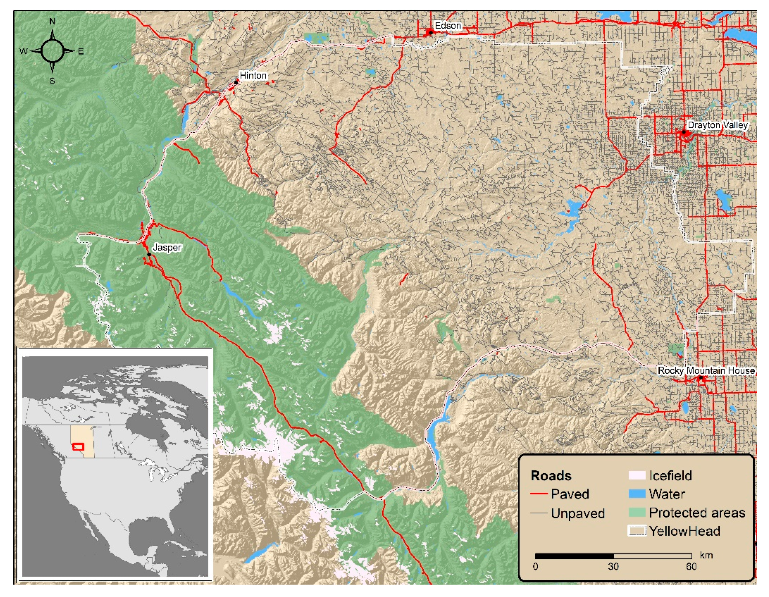
2.1. Study Area

This study focused on unpaved roads within the Yellowhead Bear Management Area (BMA 3), covering approximately 28,774 km² in west-central Alberta, Canada for an interior population of grizzly bears. The area follows a distinct east–west gradient with the western extents comprised of alpine and sub-alpine sections of the Canadian Rocky Mountains, whereas central and eastern sections are comprised of montane forest as well as upper and lower foothills [33]. The central and eastern portions outside of Jasper National Park are highly fragmented by unpaved road networks constructed for oil and gas exploration, agriculture, timber harvesting, coal mining, and wildfire suppression (Figure 1). Recreational activities are varied and widespread throughout the region and include hiking, camping, hunting, biking and off-road motorsports (e.g., ATVs, motorcycles). Many of the unpaved roads have ‘unimproved’ surfaces and are built for short term resource extraction activities rather than permanent access, and recreation activities along these roads may be inhibited by gates, barriers, seasonal closures or complete road deactivation once industrial activities cease. Other unpaved roads built as throughways to towns or to access mines are more permanent with improved gravel surfaces, ongoing maintenance and uninhibited access.

2.2. Reference Classification

2.2.1. Provincial Road Data

The Government of Alberta maintains an authoritative and publicly available database of roads classified into 15 categories—five paved categories and 10 unpaved categories. We downloaded the road network encompassing the entire study area (Figure 1) from the GeoDiscover Alberta data portal in April 2018. About 13,800 km of unpaved roads existed within the study area, making up 85% of all roads. The road network data was split into individual segments at each road junction or intersection. These segments became the unit of classification for all three classification approaches.

2.2.2. Classification Method

For the reference classification, we grouped the ten unpaved road categories into a three-class ranking based on the authors’ knowledge of the area and the provincial road database, to be compared with the network- and image-based classifications. We ranked “two-lane gravel roads” as high use, “one-lane gravel roads” as medium use, and all other unpaved road classes (“unimproved”, “truck-trail”, “temporary”, “unclassified”, “road”, “winter-road”, “ford-winter-xing”, “ferry-route”) as low use. The two- and one-lane gravel roads tend to be permanent access routes while the other classes tend to represent temporary or unmaintained roads. Two-lane roads generally connect population centres while one-lane roads serve as ancillary branches to access the temporary or unmaintained roads, which are typically constructed for forestry activities and are often abandoned or decommissioned after logging is complete.

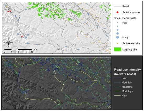
2.3. Network-Based Classification

2.3.1. Human Activity Data

For use in the network-based classification, we derived locations of human activity representing three types: (1) general activities (e.g., recreation and commerce); (2) oil and gas exploration and development; and (3) forest harvesting. The latter two represent the main natural resource extraction activities that occur in the region. We located general activities from posts to multiple social media platforms, specifically: Flickr, Facebook, Google and Wikilocs. We chose to combine platforms in order to capture a larger number of users, and account for the possibility of different usage patterns and activity types for different platforms [26].

In addition to locations of activity, we also quantified the intensity of activity at each location as follows. For Flickr data, we used their application programming interface (API) to extract photos for every centre-point in a 0.005-degree grid over the study area and counted the number of unique users that had posted photos within 500 m of each point. For Facebook data, we used their API to search for every named location within the study area and extracted the coordinates and the number of ‘check-ins’ for each location. For Google data, we used their API to locate every named place in the study area and then programmed a web browser to extract the number of reviews for each named place. For Wikilocs, a website of user-shared trails locations and information, we manually downloaded each available GPS track in the study area, extracted the start location of the track and the number of times the track had been downloaded. Initial locations and intensity values for each social media platform are shown in Supplementary Materials: Figure S1.

We filtered all locations to select those within 1 km of an unpaved road and ‘snapped’ the remaining locations to the nearest unpaved road. Therefore, posts within 1 km of each other were combined into a single location with a summed intensity value. We scaled the intensity values to the maximum of the study area for each respective social media platform, and combined posts from the four platforms into a single overall intensity value (Figure 2a). This was done to account for the fact that we did not restrict the time frame of location or intensity data, but rather included all data available on the date that data extraction occurred (approximately December 2018). The data, therefore, represent the cumulative activity across the landscape from when social media use became widespread (roughly 2005~2010) through approximately 2018. By combining datasets only after scaling each dataset separately, we sought to account for the fact that some platforms have been around longer than others and had different numbers of locations with data (Supplementary Materials: Table S1).

To identify locations of oil and gas activity, we extracted active well sites from the Alberta Biodiversity Monitoring Institute’s 2016 Human Footprint database [34] (Figure 2b). For locations of recent forest logging, we used satellite-detections of forest harvesting that occurred between 2014 and 2016 from the Landsat-derived forest change detection product originally developed in 2015 by [35] and updated in 2018 (Figure 2c).

2.3.2. Classification Method

We used “circuit theory” to develop a road classification approach based on the connection between known locations of human activity along the road network. Circuit theory is a connectivity model based on the movement of electricity through a connected network and has been applied across a variety of fields [36]. The circuit is simply a network of nodes connected by resistors. In our case, the nodes are locations of human activity and the resistors are the road network. When voltage is applied across a resistor (i.e., road) connecting two nodes (i.e., activity locations), the amount of current that flows between the two nodes is a function of the voltage applied, the resistance between the two nodes and the configuration of resistors between them. We used an open source software called ‘Circuitscape’ to apply circuit theory using spatial raster grids [37]. Specifically, we used Circuitscape version 4.0, programmed in Julia [38], which enabled processing at 5 m spatial resolution [39]. For a more detailed description of how circuit theory is applied to spatial raster grids, we refer readers to [36,37].

For each of the three types of activity, we iteratively applied voltage between each activity source and each of the activity locations (i.e., nodes; Figure 2). For general activities derived from social media posts, we defined sources as any post with an intensity >10th percentile that also overlaid nighttime lights visible in satellite imagery captured by the Defense Meteorological Satellite Program/Operational Linescan System (DMSP/OLS) (Figure 2a and Supplementary Materials: Figure S1e). For oil and gas and logging activities, we defined sources as the two largest population centers in the study area, which are where most workers live and where the two main sawmills are located (Figure 2b,c).

Input voltage was always held constant and a mask was applied to the study area such that the road network had a constant resistance of 1.0 and all grid cells outside the road network had infinite resistance (value of 0), which effectively allowed current to only flow along the road network. This meant that the initial current output of the Circuitscape algorithm was based solely on the spatial configuration of the activity sources, the activity locations and the road network. However, in the case of the current derived from the social media locations, the current output was then weighted by multiplying the current by the intensity value of the activity location used for each iteration. We summed the currents produced for each activity type and extracted this value for each road segment (Supplementary Materials: Figure S2). We then split the road segments into three categories using the summed current values, still for each activity type, based on percentiles of all observed summed values within each activity type as follows: low ≤ 10th percentile > medium < 90th percentile ≥ high. Finally, we combined the three activities into a single ranking: if two or more of the individual activity rankings were low, the overall ranking was low use; if two or more were high, the overall ranking was high use; otherwise, the overall ranking was medium use.

2.4. Image-Based Classification

2.4.1. App-Based Road Data

We collected data on road surface conditions and travel speed for a subset of the study area using a free mobile app called RoadLab-Pro, originally developed by the World Bank (see progressana.com accessed on 28 June 2021). When activated, the app uses the GPS receiver in a mobile device to automatically track location and travel speed and uses the device’s accelerometer to estimate road surface roughness. Six different users working for industrial and non-profit organizations operating in the region agreed to collect data for this project during daily work routines between June 2018 and March 2019 (e.g., checking oil and gas well sites, conducting wildlife surveys, etc.). Data coverage totalled approximately 1000 km of roads and 771 unique road segments, which we used as training data for the image-based classification.

2.4.2. Satellite Data

For use in the image-based classification, we obtained orthorectified (Level 3A) RapidEye satellite imagery acquired between 8 August and 17 September 2017. The RapidEye constellation of commercial satellites produces moderately high-resolution images (5 m pixels) with the capability of frequent imaging (revisit time of 1.0–5.5 days) over large areas [40], which is a useful platform for road monitoring in rural areas [21]. RapidEye imagery provides five bands covering the visible blue (440–510 nm), green (520–590 nm) and red (630–685 nm) wavelengths, as well as a red-edge band (690–730 nm) and a near-infrared band (NIR; 760–850 nm) that are each highly sensitive to green vegetation.

We mosaicked the RapidEye imagery into a single multi-band image, thus representing conditions during late summer 2017. From the multi-band RapidEye imagery, we generated a suite of seven vegetation indices (

Table 1. Vegetation indices from RapidEye imagery and terrain metrics used for feature extraction as inputs to the random forest model for the Image-based classification.

Variable	Description	Formula
Vegetation indices
NDVI	Normalized Difference Vegetation Index	$\frac{NIR-Red}{NIR+Red}$
NGRDI	Normalized Green-Red Difference Index	$\frac{Green-red}{Green+Red}$
RECI	Red-Edge Chlorophyll Index	$\frac{NIR-Red}{\left(NIR+Red\right)-RedEdge}$
RENDVI	Red-Edge Normalized Difference Vegetation Index	$\frac{NIR-RedEdge}{NIR+RedEdge}$
RG-ratio	Red/Green Ratio	$\frac{Red}{Green}$
SUM	Sum of visible bands	$Blue+Red+Green$
BARESOIL	Bare Soil Index	$\frac{Red+Blue-Green}{Red+Blue+Green}$
Terrain variables
DEM	Elevation (m)
INSOL	Insolation
SLOPE	Slope (degrees)
TWI	Topographic Wetness Index	$TWI=ln\left(\frac{f}{\tan s}\right)$ *

* where, f = upslope contributing area; and s = slope.

) related to vegetation cover and soil composition in forested environments [41,42], with the expectation that variation in vegetation and soil reflectance would be associated with road surface conditions and margins that, in turn, are associated with use intensity. For example, heavily used roads are required to be constructed with gravel and have wider margins cleared of tall vegetation. Lightly used or temporary roads are more likely to be unimproved tracks cut into the soil with narrower margins and vegetation regrowth on or along the road surface. We also generated four terrain variables from a 30 m digital elevation model produced from the National Aeronautics and Space Administration (NASA) Shuttle Radar Topography Mission (SRTM) (Table 1). In addition to the simple terrain variables of elevation and slope, we included insolation (a measure of primary energy received from the sun accounting for variation in elevation and aspect; calculated in ArcMap 10.6) and a topographic wetness index (a measure of near- and at-surface water accumulation) under the assumption that these represent patterns of snow melt and soil conditions which in turn influence where different types of road are constructed. For example, primary roads may be less likely to traverse a steep north slope which will hold snow and may become impassable in winter. We calculated descriptive statistic metrics for the seven vegetation indices and four terrain variables for a 25 m buffer around each road segment using Feature Extraction 2.7 (FETEX) software [43] (Supplementary Materials: Table S2). The 25 m buffer was used to account for roads of differing widths, road margins, and spatial errors that may exist in the GPS-derived road vector data and orthorectified satellite imagery. The FETEX 2.7 software was developed to characterize and classify agricultural parcels, but is applicable to any vector overlay and provides a computationally efficient means to extract a variety of spatial metrics. In addition to the descriptive statistics from the vegetation indices and terrain variables, we also used FETEX 2.7 to compute textural and semi-variogram metrics (Supplementary Materials: Table S2) from the NIR band, which is sensitive to green vegetation. Within the FETEX program, we set the parcel perimeter buffer to 2 pixels and did not specify a minimum parcel size. For the texture metrics extraction, we set the grey-level co-occurrence matrix (GLCM) grey levels at 64 and for the semi-variogram metrics extraction we set the lag size to 20 pixels and the random pixels percentage to 15. All other settings were left as defaults see [43]. Semi-variogram metrics detail the spatial patterns of pixel values, and are useful when performing classification from high resolution imagery in forested landscapes [44,45]. We expected that these metrics would be helpful to distinguish wider roads with homogenous surfaces and margins (i.e., lower roughness, higher speeds) from narrower roads with variable surfaces that may be occluded by overstory vegetation (i.e., higher roughness, lower speeds).

2.4.3. Classification Method

Using training data collected from RoadLab Pro and the FETEX metrics derived from RapidEye imagery as predictors, we classified speed and roughness of road segments using supervised random forest classifications programmed with the caret package in R [46]. Prior to modelling, continuous speed and roughness training data were grouped into three discrete classes (low, medium, and high) based on visual inspections of histograms of the distribution of each variable. The three speed classes were separated at 40 and 65 kph (Supplementary Materials: Figure S3) and the roughness classes at 2.2 and 3.4 (unitless index values; Supplementary Materials: Figure S4). Predictions were made for all road segments longer than 250 m. For segments shorter than 250 m, we assigned the majority predicted value of the longest segment they adjoined. The final three-class road classification of low use, medium use and high use combined the speed and roughness classifications by first ranking each separate prediction from 1–3 (low to high), then summing the two rankings, and finally re-ranking the summed values as low use = 2–3, medium use = 4, and high use = 5–6.

Prior to classification, Pearson’s correlation coefficient (r) was used to assess multi-collinearity of all spectral predictors. A single metric from groups of highly correlated variables (r > 0.8) were included as predictors in classifications, resulting in a total of 38 possible predictors remaining from the initial 106 candidate predictors. In order to reduce data dimensionality all predictor metrics were standardized to have a mean of 0 and standard deviation of 1 [47,48]. All models were generated using 10-fold cross-validation and were assessed based on the overall accuracy using the out-of-bag error estimate [49].

2.5. Statistical Analysis

2.5.1. Road Classification

We first compared the classification agreement between the network-based, image-based and reference approaches. Since classification was performed at the level of individual road segments, but segments can differ in length, we calculated the classification agreement as a function of road length (i.e., the total km of road segments with class agreement or disagreement between approaches).

2.5.2. Grizzly Bear Response to Roads

We obtained GPS locations for 56 grizzly bears collected between March and October from 2014 to 2017, resulting in a total of 83 unique “bear-years” (i.e., an individual bear observed in a given year; bears observed for multiple years were considered as multiple bear-years). Grizzly bears were captured and collared by biologists from the fRI Research Grizzly Bear Program (Hinton, Alberta) as part of long-term research and to inform provincial recovery efforts. Individuals were fit with Followit Iridium satellite collars programmed to collect locations every 30 min or hourly. All animal capture and handling followed the Canadian Council of Animal Care Guidelines and were permitted annually through the University of Saskatchewan Animal Care Committee. See [50] for detailed information about grizzly bear capture and handling.

We evaluated population level movements and habitat selection of grizzly bears relative to non-classified roads (“Any road”) and roads classified using the three methods described above. More specifically, we compared how movement rate changed and habitat selection varied by time of day—nocturnally and diurnally—for each road class as a function of distance to road. We predicted that grizzly bears would alter their behaviour when using areas within ~1000 m of high-use roads by increasing nocturnal activity due to some perceived risk attributed to human activity levels. If grizzly bears were responding to high-use roads in this manner, we expected movement rates would change and selection would be stronger at night [17].

For each bear-year, when 10 or more consecutive GPS relocations were available, we calculated the movement rate (m/hR) and turning angle between each relocation (i.e., step) using the amt package in R [50]. To analyze changes in typical movement patterns near roads of different classes, we first modeled movement rate across all relocations using a generalized additive model (GAM). Grizzly bear movement tended to follow a diurnal pattern, with reduced activity at night and increased movement during the day, especially in the morning and evening [51], and some variation between age-sex-reproductive classes (Figure 3). Movement also tended to be greater when the turning angle between steps was low, i.e., when grizzly bears are moving more linearly (Figure 3). Based on these observed trends, we modeled movement rate as a function of age-sex-reproductive class, hour of the day and turning angle. We smoothed hour of the day using a cyclic cubic regression spline and included an interaction with age-sex-reproductive class. We cosine-transformed turning angle and used a cubic regression spline for smoothing.

Once this model was created, we analyzed deviations from expected movement rates (i.e., model residuals) within 1000 km of unpaved roads in general (i.e., “Any road’”), and for each class within each of the three road-use classifications approaches. We were particularly interested in how deviations differed during the day and at night to determine if grizzly bears appeared to be more nocturnal around high-use roads.

We also analyzed habitat selection of grizzly bears at the level of the home range (third-order) by generating 100% minimum convex polygons (MCPs) for each bear and year. Because we were interested in grizzly bears’ response to unpaved roads, we clipped out areas of the home range where paved roads were closer than unpaved roads. We then created separate datasets for those GPS locations that occurred during day-time hours, which included twilight, versus those that occurred during night based on sunrise, sunset, and civil twilight tables [52]. For each dataset and use location, we generated 10 random ‘available’ locations within each MCP and extracted the distance to the nearest road of each of the three classes and for each classification approach. We then transformed each distance variable using an exponential decay of the form 1-(e^-αd) where d was the distance in meters and α was set to either 0.02 (fine scale, within ~200 m) or 0.002 (large scale, within ~2000 m). In doing so, the effects of roads would be localized to within meters (fine scale) or hundreds of meters (large scale). To ensure that our sample population of grizzly bears had each road type available, we calculated for each animal the proportion of available locations where the nearest road was classified as low, medium, or high. We then removed those individuals that did not have all three road classes available or where availability was less than 5%.

We used generalized linear mixed-effects models (GLMM) to estimate population-level RSF model coefficients with the lme4 package in R version 3.6.2 [53,54]. To ensure independence of our sample population and account for unbalanced sample sizes, we specified animal ID as a random intercept for all models [55]. For each dataset (i.e., day and night) and scale, we fit (1) a null (intercept-only) model, (2) a model that included distance to road without classification as a fixed effect, and (3) a model that also included a random slope and intercept for distance to road by road classification type. We used Akaike information criteria (AIC) scores to identify the model that best fit the data, with the best fitting model identified as that having the lowest AIC score and was not within two AIC units of a model with fewer parameters [56].

3. Results

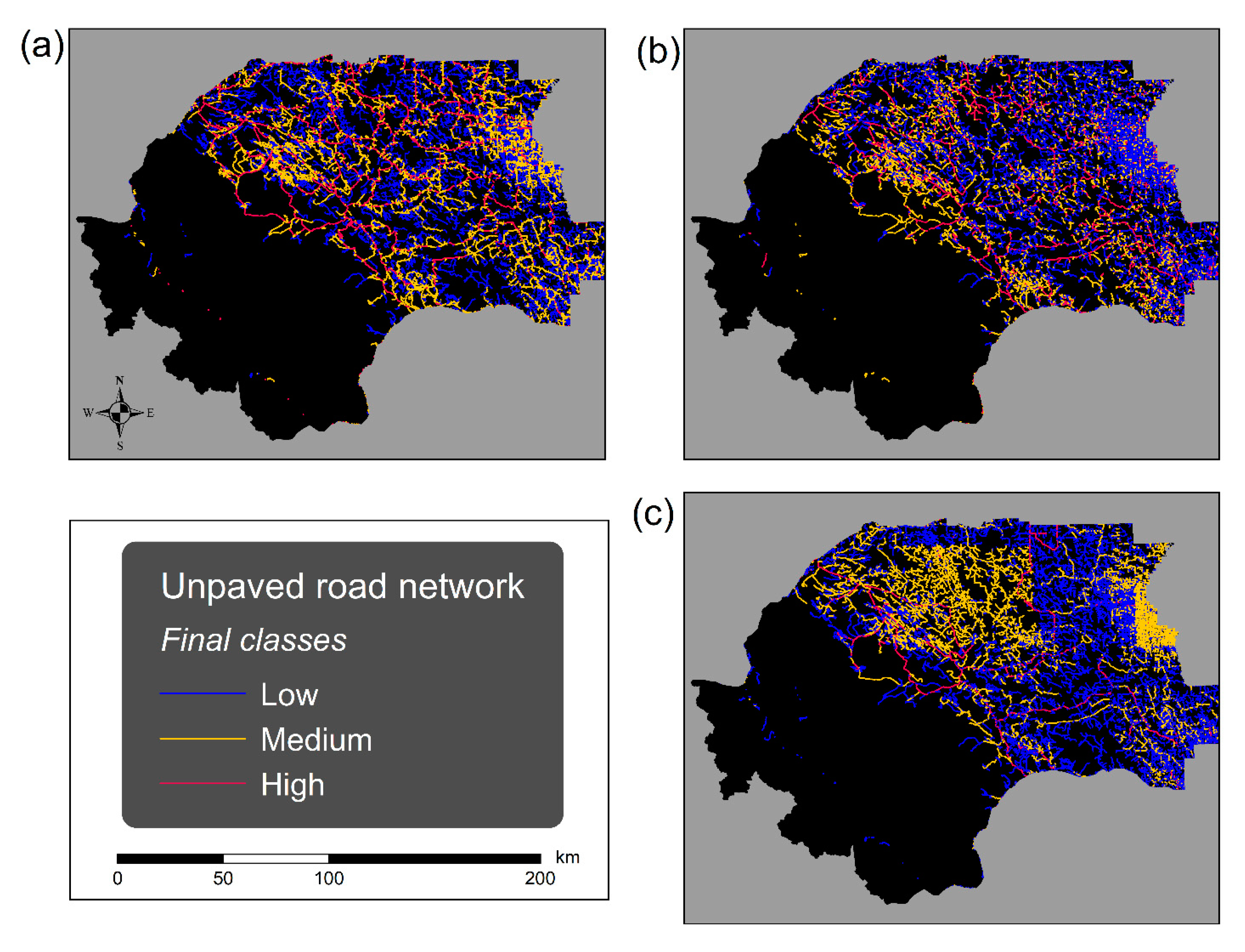
3.1. Road Classification

Overall accuracies for speed and roughness were 66% and 55%, respectively (

Table 2. Confusion matrix for predicting roughness and speed for individual road segments (n = 771) using RapidEye satellite imagery trained with data collected with the RoadLab-Pro app. Values are the total km of road segments classified into each category.

Roughness					Speed
	Observed			User’s Accuracy		Observed			User’s Accuracy
Predicted	Low	Med	High		Predicted	Low	Med	High
Low	127.7	57.7	15.9	63%	Low	23.3	23.0	5.0	45%
Med	108.7	286.1	135.4	54%	Med	89.5	389.6	118.2	65%
High	8.6	38.3	38.2	45%	High	0.0	44.4	122.9	73%
Producer’s Accuracy	52%	75%	71%	55%	Producer’s Accuracy	21%	85%	48%	66%

). For both speed and roughness, the semi-variogram metrics were the most important in the models, comprising five of the ten most important variables for each (Supplementary Materials: Figures S5 and S6). The vegetation indices tended to be more important than the terrain metrics. The most frequently high-ranking vegetation indices were BARESOIL (Bare Soil Index) and RENDVI (Red-Edge Normalized Difference Vegetation Index). DEM (Elevation) was the only terrain metric appearing in the 10 most important variables.

Generally, all three classifications estimated the length of road in each ranking to be low > medium > high, however, the spatial patterns of road rankings differed between the classifications (

Table 3. Three-way confusion matrix showing class agreement between the network-based, image-based and reference road characterization approaches for the three classes low use, medium use and high use. Values are in km of road segments classified to each road use. Agreement is calculated as the percent of the total km of road segments for a given row or column that were classified the same between the two respective approaches.

Network- Based	Reference					Image-Based
	Low	Med	High	Total	Agreement	Low	Med	High	Total	Agreement
Low	4436	1849	10	6295	70%	4189	1710	396	6295	67%
Med	2582	2645	321	5548	48%	2687	1819	1043	5548	33%
High	387	1079	507	1973	55%	494	603	876	1973	31%
Total	7405	5573	838	13,816		7370	4132	2314	13,816
Agreement	60%	47%	60%		55%	57%	44%	38%		50%
Image- Based
Low	4934	2391	45	7370	67%
Med	1989	1960	182	4132	47%
High	482	1221	611	2314	53%
Total	7405	5573	838	13,816
Agreement	67%	35%	73%		54%

, Figure 4). Overall pairwise class agreement for the three classifications ranged from 50–55%. The reference classification resulted in fewer total km of roads classified as high use (838 km) compared to the network-based (1973 km) and the image-based (2314 km) classifications. There was poor class agreement for high use between the network- and image-based methods (<40%), and more of the road network that ranked as high in the reference classification was ranked as high in the Image-based classification (73%) compared to the network-based classification (60%). The majority of the other road segments ranked as high by the image- and network-based approaches were ranked as medium in the reference classification. The image-based classification had less medium use roads (4132 km) compared to the network-based and reference classifications (5548 km and 5572 km, respectively). Across all three classifications, there was more inter-classification between medium and low rankings compared to medium and high rankings, and it was rare (<5%) for a road segment to be low in one classification and high in another (Table 3).

3.2. Grizzly Bear Response To Roads

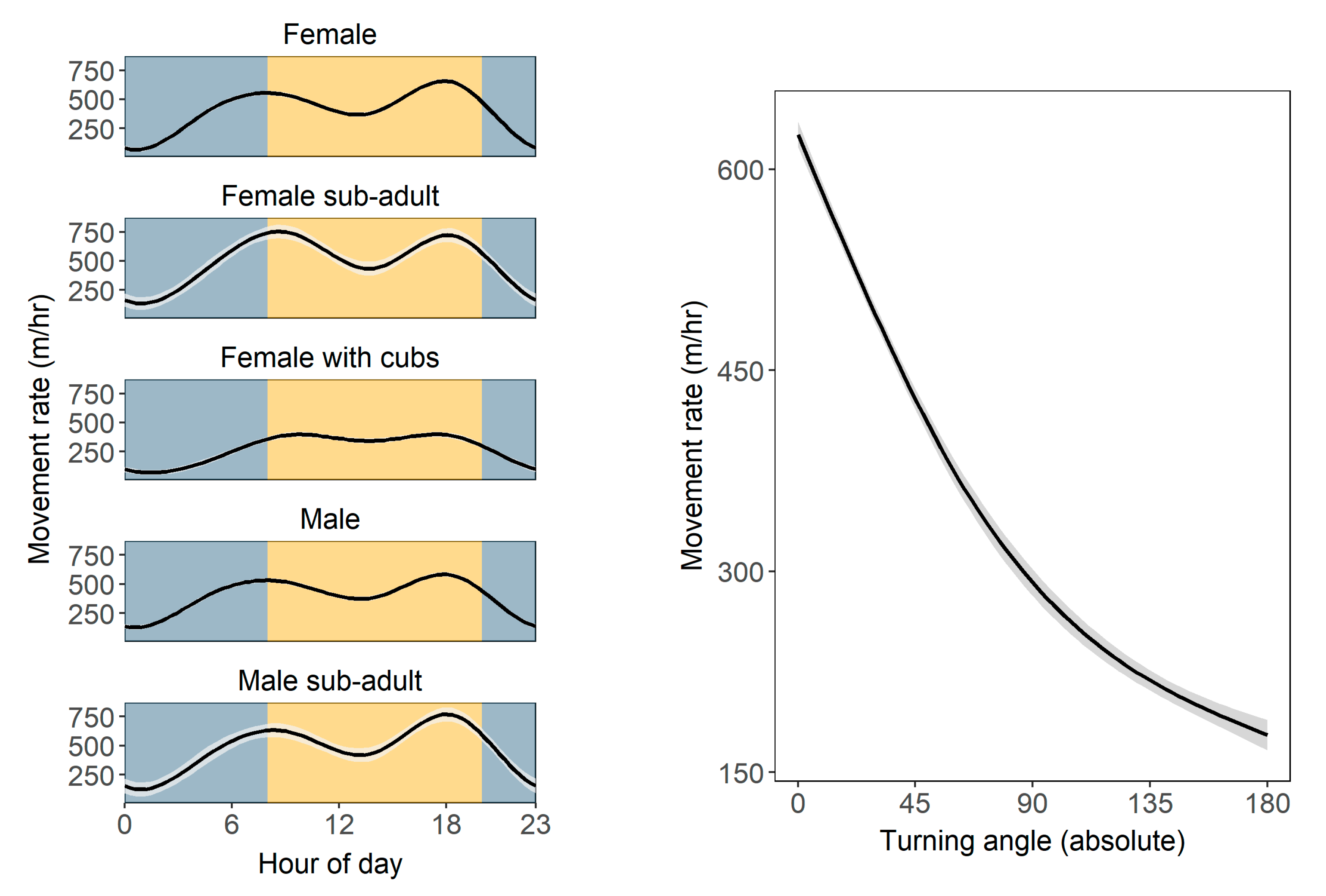
3.2.1. Grizzly Bear Movement

Analysis of grizzly bear movement rates within 1000 m of roads showed evidence of increased nocturnal activity. Compared to typical movement rates across the entire study area, when grizzly bears were within 1000 m of any unpaved road (i.e., not classified), movement was slightly greater than expected at night and slightly less than expected during the day (Figure 5). Within 1000 m of high use roads, the trend was more pronounced for all three classifications, and it was strongest for high use roads as classified by the image-based approach (Figure 5). In this case, the deviation from expected movement rates was 3–4 times higher compared to the medium- and low-use roads.

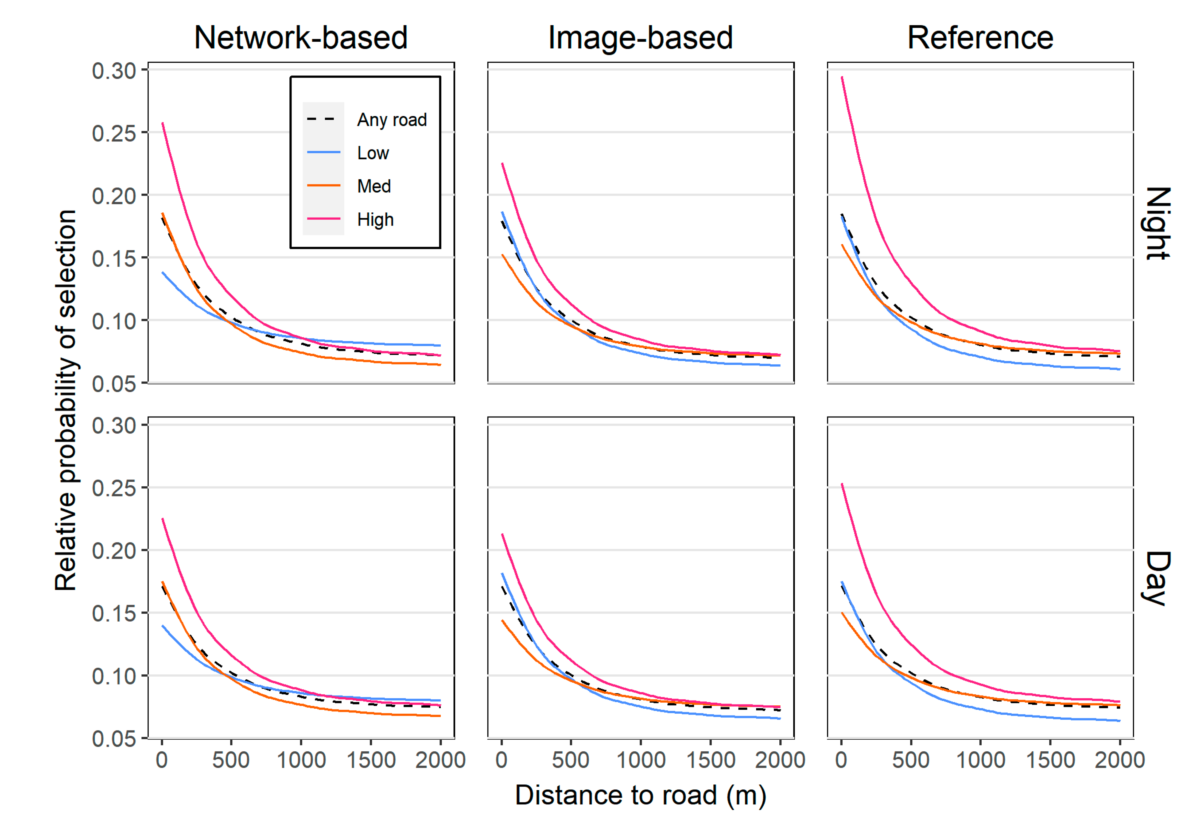
3.2.2. Grizzly Bear Selection

Our sample population to fit GLMM models consisted of 23 and 21 grizzly bears and 56,575 and 26,003 GPS relocations for the day and night datasets, respectively. Our preliminary evaluation indicated that irrespective of the specific road classification method, models fit better where road class was considered. Because of this, we used AIC to compare only the three classification methods for each dataset to identify the model that best fit the data (

Table 4. Comparison of generalized linear mixed-effects models describing the habitat selection of grizzly bears based on road classification method, time of day and scale using Akaike information criteria scores (AIC), where lower AIC scores indicates better model fit within a group. ΔAIC is the difference between the AIC score of that model and the lowest AIC score of the group. AIC_w is the AIC weight (0–1 possible), an indication of the probability that a given model is the best model of the group. Sample sizes: Night = 21 grizzly bears (23,003 “used” locations), Day = 23 grizzly bears (56,575 “used” locations).

Time of Day	Scale	Model	AIC	ΔAIC	AICw
Night	200 m	Network-based	521,640.7	142.0	0.00
		Image-based	521,704.5	78.2	0.00
		Reference	521,562.5	0.0	1.00
	2000 m	Network-based	514,291.2	1636.5	0.00
		Image-based	514,291.2	1190.8	0.00
		Reference	514,291.2	0.0	1.00
Day	200 m	Network-based	1,135,300	116.9	0.00
		Image-based	1,135,165	252.2	0.00
		Reference	1,135,048	0.0	1.00
	2000 m	Network-based	1,123,326	984.5	0.00
		Image-based	1,123,326	1610.4	0.00
		Reference	1,123,326	0.0	1.00

). We also compared the effects of model coefficients for all road classification methods and unclassified roads (Figure 6 and Figure S7).

Based on model AIC scores and weights (AIC_w), the reference classification method best fit the data (i.e., lowest AIC score) regardless of time of day and scale (Table 4). Between the network- and image-based classifications, the network-based method better fit the data during the day and the image-based better fit the data at night regardless of scale.

The relative probability of habitat selection was highest near high use roads for all three classification approaches at the 2000 m decay scale (Figure 6). For the reference and image-based classifications, selection was higher near low-use roads compared to medium-, whereas the opposite was true for the network-based approach. When roads were not classified, the probability of selection was similar to low-use roads classified by the reference and image-based methods, and the medium-use roads from the network-based method. All trends were generally similar, although less pronounced, at the 200 m scale (Supplementary Materials: Figure S7).

4. Discussion

We found that the three road classification methods had moderate class agreement and showed similar broad spatial patterns of road use. Despite some inconsistencies, all three methods improved grizzly bear habitat selection modelling compared to using unclassified roads. Additionally, grizzly bears showed similar selection and behavioural responses across the three methods: greater selection near high use roads irrespective of time of day, but a stronger shift in movement rate near high use roads between daytime (lower) versus nighttime (higher) compared to low and medium use roads.

4.1. Road Classification

While the reference is not a true ground-truth, it is encouraging that the network- and image-based approaches based on remote observation showed at least some consistency with the reference classes—more than half of the nearly 14,000 km of unpaved roads in the study area were characterized into the same class across the three methods (Table 3). The Government of Alberta has devoted immense resources to produce and maintain a provincial database covering a wide range of road types, and there are few places in the world with such detailed information on unpaved rural and resource roads. However, even when such detailed road data are available, they may not be maintained at a frequency to permit analysis of temporal changes, which may be critical to habitat monitoring (e.g., [21]). For example, data inconsistencies can arise when data are collected at different time periods or in different jurisdictions. The network- and image-based approaches developed in this study show promise as cost-effective methods to characterize road use for wildlife conservation applications, although more work is needed to better understand their relative strengths and weaknesses. The relatively consistent response of grizzly bears in our models using all three methods suggests that the road segments for which there was consistent classification agreement are influencing grizzly bear behaviour in this region and even imperfect characterization may be sufficient to improve wildlife modeling.

Within this study area, given the lack of traffic data associated with rural roads across the region, it is not possible to determine with certainty whether any of the classifications represent human road use better than the others. The fact that all three show some agreement and provide more information than treating all unpaved roads as equivalent (e.g., Figure 5, Table 4) suggests that each of the methods could be used or adapted to the data availability of a given application. Each classification approach comes with advantages and disadvantages. For example, the reference classification is a simple approach when existing road databases provide additional attribute information that can be used as a proxy for road use activity. This study suggests that, in this region, the reference classes are appropriate elements to include when building grizzly bear habitat models for management purposes, and future research in this region should explore how other species respond to the reference classes. We encourage future studies to test classification systems available for other regions from public or open source datasets.

When pre-existing road classes are not available, or data are found to be inadequate or outdated, the image-based approach is likely the most objective and easily replicable across regions since it relies on spectral information derived from satellites and ground data that can be collected using widely available technology. The fact that the spatial distribution of high-, medium-, and low-use roads predicted using this approach was similar to the other two approaches suggests that there is a relationship between spectral reflectance patterns of roads captured by satellite and broad patterns of human activity.

The accuracy of predicting surface roughness and travel speed using moderately-high resolution RapidEye imagery and the FETEX-derived spectral variables was relatively low (Table 2), although we note that accurate predictions of road roughness and travel speed were not primary objectives in this study. However, this shows that more work is needed to predict these individual road features. Deep learning algorithms of higher spatial resolution imagery, both of which are becoming increasingly accessible, would likely improve results. Currently, there are few examples of successful satellite-based monitoring of road conditions (e.g., [30]), and while this study shows promise, more work is needed to develop highly accurate predictions. The development of such predictions could enable cost-effective monitoring of changes in road use over time, as well as other applications for monitoring road conditions for the purpose of maintenance or emergency response planning. Our study suggests that capturing spatial spectral variability (e.g., FETEX-derived semi-variogram metrics) may be particularly useful for characterizing unpaved roads with remotely sensed imagery at this spatial scale. It is important to note that classifications developed for one region may not be applicable to another region due to differences in road surface materials, as well as differences in the relationships between travel speed, road roughness, spectral reflectance and human activity. Furthermore, additional research is needed to better understand the conditions under which spatial spectral variability is related to road use and conditions. For example, the relationship may not hold in desert conditions where roadside vegetation is sparse or non-existent, or in urban conditions where roadsides are highly variable and managed for objectives unrelated to road use.

The network-based approach provides a framework from which to build innovative methods to translate the vast amount of spatially explicit human activity information shared on social media and available in other public and open databases into meaningful information to improve our understanding of human-environment interaction. Our application of Circuitscape—an algorithm developed to predict habitat connectivity—is a novel approach to quantifying road network activity. The method is uniquely designed to capture pinch points in the road network and, when parametrized with data of known locations of human activity (i.e., social media data), may be especially useful for identifying high-use road segments.

While social media databases represent a massive and rapidly growing source of information on the nature and intensity of human activity, such datasets are not without their limitations and potential biases. Age, socio-economic condition and other geo-demographics likely influence patterns in social media use, which may differ across platforms [26,57,58]. People engaging in activities where location is sensitive (e.g., hunting, fishing) may be less likely to make geo-tagged posts, whereas photogenic events such as blooming flowers or wildlife sightings could lead to a disproportionate number of posts relative to visitors at specific locations [26]. The latter may help explain why less of the road network was classified as low use with the network-based approach compared to the image-based and reference methods. A biased under-classification of low-use roads may also explain the reversed pattern in relative habitat selection between low and medium use roads in the network-based approach compared to the other two methods.

Different data sources will likely capture different activities. We sought to combine data from multiple social media platforms, along with satellite data and public records, in order to account for a wide range of activities. However, combining data through scaling and classification requires subjective decisions to be made about the relative contribution of each dataset to overall human activity and what level of activity is considered “high” or “low”.

4.2. Grizzly Bear Response to Roads

Our results suggest that incorporating road classification into habitat models provides additional information to explain grizzly bear response to roads compared to treating all roads as equal. We observed different patterns of movement and habitat selection for roads with different predicted human activity levels. Grizzly bears appear to be more active near high use roads at night, as indicated by greater movement rates (Figure 5) and stronger selection (Figure 6) for all classification approaches. Indeed, a recent study of more than 2500 individuals showed that grizzly bears inhabiting human-dominated landscapes do not necessarily avoid areas with greater human activity, but rather shift toward more nocturnal behavioural patterns [59]. Our results support this conclusion and suggest that the deviation from typical diel movement observed in Figure 5 does not reflect avoidance of high use roads, but rather distinct behavioural patterns. For example, low movement rates during the day could be an indication of foraging behaviour, or more cautious movements near high use roads, and rapid movement at night may indicate that grizzly bears are using these as travel corridors during that time. The fact that the probability of selection is greatest near high use roads (Figure 6 and Supplementary Materials: Figure S7) suggests that foraging, rather than caution, may be driving the lower daytime movement rates observed near high use roads. This selection of high use roads contrasts with findings by [17] in southern Alberta, where they found grizzly bears avoided roads with high traffic volumes (>100 vehicles per day) during the day. It is possible that traffic volumes on roads classified as high use in our study are still lower than those in more populated southern Alberta, or that the human activity datasets in our study do not fully capture traffic patterns.

Nonetheless, it is concerning that grizzly bears may be especially attracted to high use roads for foraging. Studies in western Alberta and eastern British Columbia have shown that more than 85% of all human-caused grizzly bear mortalities occurred within about 100 m of a road (most were shot, not hit by vehicles) [5]. If high use roads are more strongly associated with grizzly bear space-use, this could increase the likelihood of negative human–bear interactions. It is possible that high use roads are more attractive to bears as a result of site selection, disturbance, or for both reasons. Roads with greater traffic require wider road margins, resulting in more disturbance and more light penetration, both which can lead to enhanced production of grizzly bear foods [11]. Roadkill of small mammals and ungulates, which can attract bears, may be more abundant along the high use roads in this study area. While these roads are expected to have the greatest travel speeds and traffic volumes of all unpaved roads in the area, speed and traffic are still moderate or low compared to highways and our study shows they do not elicit avoidance in grizzly bears. Such roads with moderate traffic volume, but insufficient to elicit avoidance, are expected to have the largest number of ungulate and small mammal carcasses due to these animals behavioural response to roads [60]. Larger and more frequently travelled roads may also be more likely to be constructed within already existing attractive habitat, for example in flatter terrain and along riparian corridors, which are preferred by grizzly bears [11,61]. By incorporating spatially explicit estimates of food resources (e.g., from satellite imagery and modeling) along with road classifications into analyses of grizzly bear movement, future studies may reveal whether thresholds of human activity and food resources at which grizzly bear behaviour changes exist. A better understanding of the timing and nature of potential co-occurrence of grizzly bears and people along roads would enhance the toolkit of land managers to set policies such as temporary and permanent road access closures [5], site selection and construction guidelines for new road development and public outreach and education.

Analysis at finer temporal scales would likely yield a more nuanced understanding of human activity along road networks and their influence on wildlife behaviour. In this study, we used GPS collar data for grizzly bear movements from 2014–2017, and sought to represent cumulative human activity for approximately this period (i.e., active oil and gas wells in 2016, forest logging from 2014–2016 and cumulative social media activity as of late 2017). While our analysis of grizzly bear behaviour tested the assumption that human activity varied between daytime and nighttime, it is also expected that human activity would vary seasonally and year-to-year. All the datasets used in this study could be analyzed for separate years, while most of the social media datasets could also be analyzed sub-annually since they contain timestamps. Analyzing oil and gas or logging activity at sub-annual temporal scales would be more challenging since data on the timing of activities that may drive more frequent traffic or large-truck traffic are not available, although separate analysis for each human activity by type may show different broad scale grizzly bear responses based on the type of traffic associated with each activity. Such analysis was beyond the scope of this study, which had the primary objective of describing and comparing the newly developed road characterization methods. However, it is important to note that analysis at finer temporal scales and by type of human activity may reveal different patterns of human activity and grizzly bear behaviour in this study area.

5. Conclusions

This study demonstrated that remotely sensed and crowd-sourced datasets can be used to estimate human use of unpaved roads within critical wildlife habitat to better understand the behaviour of threatened wildlife and quantify impacts. We found evidence of nocturnal behaviour by grizzly bears near high-use roads that was not evident when roads where unclassified. Perhaps most importantly, for grizzly bears in this study area, including any of the three classifications examined for this research improved the fit of movement and habitat selection models. This underscores the importance of characterizing road attributes related to indirect effects on wildlife (e.g., human activity), even for unpaved rural roads. When existing road databases include road attribute information (i.e., the reference in this study), this can be explored to develop proxies for the hypothesized indirect effects specific to a region. When such information is not available, the network-based and image-based classifications developed in this study provide examples of how emerging large datasets can be utilized for wildlife research and conservation where infrastructure development is widespread.

References

1. Benítez-López, A.; Alkemade, R.; Verweij, P.A. The impacts of roads and other infrastructure on mammal and bird populations: A meta-analysis. Biol. Conserv. 2010, 143, 1307–1316. [Google Scholar] [CrossRef] [Green Version]
2. Bennett, V.J.; Betts, M.G.; Smith, W.P. Toward Understanding the Ecological Impact of Transportation Corridors; U.S. Department of Agriculture, Forest Service, Pacific Northwest Research Station: Portland, OR, USA, 2011. [Google Scholar]
3. Boulanger, J.; Stenhouse, G.B. The impact of roads on the demography of grizzly bears in Alberta. PLoS ONE 2014, 9, e115535. [Google Scholar] [CrossRef] [PubMed] [Green Version]
4. Prokopenko, C.M.; Boyce, M.S.; Avgar, T. Characterizing wildlife behavioural responses to roads using integrated step selection analysis. J. Appl. Ecol. 2017, 54, 470–479. [Google Scholar] [CrossRef]
5. Proctor, M.F.; McLellan, B.N.; Stenhouse, G.B.; Mowat, G.; Lamb, C.T.; Boyce, M.S. Effects of roads and motorized human access on grizzly bear populations in British Columbia and Alberta, Canada. Ursus 2019, 2019, 16–39. [Google Scholar] [CrossRef] [Green Version]
6. Koen, E.L.; Bowman, J.; Sadowski, C.; Walpole, A.A. Landscape connectivity for wildlife: Development and validation of multispecies linkage maps. Methods Ecol. Evol. 2014, 5, 626–633. [Google Scholar] [CrossRef]
7. Proctor, M.F.; Paetkau, D.; McLellan, B.N.; Stenhouse, G.B.; Kendall, K.C.; Mace, R.D.; Kasworm, W.F.; Servheen, C.; Lausen, C.L.; Gibeau, M.L.; et al. Population fragmentation and inter-ecosystem movements of grizzly bears in Western Canada and the northern United States. Wildl. Monogr. 2012, 1–46. [Google Scholar] [CrossRef]
8. Moraes, A.M.; Ruiz-Miranda, C.R.; Galetti, P.M.; Niebuhr, B.B.; Alexandre, B.R.; Muylaert, R.L.; Grativol, A.D.; Ribeiro, J.W.; Ferreira, A.N.; Ribeiro, M.C. Landscape resistance influences effective dispersal of endangered golden lion tamarins within the Atlantic Forest. Biol. Conserv. 2018, 224, 178–187. [Google Scholar] [CrossRef] [Green Version]
9. Boulanger, J.; Cattet, M.; Nielsen, S.E.; Stenhouse, G.; Cranston, J. Use of multi-state models to explore relationships between changes in body condition, habitat and survival of grizzly bears Ursus Arctos horribilis. Wildl. Biol. 2013, 19, 274–288. [Google Scholar] [CrossRef] [Green Version]
10. Graham, K.; Boulanger, J.; Duval, J.; Stenhouse, G. Spatial and temporal use of roads by grizzly bears in west-central Alberta. Ursus 2010, 21, 43–56. [Google Scholar] [CrossRef]
11. Roever, C.L.; Boyce, M.S.; Stenhouse, G.B. Grizzly bears and forestry. I: Road vegetation and placement as an attractant to grizzly bears. For. Ecol. Manage. 2008, 256, 1253–1261. [Google Scholar] [CrossRef]
12. Mace, R.D.; Waller, J.S.; Manley, T.L.; Lyon, J.L.; Zuuring, H. Relationships among grizzly bears, roads and habitat in the Swan Mountains, Montana. J. Appl. Ecol. 1996, 33, 1395–1404. [Google Scholar] [CrossRef]
13. Benn, B.; Herrero, S. Grizzly bear mortality and human access in Banff and Yoho National Parks, 1971–98. Ursus 2002, 13, 213–221. [Google Scholar]
14. Nielsen, S.E.; Herrero, S.; Boyce, M.S.; Mace, R.D.; Benn, B.; Gibeau, M.L.; Jevons, S. Modelling the spatial distribution of human-caused grizzly bear mortalities in the Central Rockies ecosystem of Canada. Biol. Conserv. 2004, 120, 101–113. [Google Scholar] [CrossRef]
15. Nielsen, S.E.; Stenhouse, G.B.; Boyce, M.S. A habitat-based framework for grizzly bear conservation in Alberta. Biol. Conserv. 2006, 130, 217–229. [Google Scholar] [CrossRef]
16. Gibeau, M.L.; Herrero, S. Roads, rails and grizzly bears in the Bow River Valley, Alberta. In Proceedings of the State of Florida DOT Symposium, Fort Myers, FL, USA, 9–12 February 1998. [Google Scholar]
17. Northrup, J.M.; Pitt, J.; Muhly, T.B.; Stenhouse, G.B.; Musiani, M.; Boyce, M.S. Vehicle traffic shapes grizzly bear behaviour on a multiple-use landscape. J. Appl. Ecol. 2012, 49, 1159–1167. [Google Scholar] [CrossRef] [Green Version]
18. Hertel, A.G.; Swenson, J.E.; Bischof, R. A case for considering individual variation in diel activity patterns. Behav. Ecol. 2017, 28, 1524–1531. [Google Scholar] [CrossRef]
19. Kite, R.; Nelson, T.; Stenhouse, G.; Darimont, C. A movement-driven approach to quantifying grizzly bear (Ursus arctos) near-road movement patterns in west-central Alberta, Canada. Biol. Conserv. 2016, 195, 24–32. [Google Scholar] [CrossRef]
20. Scrafford, M.A.; Avgar, T.; Heeres, R.; Boyce, M.S. Roads elicit negative movement and habitat-selection responses by wolverines (Gulo gulo luscus). Behav. Ecol. 2018, 29, 534–542. [Google Scholar] [CrossRef]
21. Kearney, S.P.; Coops, N.C.; Sethi, S.; Stenhouse, G.B. Maintaining accurate, current, rural road network data: An extraction and updating routine using RapidEye, participatory GIS and deep learning. Int. J. Appl. Earth Obs. Geoinf. 2020, 87, 102031. [Google Scholar] [CrossRef]
22. Wang, W.; Yang, N.; Zhang, Y.; Wang, F.; Cao, T.; Eklund, P. A review of road extraction from remote sensing images. J. Traffic Transp. Eng. Engl. Ed. 2016, 3, 271–282. [Google Scholar] [CrossRef] [Green Version]
23. Yan, Y.; Kuo, C.L.; Feng, C.C.; Huang, W.; Fan, H.; Zipf, A. Coupling maximum entropy modeling with geotagged social media data to determine the geographic distribution of tourists. Int. J. Geogr. Inf. Sci. 2018, 32, 1699–1736. [Google Scholar] [CrossRef]
24. Wu, X.; Wood, S.A. Photos, tweets, and trails: Are social media proxies for urban trail use? J. Transp. Land Use 2017, 10, 789–804. [Google Scholar] [CrossRef] [Green Version]
25. Mancini, F.; Coghill, G.M.; Lusseau, D. Using social media to quantify spatial and temporal dynamics of nature-based recreational activities. PLoS ONE 2018, 13, e0200565. [Google Scholar] [CrossRef] [Green Version]
26. Tenkanen, H.; Di Minin, E.; Heikinheimo, V.; Hausmann, A.; Herbst, M.; Kajala, L.; Toivonen, T. Instagram, Flickr, or Twitter: Assessing the usability of social media data for visitor monitoring in protected areas. Sci. Rep. 2017, 7, 1–11. [Google Scholar] [CrossRef] [Green Version]
27. Wood, S.A.; Guerry, A.D.; Silver, J.M.; Lacayo, M. Using social media to quantify nature-based tourism and recreation. Sci. Rep. 2013, 3, 1–7. [Google Scholar] [CrossRef]
28. Vich, G.; Marquet, O.; Miralles-Guasch, C. Suburban commuting and activity spaces: Using smartphone tracking data to understand the spatial extent of travel behaviour. Geogr. J. 2017, 183, 426–439. [Google Scholar] [CrossRef]
29. Forslöf, L.; Jones, H. Roadroid: Continuous road condition monitoring with smart phones. J. Civ. Eng. Archit. 2015, 9, 485–496. [Google Scholar] [CrossRef] [Green Version]
30. Cadamuro, G.; Muhebwa, A.; Taneja, J. Assigning a grade: Accurate measurement of road quality using satellite imagery. ArXiv 2018, arXiv:abs/1812.01699. [Google Scholar]
31. Najjar, A.; Kaneko, S.; Miyanaga, Y. Combining satellite imagery and open data to map road safety. In Proceedings of the 31st AAAI Conference on Artificial Intelligence, AAAI, San Francisco, CA, USA, 4–9 February 2017; pp. 4524–4530. [Google Scholar]
32. Roever, C.L.; Boyce, M.S.; Stenhouse, G.B. Grizzly bears and forestry. II: Grizzly bear habitat selection and conflicts with road placement. For. Ecol. Manag. 2008, 256, 1262–1269. [Google Scholar] [CrossRef]
33. Achuff, P.L. Natural Regions, Subregions and Natural History Themes of Alberta: A Classification for Protected Areas Management—Updated and Revised; Alberta Environmental Protection, Parks Services: Edmonton, Alberta, 1994. [Google Scholar]
34. ABMI. ABMI Human Footprint Inventory: Wall-to-Wall Human Footprint Inventory; ABMI: Edmonton, AB, Canada, 2016. [Google Scholar]
35. Hermosilla, T.; Wulder, M.A.; White, J.C.; Coops, N.C.; Hobart, G.W. Regional detection, characterization, and attribution of annual forest change from 1984 to 2012 using Landsat-derived time-series metrics. Remote Sens. Environ. 2015, 170, 121–132. [Google Scholar] [CrossRef]
36. McRae, B.H.; Dickson, B.G.; Keitt, T.H.; Shah, V.B. Using circuit theory to model connectivity in ecology, evolution, and conservation. Ecology 2008, 89, 2712–2724. [Google Scholar] [CrossRef] [PubMed]
37. McRae, B.H.; Shah, V.B.; Mohapatra, T.K. Circuitscape 4 User Guide. The Nature Conservancy. 2013. Available online: http://www.circuitscape.org (accessed on 1 October 2019).
38. Bezanson, J.; Edelman, A.; Karpinski, S.; Shah, V.B. Julia: A fresh approach to numerical computing. SIAM Rev. 2017, 59, 65–98. [Google Scholar] [CrossRef] [Green Version]
39. Anantharaman, R.; Hall, K.; Shah, V.; Edelman, A. Circuitscape in Julia: High Performance Connectivity Modelling to Support Conservation Decisions. ArXiv 2019, arXiv:1906.03542. [Google Scholar]
40. Tyc, G.; Tulip, J.; Schulten, D.; Krischke, M.; Oxfort, M. The RapidEye mission design. Acta Astronaut. 2005, 56, 213–219. [Google Scholar] [CrossRef]
41. Hunt, E.R.; Doraiswamy, P.C.; McMurtrey, J.E.; Daughtry, C.S.T.; Perry, E.M.; Akhmedov, B. A visible band index for remote sensing leaf chlorophyll content at the Canopy scale. Int. J. Appl. Earth Obs. Geoinf. 2012, 21, 103–112. [Google Scholar] [CrossRef] [Green Version]
42. Abdollahnejad, A.; Panagiotidis, D.; Surový, P. Forest canopy density assessment using different approaches—Review. J. For. Sci. 2017, 63, 107–116. [Google Scholar] [CrossRef]
43. Ruiz, L.A.; Recio, J.A.; Fernández-Sarría, A.; Hermosilla, T. A feature extraction software tool for agricultural object-based image analysis. Comput. Electron. Agric. 2011, 76, 284–296. [Google Scholar] [CrossRef] [Green Version]
44. Goodbody, T.R.H.; Coops, N.C.; Hermosilla, T.; Tompalski, P.; McCartney, G.; MacLean, D.A. Digital aerial photogrammetry for assessing cumulative spruce budworm defoliation and enhancing forest inventories at a landscape-level. ISPRS J. Photogramm. Remote Sens. 2018, 142, 1–11. [Google Scholar] [CrossRef]
45. Goodbody, T.R.H.; Coops, N.C.; Hermosilla, T.; Tompalski, P.; Crawford, P. Assessing the status of forest regeneration using digital aerial photogrammetry and unmanned aerial systems. Int. J. Remote Sens. 2018, 39, 5246–5264. [Google Scholar] [CrossRef]
46. Kuhn, M.; Wing, J.; Weston, S.; Williams, A.; Keefer, C.; Engelhardt, A.; Cooper, T.; Mayer, Z.; Kenkel, B.; R Core Team; et al. Caret: Classification and Regression Training 2020. R Package Version 6.0-86. Available online: https://rdrr.io/cran/caret/ (accessed on 28 June 2021).
47. Strobl, C.; Boulesteix, A.L.; Zeileis, A.; Hothorn, T. Bias in random forest variable importance measures: Illustrations, sources and a solution. BMC Bioinform. 2007, 8. [Google Scholar] [CrossRef] [PubMed] [Green Version]
48. Van den Berg, R.A.; Hoefsloot, H.C.J.; Westerhuis, J.A.; Smilde, A.K.; van der Werf, M.J. Centering, scaling, and transformations: Improving the biological information content of metabolomics data. BMC Genom. 2006, 7, 1–15. [Google Scholar] [CrossRef] [Green Version]
49. Breiman, L. Bagging predictors. Mach. Learn. 1996, 24, 123–140. [Google Scholar] [CrossRef] [Green Version]
50. Cattet, M.; Boulanger, J.; Stenhouse, G.; Powell, R.A.; Reynolds-Hogland, M.J. An evaluation of long-term capture effects in ursids: Implications for wildlife welfare and research. J. Mammal. 2008, 89, 973–990. [Google Scholar] [CrossRef]
51. Signer, J.; Fieberg, J.; Avgar, T. Animal movement tools (amt): R package for managing tracking data and conducting habitat selection analyses. Ecol. Evol. 2019, 9, 880–890. [Google Scholar] [CrossRef] [PubMed]
52. Graham, K.; Stenhouse, G.B. Home range, movements and denning chronology of the grizzly bear (Ursus arctos) in west-central Alberta. Can. Field Nat. 2014, 128, 223–234. [Google Scholar] [CrossRef] [Green Version]
53. Munro, R.H.M.; Nielsen, S.E.; Price, M.H.; Stenhouse, G.B.; Boyce, M.S. Seasonal and diel patterns of grizzly bear diet and activity in west-central Alberta. J. Mammal. 2006, 87, 1112–1121. [Google Scholar] [CrossRef]
54. Bates, D.; Mächler, M.; Bolker, B.; Walker, S. Fitting linear mixed-effects models using lme4. J. Stat. Softw. 2015, 1. [Google Scholar] [CrossRef]
55. R Core Team. R: A Language and Environment for Statistical Computing; Version 3.6.0.; R Foundation for Statistical Computing: Vienna, Austria, 2019; Available online: https://www.R-project.org/ (accessed on 28 June 2021).
56. Gillies, C.S.; Hebblewhite, M.; Nielsen, S.E.; Krawchuk, M.A.; Aldridge, C.L.; Frair, J.L.; Saher, D.J.; Stevens, C.E.; Jerde, C.L. Application of random effects to the study of resource selection by animals. J. Anim. Ecol. 2006, 75, 887–898. [Google Scholar] [CrossRef]
57. Burnham, K.P.; Anderson, D.R. Model Selection and Multi-Model Inference: A Practical Information-Theoretic Approach, 2nd ed.; Springer Science & Business Media: New York, NY, USA, 2002; ISBN 978-0-387-22456-5. [Google Scholar]
58. Hausmann, A.; Toivonen, T.; Slotow, R.; Tenkanen, H.; Moilanen, A.; Heikinheimo, V.; Di Minin, E. Social media data can be used to understand tourists’ preferences for nature-based experiences in protected areas. Conserv. Lett. 2018, 11, 1–10. [Google Scholar] [CrossRef] [Green Version]
59. Hausmann, A.; Toivonen, T.; Heikinheimo, V.; Tenkanen, H.; Slotow, R.; Di Minin, E. Social media reveal that charismatic species are not the main attractor of ecotourists to sub-Saharan protected areas. Sci. Rep. 2017, 7, 1–9. [Google Scholar] [CrossRef] [Green Version]
60. Lamb, C.T.; Ford, A.T.; McLellan, B.N.; Proctor, M.F.; Mowat, G.; Ciarniello, L.; Nielsen, S.E.; Boutin, S. The ecology of human-carnivore coexistence. Proc. Natl. Acad. Sci. USA 2020, 117, 17876–17883. [Google Scholar] [CrossRef] [PubMed]
61. Jacobson, S.L.; Bliss-Ketchum, L.L.; De Rivera, C.E.; Smith, W.P. A behavior-based framework for assessing barrier effects to wildlife from vehicle traffic volume. Ecosphere 2016, 7, 1–15. [Google Scholar] [CrossRef]
Figure 1. Map of the road network within the study area in western Alberta, Canada.
Remotesensing 13 02547 g001
Figure 2. Maps of locations of the three types of human activity used in the network-based road-use classification: (a) recreation activity represented by social media posts, (b) oil and gas activity represented by active well sites and (c) recent forest logging activity detected by satellite. Activity sources represent where travelers to activity locations are likely to have originated. The activity sources and locations together represent the “nodes” used in the Circuitscape algorithm. Identification of activity sources is described in Section 2.3.1.
Remotesensing 13 02547 g002
Figure 3. Observed movement rate patterns across all grizzly bear locations by time of day for each age-sex-reproductive class (left) and by turning angle (right).
Remotesensing 13 02547 g003
Figure 4. Map the final classifications for all unpaved roads for (a) the network-based method, using circuit theory to connect activity locations for recreation, oil and gas extraction and logging; (b) the image-based method using RapidEye satellite imagery trained with road surface roughness and travel speed collected from a mobile app; and (c) the reference classification derived from the Government of Alberta provincial database, where classes were defined as: high = “o-lane gravel roads”; medium = “one-lane gravel roads”; low = and all other unpaved road classes (“unimproved”, “truck-trail”, “temporary”, “unclassified”, “road”, “winter-road”, “ford-winter-xing”, “ferry-route”).
Remotesensing 13 02547 g004
Figure 5. Fitted generalized additive models (GAM’s) of the deviation from expected grizzly bear movement rates (m/hr) by hour of the day for each road class within each of the three classification approaches, as well as for all unpaved roads (“Any road”; i.e., non-classified). Shading represents the 95% confidence interval.
Remotesensing 13 02547 g005
Figure 6. The relative probability of grizzly bear habitat selection as a function of road distance at the 2000 m scale by time of day (rows), classification method (columns) and whether roads were classified (colored lines; Low, Medium, or High human activity) or non-classified (dashed line; Any road).
Remotesensing 13 02547 g006