Article

Using Discrete-Point LiDAR to Classify Tree Species in the Riparian Pacific Northwest, USA

Huxley College of the Environment, Western Washington University, Bellingham, WA 98225, USA
*
Author to whom correspondence should be addressed.
Current address: School of Informatics, Computing, and Cyber Systems, Northern Arizona University, Flagstaff, AZ 86011, USA.
Remote Sens. 2021, 13(14), 2647; https://doi.org/10.3390/rs13142647
Submission received: 15 May 2021 / Revised: 11 June 2021 / Accepted: 2 July 2021 / Published: 6 July 2021
(This article belongs to the Section Forest Remote Sensing)

Abstract

:
Practical methods for tree species identification are important for both land management and scientific inquiry. LiDAR has been widely used for species mapping due to its ability to characterize 3D structure, but in structurally complex Pacific Northwest forests, additional research is needed. To address this need and to determine the feasibility of species modeling in such forests, we compared six approaches using five algorithms available in R’s lidR package and Trimble’s eCognition software to determine which approach most consistently identified individual trees across a heterogenous riparian landscape. We then classified segments into Douglas fir (Pseudotsuga menziesii), black cottonwood (Populus balsamifera ssp. trichocarpa), and red alder (Alnus rubra). Classification accuracies based on the best-performing segmentation method were 91%, 92%, and 84%, respectively. To our knowledge, this is the first study to investigate tree species modeling from LiDAR in a natural Pacific Northwest forest, and the first to model Pacific Northwest species at the landscape scale. Our results suggest that LiDAR alone may provide enough information on tree species to be useful to land managers in limited applications, even under structurally challenging conditions. With slight changes to the modeling approach, even higher accuracies may be possible.

Graphical Abstract

1. Introduction

Accurate mapping of the distribution of tree species is important both for scientific inquiry and for effective forest management [1,2,3,4]. Species-specific information can be used to refine stand-level estimates of growth, basal area, and other structural characteristics based on known allometric relationships [5,6]. Tree species identity is relevant to wildlife conservation and habitat mapping [7,8], can inform nutrient cycling models [9], and can influence decay rates and ecological functions performed by snags and woody debris [10,11,12]. Accurate species frequency maps are necessary when modeling potential changes to species distributions under future climate and disturbance scenarios [13], and in the long term, monitoring the distribution of species will be important for monitoring the realized effects of climate change [1,13].
Developing practical and accurate remote-sensing approaches to tree species classification remains an area of active research and development [3]. Many studies have focused on the use of light detection and ranging (LiDAR) for tree species classification because of its ability to detect 3D structures [2,14]. Often, the structural data from LiDAR are supplemented with multispectral imagery [3], but although this can improve model accuracies [15], it has the disadvantage of introducing an additional level of complexity to the model as well as being potentially more costly in terms of finance, time, worker skill, and computing resources. Among small-footprint aerial LiDAR systems (ALS) suitable for categorizing forests at the individual tree scale, both discrete-return and full-waveform data types exist. The full-waveform data provides more information than discrete-return data [4,14], but it is significantly more complex and not yet widely available to many project managers. In contrast, discrete-return ALS is much more widely available. In many parts of the United States, discrete-return LiDAR datasets have been collected by public entities and are now available for public download, making it an attractive and cost-effective option for researchers. Optimally, species models accurate enough for practical use could be derived from these publicly available datasets.
Tree species classification results and accuracies vary greatly based on the structure and composition of the forest [3,16]. For studies based on discrete-return ALS, accuracies of >90% were reported in multiple forest types [17,18,19,20,21,22], but accuracies can be much lower under less ideal conditions and depending on the target species and other factors [4,21,22]. In general, the first step in species modeling is to segment imagery or point clouds into smaller portions representing individual trees [4]. It is then possible to extract unique spectral or morphological features that allow the tree to be identified to species. However, the accuracy of this first crucial step is generally lower for trees that are shorter than their neighbors and trees in dense forests [23,24], and it has also been reported to be more challenging in deciduous-dominated forests [16]. Additional factors, such as the number of species present [4] and complexities related to terrain [25] or leaf-on/leaf-off conditions [4,22,26] can also affect species classification accuracies.
Riparian forests in the Pacific Northwest are more heterogeneous than their upland counterparts [27], which makes them a challenging subject to model. The structure of riparian Pacific Northwest forests varies greatly depending on the local geomorphology and the history of land use [28,29]. A single watershed may contain patches of large conifers, mixed deciduous forest, short dense “doghair” deciduous stands, and even planted stands of regularly spaced conifers, which may have uncharacteristic growth patterns relative to the same species in natural areas. Previous preliminary attempts to segment dense riparian Pacific Northwest forests into individual trees have not been very successful [30], although prior to now no formal assessment of multiple segmentation model performance had been carried out in this ecosystem. In addition to the segmentation and classification challenges resulting from varied stand density, channel movements tend to result in a gradient of tree ages [28], which precludes using height as a factor in species identification and complicates the identification of species-specific morphological traits. Such a landscape is very different from the study areas of most species classification studies [2], and it provides an excellent opportunity to study the strengths and weaknesses of species classification model approaches.
Hitherto, there has been relatively little research on distinguishing tree species in Pacific Northwest forests. The only studies to focus exclusively on LiDAR data were carried out in the Seattle Arboretum under intentionally simplified conditions [18,19,26]. These studies reported classification accuracies for discrete-point data ranging from 74.9% [26] to 97.8% [19] depending on the number of species being considered. In natural forests in British Columbia, Canada, another set of researchers used a fusion of 2D multispectral imagery and LiDAR data to classify tree species, resulting in user’s accuracies ranging from 63–87.8% for seven coniferous and broadleaf species [15].
The results from these previous studies suggest that discrete-point LiDAR, while not perfect, might still be capable of providing enough information on species composition to be useful to land managers. Therefore, the purpose of our study was to investigate the utility and practicality of species modeling under more complex forest conditions using readily available discrete-point LiDAR data. We focused on heterogonous riparian and river-adjacent hillslope forest in the Pacific Northwest because of its regional importance for salmon conservation [10,31], and we compared five different algorithms from two software packages to find the most accurate and practical method for tree segmentation and species modeling. Our goal was to evaluate existing methods of tree segmentation in this new environment and then determine the best possible accuracies for tree species classification, given the limitations of existing segmentation algorithms. Because we intended such workflows to be practical in a land management setting, we endeavored to keep the models as straightforward and with as few steps as possible while still allowing for reasonable accuracy in the results.

2. Materials and Methods
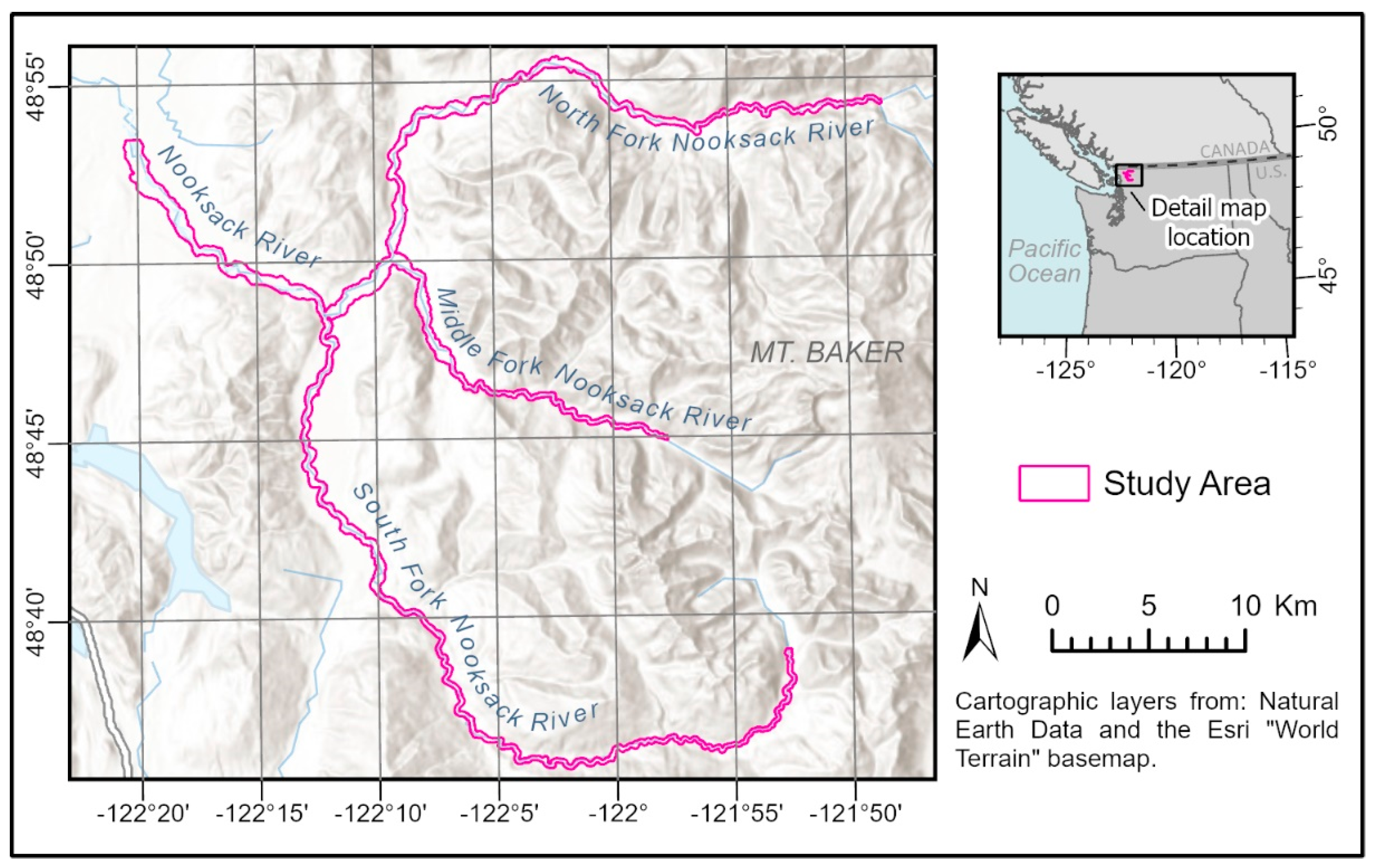
2.1. Study Area

The Nooksack River Watershed is located in northwestern Washington State, USA. The river is fed by the western slopes of the North Cascades. Steep slopes are common surrounding the confined upper reaches, whereas middle and lowland reaches flow through unconfined valleys at a lower gradient [32]. The upper reaches are primarily dominated by conifers, and the lower reaches are mostly dominated by deciduous stands of varying heights. The most common tree species present in the study area are red alder (alnus rubra), black cottonwood (Populus balsamifera ssp. trichocarpa), Douglas fir (Pseudotsuga menziesii), western hemlock (Tsuga heterophylla), bigleaf maple (Acer macrophyllum), and western redcedar (Thuja plicata). Other rarer species in the study area include paper birch (Betula papyrifera), cascara (Rhamnus purshiana), bitter cherry (Prunus emarginata), beaked hazelnut (Corylus cornuta var. californica), Sitka spruce (Picea sitchensis), vine maple (Acer circinatum), willows (Salix ssp.), and Pacific yew (Taxus brevifolia). The river has three forks that join and then flow into Bellingham Bay in Puget Sound, Washington [32].
Our study area consisted of the riparian zones of most of the three forks and a portion of the upper main stem (Figure 1). The boundary for the study area was defined by a 100 m buffer on the river’s recent migration zone, here defined as the area that had either been submerged for 50% or more of the time from 1933–2002 (as determined from aerial photographs, see Collins and Sheikh [33]) or that was designated active channel in the National Hydrography Dataset [34]. This definition was intended to facilitate remote mapping, minimize accidental inclusion of upland forests, and maximize the inclusion of true riparian stands. A 100 m buffer is wider than state- and federally mandated buffers and was intended to account for short-term channel migration.

2.2. LiDAR Data and Pre-Processing

The LiDAR dataset used for this project was collected in summer 2016 under leaf-on conditions by the United States Geological Survey (USGS). This was a multiple-return dataset with intensity data and an average point density of 8 returns/m2; for details, see Lowe et al. [35]. At the time of our study, this was the most up-to-date LiDAR data available for this region. The all-returns point cloud, a digital surface model, and a digital terrain model are publicly available through the Washington State Department of Natural Resources LiDAR Portal [36]. The intensity values in the point cloud were normalized using proprietary software by the vendor [35].
We used Fusion 3.8, a non-commercial LiDAR processing package developed by the US Forest Service [37] to create a series of rasters that represented over 30 different metrics derived from the LiDAR point cloud. The vendor-provided point cloud was normalized and filtered for outliers, then rasterized at 1-m and 30-m resolution using the Gridmetrics tool embedded in Fusion’s AreaProcessor [37]. The 30-m resolution rasters were intended for use in selecting locations to sample ground-truth data and were calculated from all returns above 3 m. The 1-m resolution rasters were intended for later use in the segmentation and species classification models and, based on model performance in preliminary trials, were calculated from only the first returns above 3 m. Various statistics calculated from these rasters at the individual tree level (for example, the mean value within the footprint of a single tree’s canopy) acted as the input variables for tree species classification (see Section 2.6). Rasters generated represented measures of height, variability in height, intensity, variability in intensity, canopy relief, canopy cover, and canopy structure (Table 1).

2.3. Ground-Truth Data Collection and Pre-Processing

Potential plot locations for ground-truth data collection were chosen using a proportional random sampling design. The objective was to collect data from at least 100 plots in the riparian zone at varying distances from the active channel. To select potential locations, we adapted methods described in the literature and used principal components analysis (PCA), k-means clustering, and GIS to determine how the primary factors influencing variability in the LiDAR data were spatially distributed [30,38,39]. With 15-m radius circular plots that were equivalent to the planned ground-truth plot dimensions, we used Esri’s ArcGIS to randomly sample 5900 non-water locations across the study area. These samples were clustered based on significant principal components calculated in R [40] for nine LiDAR metrics: maximum return height, mean return height, standard deviation of return height, 80th percentile of return height, canopy relief ratio, mean intensity, mode intensity, standard deviation of intensity, and percent cover. The characteristics of each cluster were then used to define a series of unique structural groups within the 2016 LiDAR data. Each structural group was mapped across the landscape, and then proportional random sampling was used to randomly place a corresponding number of plots within each structure type [41]. Potential plots were then evaluated using GIS for logistical constraints such as land ownership and accessibility. Most sites were also visited in person prior to sampling because the majority of randomly selected sites turned out to be inaccessible or unsafe. When this occurred, a nearby location in the same forest structural group was substituted. In the end, 37% of the plots were randomly placed, and the remaining 63% of all plot locations were chosen from locations near to the original randomized point ahead of time in the lab or (rarely) on the fly in the field.
All field data were collected between 1 July and 12 September 2019. Plots were circular with a 15 m radius (area = 707 m2 or 0.07 ha). This plot size was chosen to balance logistical practicality with minimizing edge effects, based on work by Frazer et al. [38], who found that plots ≥ 707 m2 produced substantially more accurate models than smaller size plots. We recorded height, diameter, coordinates relative to plot center (measured using a Leica TC600 Total Station and Trimble GeoXH Geoexplorer 6000 GPS) and various structural characteristics for all stems ≥ 10 cm in diameter and taller than 3 m (Table 2). We also recorded a brief description of the plot vegetation, gave a subjective assessment of the relative canopy closure, and noted terrain features such as steep slopes, marshy areas, or small streams running through the plot. Using the coordinates obtained using the total station, we sketched a rough tree-stem map for each plot. This helped us match height measurements to the correct trees and sped up data collection by making it easier to determine which trees were within the plot area.
Because not all plot locations were truly random, we used k-means cluster analyses in R [40] to confirm that randomly selected plots were not different from non-randomly selected plots (Appendix A). We also checked for spatial autocorrelation because it can, if present, affect which analyses are appropriate to use on a dataset. We used R to create directional variograms and calculate Moran’s I to assess potential spatial autocorrelation between plot-level variables [40,42,43].
Tree height was challenging to measure due to the prevalence of thick underbrush, unstable ground, and closed canopies in the study area. As a result, most plots contained several trees where either it was impractical to measure the height, or we could not definitively match canopy heights to the correct stems. When this occurred, we would note the heights of trees in the immediate area (inside or sometimes outside of the plot) that appeared representative for that species, dominance, and size class. Later, this supplemental height information was used to estimate values to fill in missing data prior to calculating overall plot metrics.
We created a series of height–diameter curves from the existing data by regressing tree diameter against tree height then using these species-specific relationships to predict heights from stem diameter. When supplemental height data were available for a given plot, they were used to refine the estimates given by the height–diameter curves. A value would be randomly selected from within the range of heights typical for that diameter and type of tree, then averaged with the predicted value given by the height/diameter curve. This weighted the final prediction towards site-specific conditions. This method was selected for its efficiency because each missing value had to be individually corrected. The resulting height data fell under the following four categories: (1) height was directly measured in the field, (2) height was estimated using height–diameter curves and was refined by field observations of typical tree heights within the plot, (3) height was estimated using height–diameter curves and was refined by field observations of tree heights from outside of the plot, and (4) height was estimated using height–diameter curves only. The processing method used for each height observation was documented and used to calculate the mode height method for each plot. To see if the estimated heights had introduced a detectable bias, we plotted the mean ground-truth height data against various LiDAR height metrics and looked for plot-level patterns or trends corresponding to the frequency and method of estimated height data in the plot.

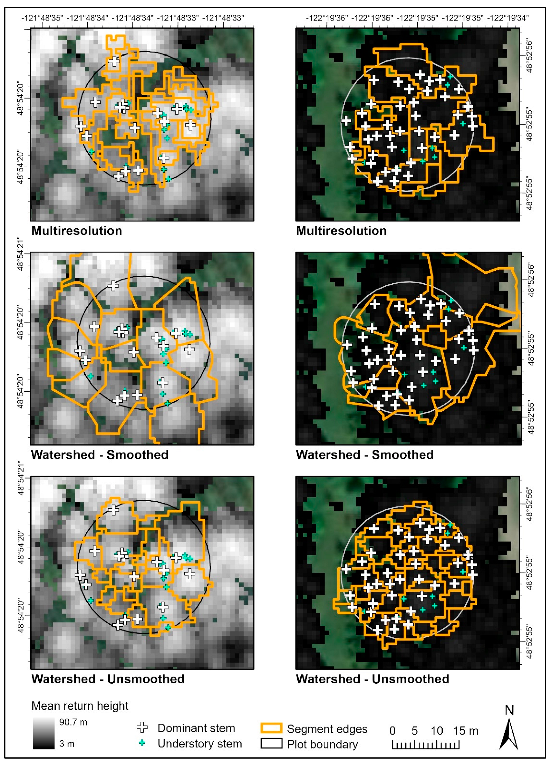
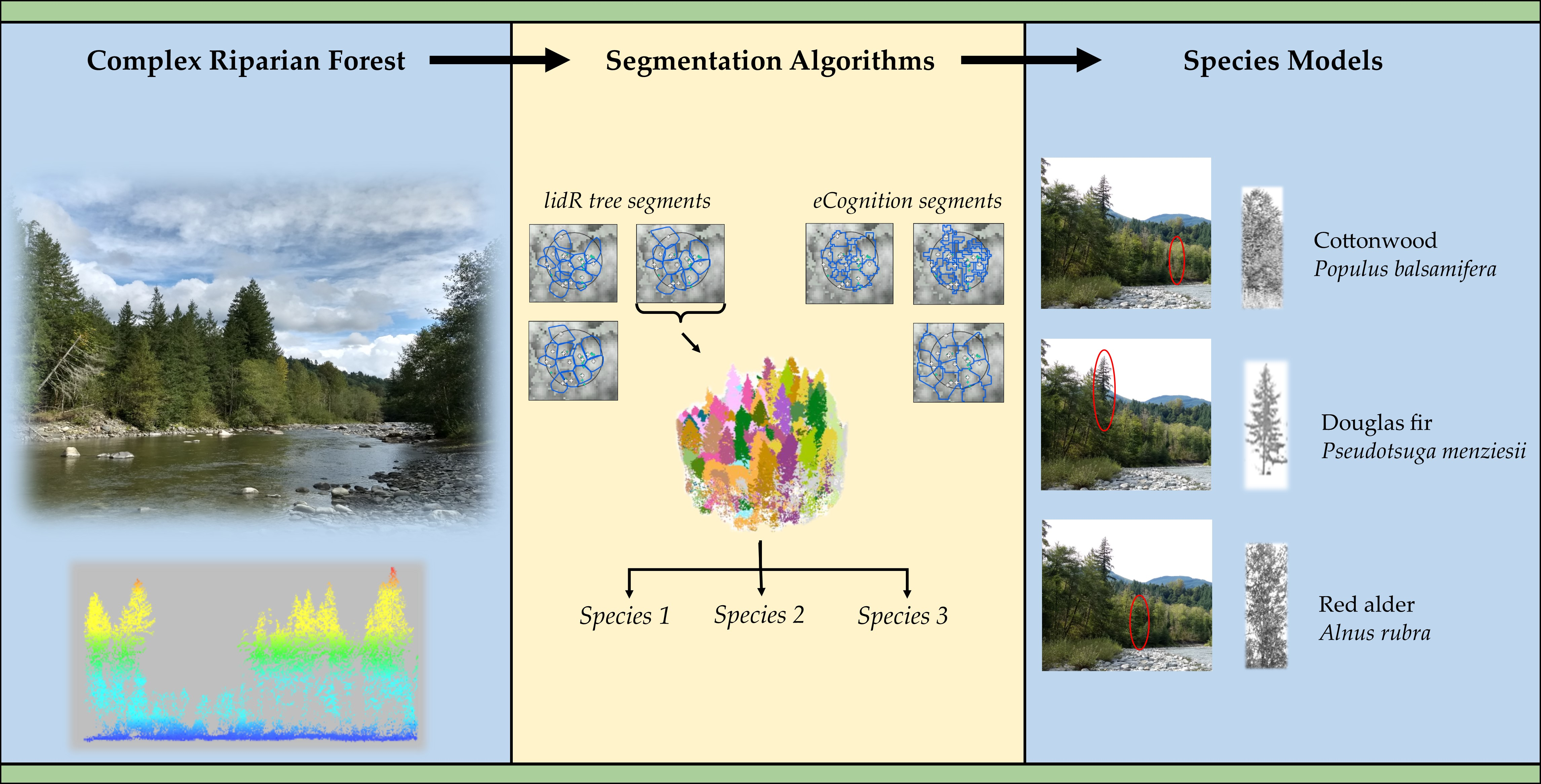
2.4. Individual Tree Segmentation

We compared six different approaches using five different algorithms for identifying individual tree canopies in the LiDAR data. Three of these approaches, (two versions of watershed segmentation and one version of multiresolution segmentation), were processed in Trimble’s eCognition Developer 9.5 [44] on the 1-m resolution rasters that were generated with Fusion’s AreaProcessor [37]. The remaining three approaches were processed entirely in the R programming environment [40] using the LiDAR processing package lidR [45]. In the lidR package, these three methods are called the “Dalponte2016”, “Silva2016”, and “Li2012” algorithms, and they implement methods developed by Dalponte and Coomes [46], Silva et al. [47], and Li et al. [48]. For consistency with the lidR package, we will refer to these three methods by their lidR function names.
Multiresolution segmentation in eCognition is an iterative algorithm that segments a raster by grouping pixels together until each segment reaches a variance threshold. Separate parameters control the algorithm’s sensitivity to brightness differences relative to the smoothness and compactness of the output segments. We used eCognition to run multiresolution segmentation on a 1-m canopy surface raster representing the mean height of LiDAR first returns. After using a 3-m height cutoff to remove non-forested areas from consideration, we processed all forested areas in the study area as a single unit under the same set of parameters. The scale, shape, and compactness parameters were set to 10, 0.1, and 0.5 respectively.
Watershed segmentation is a segmentation method that delineates image object boundaries from a canopy surface raster based on localized concavities and convexities in the data. The size and shape of output segments can be partially controlled by applying various smoothing filters to the input raster surface. We applied the eCognition watershed segmentation algorithm to two different rasters: an unsmoothed 1-m raster of the mean height of first returns, and a smoothed 1-m raster that we created from the 80th percentile of LiDAR first return heights, smoothed over a 3 × 3 window.
The Dalponte2016 algorithm in the lidR R package is a region-growing method developed by Dalponte and Coomes [46]. It requires a canopy surface model and a set of individual seed points representing treetops. We generated the input canopy surface model by applying lidR’s simple point to raster approach on the filtered, normalized point cloud [45]. We filled null values and smoothed the 0.6-m resolution surface across a 1-m window using the R package “raster” [49]. The parameters used in the Dalponte2016 segmentation were slightly modified from the defaults in order to make them more suitable for local conditions (Table 3).
We identified treetop locations in the LiDAR point cloud by using a local maximum filter to return the highest LiDAR return point in a given area [50]. The search window was defined using a multi-level function that allowed a different canopy radius for shorter trees than for large trees. We used a treetop detection function that assigned a circular search window diameter of 3 m to trees < 2 m tall, and a search window width of 5 m to trees > 20 m tall. Trees with heights between these cutoffs were assigned search window widths along a sliding scale. This balanced rates of accidental misclassification of tree branches as treetops with accurate detection of smaller inter-canopy trees. Additionally, LiDAR returns located less than 5 m off the ground were excluded from consideration as treetops because visual examination indicated that too many of these belonged to tall shrubs rather than trees. To facilitate a visual check of the model performance, we plotted the treetop results on top of subsets of the filtered and normalized point cloud.
The Silva2016 algorithm in lidR is a nearest-neighbor segmentation algorithm developed by Silva et al. [47]. Just as the Dalponte2016 algorithm, it uses a canopy surface model and treetop seed points. We used the same canopy surface and treetop points for both algorithms. This meant that both methods produced the same number of total segments per plot, though differences in segment size and shape could occur.
In contrast to the other two lidR algorithms, the Li2012 algorithm delineates trees directly from the point cloud without the use of the pre-determined treetops. The algorithm starts with the topmost LiDAR return point in the file, classifies all remaining points as either belonging to that tree or not based on variable distance criteria, then removes the classified points and starts over again with the next highest unclassified point, continuing until all points in the dataset are classified [45,46]. After trial and error, we used parameters that were very close to the default parameters recommended by Li et al. [48] (Table 3).
For all five methods, we assessed segmentation accuracy in terms of recall, precision, and F-score. The recall is the tree detection rate, precision is the correctness of detected trees, and F-score is an overall accuracy measure. We also assessed segmentation accuracy in terms of the correlation with ground-truth stem density, and we visually assessed how well the automatically generated segment shapes matched the shape and extent of the real tree canopy. Recall, precision, and F-score were calculated from the rates of true positives (TP), which represent correctly segmented trees, false positives (FP), which were segments that did not represent a ground-truth tree, and false negatives (FN), which were ground-truth trees that were not assigned their own segment. Recall, precision, and F-score were calculated as follows:
Recall = TP/(TP + FN),
Precision = TP/(TP + FP),
F-score = 2 × (recall × precision)/(recall + precision),
For the purposes of calculating segmentation accuracy metrics, we defined segments as “in” the plot if their centroid was located inside the plot. To avoid artificially inflated counts of true positives caused by overlapping segment boundaries (segments produced by lidR can overlap under certain conditions), the maximum number of true positives was not allowed to exceed the total number of dominant trees in a plot.

2.5. Individual Tree Metrics

We calculated individual tree metrics including height, diameter, and coniferous or deciduous classification for segments produced by the smoothed watershed method and by the Dalponte2016 algorithm. Because of their size, segments produced by the smoothed watershed method were analyzed with a localized area-based approach. If there was more than one dominant ground-truth tree in a segment derived from the smoothed watershed method, then the ground-truth data for the trees in that segment were averaged and the average ground-truth value was regressed against the average LiDAR-based value within that segment. (LiDAR-based values summarizing the attributes within the footprint of each individual tree segment were calculated from the 1-m resolution rasters generated from the first returns of the point cloud. See Section 2.2 for details). In contrast, the segments produced by the Dalponte2016 algorithm were analyzed using an individual tree approach, in which the segment LiDAR values were regressed against the individual ground-truth values of the largest dominant tree.
Because it was important to ensure that all segments were associated with complete ground-truth data, we used more stringent criteria for selecting in-plot segments for metrics generation than we had used for the segmentation accuracy metrics. Segments that we generated using the smoothed watershed method were paired with ground-truth data and counted as inside the plot if they were completely within a 2-m buffer around the plot and either the segment centroid was within the plot or the segment contained at least one dominant ground-truth stem.
Segments that we generated with the Dalponte2016 algorithm were paired with ground-truth data based on combined location and height criteria. By default, we paired treetops with stems that were in the same segment, but in some cases (due to the known presence of leaning trees in the ground-truth data) some treetops were matched with stems that were located just outside of the segmented crown boundary but were otherwise an excellent fit based on height criteria. Potential ground-truth matches were restricted to dominant trees that were taller than 5 m in order to match the height cutoff applied to the lidR treetop detection function. Taller ground-truth stems were prioritized over shorter ones from the same segment. Of the segments that could not be matched to a ground-truth stem, if any part extended beyond a 2-m buffer of the plot, they were classified as outside the plot. If the segment was completely contained by the 2-m plot buffer but it appeared very likely that the stem associated with that canopy would have been outside the plot (and therefore not recorded by field crews), that segment was also classified as outside the plot. If a segment was completely contained by the plot, then it was classified as being in the plot regardless of whether it could be matched with a ground-truth stem or not.
To provide some context for our species classification and to assist with troubleshooting, we modeled height, diameter, and coniferous/deciduous classification for each tree segment. These models were built using either linear mixed models or generalized linear mixed models [51,52] depending on the distribution and the variance structure of the data. The mixed models were run with random intercepts, with the plot location set as the random effect. Potential input predictor variables were mean first return height, 70th, 80th, 90th and 95th percentile of first return height, the variance of first return height, the standard deviation of first return height, mean first return intensity, the standard deviation of first return intensity, and the percent cover (the proportion of first returns above three meters height). For the Dalponte2016 segments, we also considered the height of the modeled treetop as an input variable. Predictor variables that were correlated (using the cutoff of r ≥ 0.3) were not combined in the same model. We chose the best models based on AIC and cross-validated root mean squared error.
To estimate the amount of error produced by segments that did not correspond to ground-truth data (false positives), we assessed the average prediction accuracy when the segment-based results were aggregated to a 30-m scale. We checked the performance of the model at this scale by using the segment-based models to predict outcomes for segments across the entire landscape and then using ArcGIS to determine modeled plot-level averages from the segments that were within the ground-truth plot boundaries. We compared the modeled plot-level metrics to the actual ground-truth plot-level metrics and calculated the average root mean squared error using leave-one-out cross-validation.

2.6. Tree Species Classification

Building on the smoothed watershed and Dalponte2016 segmentation results, we developed species models at the individual tree level to predict the three most common tree species. A preliminary review of the ground-truth data and individual tree segmentation results associated with all other species in the study area showed no potential for successful modeling from our dataset, so these other species were eliminated from consideration at the early stages of the modeling process. Unlike in the other models discussed above (Section 2.5), the largest tree in the segment was used as the ground-truth species for both the smoothed watershed method and the Dalponte2016 method. Segments were classified separately for each species using a logistic generalized linear mixed model [51] with random intercepts and the ground-truth plot as the random effect. In addition to the LiDAR-based input variables that were used in the models of height and diameter discussed above, we also included LiDAR-based metrics of canopy slope and canopy roughness as predictor variables. The canopy slope metric was generated by applying the Slope tool from Esri’s Spatial Analyst toolbox to the 1-m resolution mean height raster and then averaging across each segment. We estimated localized canopy roughness by taking the standard deviation of the slope layer. The best model (and associated predictor variables) for each species was considered to be the one that had the highest classification accuracy while remaining as parsimonious as possible.

3. Results

3.1. Segmentation Model Accuracy

Each segmentation method had its strengths and weaknesses, but overall the Dalponte2016 algorithm was the most effective in the Nooksack watershed. The Dalponte2016 and Silva2016 algorithms are closely related and were the top performers in all categories, with almost identical recall, precision, and F-score (Table 4), but they differed in subtle but important ways that the accuracy metrics did not capture. Although all three of the lidR segmentation methods can produce overlapping segments, the Silva2016 segments were less likely to overlap each other than the Dalponte2016 segments were (Figure 2). Non-overlapping segments are desirable because they make geoprocessing tasks, such as matching ground-truth stems to segments, much easier. However, on visual examination of the data, it was also apparent that the segments produced by the Silva2016 algorithm tended to be slightly larger and often over-extended into the non-canopy area (such as surrounding clearings, or inter-canopy gaps) (Figure 3). On the basis of this shape-based inaccuracy, we decided that Dalponte2016 was the more accurate of the two overall as applied in our study area.
Among the remaining algorithms, the smoothed watershed segmentation performed the best of the eCognition methods. It had the highest precision and F-score (Table 4) and produced segments that were usually realistic, although it under-segmented even-aged stands (Figure 4) which resulted in a very poor correlation with stand density (Table 5). Of the eCognition methods, the unsmoothed watershed segmentation had the highest correlation with stand density, but it had the lowest precision of any method (Table 4 and Table 5). In terms of segment shape, the unsmoothed watershed algorithm did reasonably well when applied to stands with low overall variability in return height, but it was too sensitive when applied to larger, more structurally complex stands, tending to incorrectly segment individual tree branches (Figure 4).
The multiresolution segmentation performed best on midrange moderate-rumple canopies, especially in lower-density stands. It did not do well with either very tall, heterogenous stands or short even-aged stands (Figure 4). The multiresolution segmentation algorithm was poorly suited to capturing the range of conditions in the study area. In a localized area surrounding a single plot, it could generally be tuned to produce acceptable results, but when those same parameters were applied to a different area, accuracy plummeted. In contrast, the Li2012 algorithm did a reasonably good job of adapting to different canopy sizes across the landscape. However, it produced segments that overlapped hugely, sometimes as many as three or more segments layered at a time, and this was a serious problem. A total of 36% of all Li segments overlapped, in contrast to 10% of Dalponte2016 and only 5% of the Silva2016 segments, and the degree of overlap was much higher for Li2012. The degree of overlap made it difficult or impossible to assign ground-truth points to some segments, and it contributed to low precision (Table 4) and unrealistic segment shapes (for example, an elongated segment on the left side of the plot in Figure 2). However, as a side effect, it did mean that the Li2012 algorithm had a better correlation with ground-truth tree density than most other methods (Table 5). In general, we observed that the Li2012 algorithm performed better with high-rumple conifer stands than with amorphous dense deciduous stands.

3.2. Height, Diameter, and Coniferous/Deciduous Classification

Models based on the two segmentation approaches that we selected for further processing varied in their usefulness for predicting ground-truth conditions (Table 6). These two approaches were the Dalponte2016 algorithm, which we selected as the best-performing approach, and the smoothed watershed approach, which we selected because it was the best-performing of the eCognition methods and it gave less-ambiguous results than the Li2012 algorithm. Segment-level height predictions were slightly more accurate for the watershed segmentation, but diameter estimates were more accurate for the Dalponte2016 method. Error from false positives accumulated faster at the 30-m scale for the Dalponte2016 method than it did for the smoothed watershed method. In general, errors were higher at the 30-m scale, but the DBH estimates for the smoothed watershed segmentation were actually more accurate at the less detailed scale. In all cases, the most useful input parameter was a metric equivalent to the tallest point of the tree in the LiDAR point cloud.
Classification into coniferous or deciduous categories was similar for both segmentation methods. Both methods had an overall accuracy of 91% (with Cohen’s kappa = 0.80), but the Dalponte2016 method had a more balanced performance. The user’s accuracy based on the Dalponte2016 method was the same for both conifers and deciduous trees, but the user’s accuracy for the model based on the smoothed watershed segments showed that it was better at identifying deciduous trees than conifers (Table 7). User’s accuracy is a measure of classification reliability. It tells you how often a tree classified as deciduous is actually deciduous. Producer’s accuracy as reported in our tables is a measure of omission error, and it tells you how often genuine deciduous trees are classified as such [53].

3.3. Species Classification

For models based on the smoothed watershed segmentation, classification accuracies were highest for predicting black cottonwood (Populus balsamifera ssp. trichocarpa), with a user’s accuracy of 86% (Table 8). Douglas fir (Pseudotsuga menziesii), (which was classified after cottonwood trees had already been removed), followed cottonwood with a user’s accuracy of 79% (Table 9). Red alder (Alnus rubra) also had a user’s accuracy of 79%, but its overall accuracy was lower (Table 10). However, unlike the Douglas fir model, it was not dependent on another model being run first.
Species classification accuracies were higher for models based on the Dalponte2016 segmentation than for the watershed segmentation, but kappa values were in the same range. Cottonwood could be predicted with a user’s accuracy of 89% (Table 11), Douglas fir had a user’s accuracy of 83% (Table 12), and red alder had a user’s accuracy of 83% (Table 13). Each of the models built on the Dalponte2016 segmentation could be run separately: none of them needed another species to be classified and removed first. Canopy steepness, variation in canopy steepness, and mean return intensity were the most useful predictor variables for most species; however, the Douglas fir classification based on the smoothed watershed segmentation also benefited from consideration of percent canopy cover.

4. Discussion

Species classification has the potential to greatly benefit land management, but thus far there is limited research focusing on its application across natural forest conditions [2]. We found that, despite the high structural heterogeneity of the forests along the Nooksack River, it was possible to build classification models that predicted black cottonwood, Douglas fir, and red alder with high accuracy. We believe such models could be useful to land managers for characterizing landscape-level trends in tree species distribution. It is important to note, however, that the modeled species outputs do not represent the entire forest, as they usually only represent the species of the largest trees. The segmentation algorithms almost universally failed to detect understory trees, and even in the upper canopy, the tree detection rate for most algorithms was approximately 50%. This rate is comparable to previous studies [54,55]. High stand densities probably kept the tree detection rate low [23]; on average there were 34 stems in each 0.07 ha ground-truth plot (486 stems/ha), but the maximum was 87 stems per plot (1243 stems/ha). Fortunately, dominant trees in extremely close proximity that were lumped together during segmentation generally represented the same species, but this should not be assumed to be a universal pattern. Stand composition may have also influenced tree detection, as deciduous forests typically result in low detection rates (usually in the 50–60s range) but conifer stands routinely support recall rates of 70% or more [16].
Segmentation precision (the correctness of detected trees) was much more variable than the tree detection rate. The maximum precision was around 80% for the Dalponte2016 and Silva2016 algorithms. For comparison, Pirotti et al. [56] reported recall = 0.68 and precision = 0.72 when they compared the Li2012, Dalponte2016, and a watershed method in a mixed-forest in Slovenia, and Li et al. [48] reported precision of 0.94 for a Sierra Nevada study area primarily dominated by conifers. For all approaches, our overall segmentation accuracy tended to be low because of the low recall, which was consistent with trends observed by Jeronimo et al. [23]. These researchers reported F-scores of 0.5 for Pacific Northwest stands, and they noted that recall was worse in high-density areas and precision was worse in low-density, tall, complex stands. We observed these same patterns in our data.
To the best of our knowledge, our species classification study was unique in the Pacific Northwest for the complexity of forest types and terrain it encompassed. Most LiDAR-based species classification studies in the Pacific Northwest and worldwide have focused on relatively small, homogeneous study areas with gentle terrain, comparatively low variability in age classes, and good accessibility [2,3]; in their 2016 review, Fassnacht et al. recommended that species studies start taking into account a wider range of ecological conditions [2]. Despite the complexity of our study area, our species classification accuracies were comparable to results obtained under much simpler conditions with more complex LiDAR data. In a recent Pacific Northwest study that is the most directly comparable to ours, Vaughn et al. [19] used a combination of extremely dense (104 points/m2) discrete point and waveform LiDAR data to classify five species (black cottonwood, bigleaf maple, Douglas fir, red alder, and western redcedar) from 130 canopy segments in the Seattle Arboretum. They discarded segments that were found to contain multiple trees. When discrete point and waveform data were combined, the researchers reported user’s accuracies of about 85% for four of the species and 95% accuracy for bigleaf maple. In our study, the user’s accuracies for red alder, cottonwood, and Douglas fir (the three species that were sufficiently plentiful to support building a model) were in a similar range.
Sample size relative to landscape variability may have been key. Our classification accuracies for separating deciduous trees from conifers were higher than those reported for a study in the Seattle Arboretum by Kim et al. [26], despite their study being predominantly based on semi-isolated individual trees in open, flat areas. It seems likely that the difference in accuracy was due to respective sample sizes, as well as the fact that their study area had much higher biodiversity than ours: they sampled 233 individual trees from over 40 species in 15 genera, whereas our individual tree models were based on over 1110 trees from only 14 species, several of which were understory species that probably had little influence on the classification process. The three species we were able to model successfully were also the three most plentiful in the study area; species represented by only a handful of samples (such as Sitka spruce) could not be classified because there was too much variability within the species relative to the number of representations. These results underline the importance of understanding the potential effects that sample size and varying species composition can have.
We chose the smoothed watershed segmentation and the Dalponte2016 segmentation methods for further processing because the Dalponte2016 method was the most accurate overall, and the smoothed watershed method was the best of the eCognition methods. Although the Dalponte2016 method better represented individual trees, the smoothed watershed method was surprisingly more effective at predicting tree height. This may have been because the ground-truth data were averaged across the segment, thus downplaying potential errors caused by various factors such as inaccurate ground-truth to segment pairing, the three-year temporal disjoint between the LiDAR data and the ground-truth data collection, or other inaccuracies. Any inaccuracy in either the LiDAR treetop height detection (treetops can be difficult to sense with LiDAR [57]) or ground-truth height measurements would have been smoothed out by the averaging approach taken with the watershed method. Errors in ground-truth height measurement are unquantifiable and may have been worse in areas with steep slopes. Interestingly, almost all ground-truth trees that were paired with the Dalponte2016 segments had heights that had been directly measured in the field, suggesting that trees that were easier to pick out and measure in the field were also more likely to be picked out and segmented by the algorithm.
One of the best features of the Dalponte2016 algorithm was its ability to avoid region growing into non-canopy area. This probably contributed to its success at predicting conifer vs. deciduous and the species of trees, since it avoided interference from gaps and non-canopy area included in the “canopy” segments. All the other top contenders, the Silva2016, Li2012, and smoothed watershed algorithm, had problems with including too much of the ground next to a tree canopy. This almost certainly influenced many of the input metrics, especially measures of intensity and of canopy height roughness. The Li2012 algorithm produced segments that overlapped far too much and often had unrealistic boundaries, especially in low-rumple deciduous stands. This algorithm seemed to do better in areas where the trees were spaced farther apart, which is not surprising because it was developed for coniferous stands [48]. The unsmoothed watershed and the multiresolution segmentation methods were the least successful because they were not adaptable enough to handle the wide variety of conditions present in the study area.
The biggest drawback of the Dalponte2016 segmentation approach was the amount of overlap between segments. With 10% of the segments overlapping another segment to some degree, dominant ground-truth stems occasionally were located in places where they had ambiguous membership in either segment. Overlapping tree canopies are realistic, but they are challenging from a geoprocessing standpoint and were part of the reason we decided it was necessary to manually supervise the assigning of ground-truth stems to segments for the Dalponte2016 method. Manual oversight of segment/ground-truth stem pairing removed one source of potential error from the species classification models, but it greatly increased processing time.
We opted to manually pair stems to segments because of widespread problems with leaning trees. Tracking the angle and direction of leaning trees during field data collection was impractical because of the ubiquitous nature of the problem: the majority of tree canopies were displaced from their stem bases by several meters. Additionally, almost 5% of the ground-truth stems were flagged in the field as “un-pairable” (leaning at a 45-degree angle or more and unlikely to correctly pair with a LiDAR-based canopy segment), even though we did not start recording the leaning characteristic until the second week of sampling. We observed that riparian trees tended to lean more than their upland counterparts, which we attributed to: (a) a higher proportion of deciduous trees in riparian zones (deciduous trees often have a less upright growth structure than conifers), (b) unstable slopes gradually shifting over time (this was mostly seen affecting older, larger trees that would normally grow fairly straight), and (c) wet riparian conditions making trees less strongly rooted and less stable (this was especially noted in red alder trees that were growing in wetland areas). Leaning trees greatly complicated the process of matching ground-truth stems to LiDAR canopies; however, attempting to match stems to canopies in a mountainous riparian area was probably a worst-case scenario. Forked trees were another challenge, and they were similarly hard to quantify. Cottonwood and bigleaf maple trees were particularly likely to have multiple distinct canopies, but when working in dense, closed stands, it was not always easy to see how distinct the multi-part canopies were.
Many researchers have assumed that species model accuracy would be very dependent on the accurate segmentation of individual trees [2]. Consequently, previous studies on classifying tree species [18,19,26] have generally favored basing their models on trees that were relatively isolated from other canopies. However, at least for detecting tree species that have distinctive morphology and reflectivity, our results suggest that the presence of additional smaller trees in a canopy segment may not be crippling to species classification even if the additional trees are dominant (present in the upper canopy) and theoretically visible from above. If this is true, it removes a major barrier to the classification of dense, complex stands, and it would be worthwhile to quantify the extent to which multiple trees in a segment affect species classification accuracies. Many studies have documented the inherent difficulties in achieving true individual tree segmentation in complex forest stands [23,24,58] and some researchers have suggested the use of the term “tree-approximate object” to reflect these difficulties [58]. However, our study intentionally did not focus on a specific subset of trees because we wanted to determine the practicality of species classification across a realistic landscape. We were not able to identify as many different species as other researchers [18,19,26], but investigating the ways the models broke down in a complex forest provided a useful insight into the system and suggested possible avenues for future improvement.
We identified several factors that caused difficulties in our models and that, if properly addressed, could potentially improve species identification in future work. One problem, related to the intrinsic limitations of monochromatic aerial LiDAR systems, was that most LiDAR-derived input variables were correlated with each other. This restricted the options for model building, and it made it difficult to consider more than one or two unique identifying characteristics (shape, texture, reflectivity, etc.) of a species at a time. Using principal components analysis to derive input variables would help with this problem. Another possible solution might be to put more emphasis on measures of canopy morphology, such as canopy slope, canopy roughness, branching habits, and return densities at different strata, that are less likely to correlate with each other. The lidR package has a number of functions that we were unable to explore but that might be useful for deriving such metrics. We also think it is important to think carefully about what makes each species unique to human eyes, and then consider how best to measure those attributes from the LiDAR’s standpoint. In particular, it would be helpful to pay close attention to the scale of the attributes that need to be detected and include input variables calculated at multiple resolutions. Canopy roughness, for example, might benefit from a multiple-scale approach, with a fine-textured scale to try and capture branch patterns, and a smoothed-over scale to capture the overall shape of the entire crown. However, it is important to note that relying more heavily on shape-based attributes might lead to unexpected consequences, especially in areas with extreme topography.
Differences in topography may have influenced model accuracies, even without the widespread use of shape-based variables. Steep slopes almost certainly affected the accuracy of the ground-truth data, both stem location and tree height measurements, and they may have reduced the accuracy of the LiDAR height data as well [57]. Steep slopes also resulted in a certain degree of distortion to the LiDAR point cloud and the LiDAR crown shapes, but we do not know if this had any significant effect on the model outcomes. This distortion occurred because when the point cloud was normalized, the angles of the tree trunks relative to the ground were altered as the “ground” was re-projected onto a flat plane. The shape distortion in the canopy was minimal, but it was visible in some of the unusually steep areas.
Steep slopes were underrepresented in the ground-truth data used for individual tree analyses. Out of the 104 plots collected during summer 2019, seven had no stem location data because the sites were too steep to access with the total station and too steep for other methods of measuring location to be practical. Furthermore, the watershed contained many sites that were too steep for any sampling to be carried out at all. If the models developed in our study were applied across the entire study area, these very steep sites would probably have worse accuracy outcomes than the surrounding riparian forest, but there would be no way to quantify the difference.
Despite our relative success with the three most common tree species, the remaining species present in the study area could not be classified. In most cases, these species were difficult or impossible to segment because they were primarily present in the understory. Such species included paper birch, cascara, bitter cherry, beaked hazelnut, vine maple, willow, and Pacific yew. Many of these species have naturally low and shrub-like habits, while the less shade-tolerant species were mostly stunted and sickly from being overtopped by other trees. None of the species listed here are likely to be possible to identify from LiDAR in this type of ecosystem, regardless of model improvements.
The remaining species that we could not classify were western hemlock, western redcedar, and bigleaf maple. Both western hemlock and western redcedar were much less common in the study area than Douglas fir. They were also much less common in the upper canopy, which meant that there were fewer samples to train the models on. In addition, both of these species were often found growing in very close proximity (i.e., with the trunk touching) a tree of another species, usually a Douglas fir. This made them difficult to segment correctly and also obscured their morphology and any species-specific reflectance. The biggest challenge for accurate bigleaf maple classification was incorrect tree segmentation. Within the confines of our study area, mature bigleaf maples tend to have multiple stems and a very uneven crown morphology. In some cases, the pieces of the crown associated with each stem may be noticeably separated from each other. None of the segmentation algorithms we tested were able to successfully merge these multiple crowns into a single tree, given that they also had to perform well at correctly separating the closely clustered crowns in stands of other species. Regrettably, the width of a bigleaf maple crown relative to its height is one of the species’ distinguishing features, so being unable to capture this greatly impaired our ability to classify this species.
The size of our study area probably both helped and hindered our analysis. The forests along the Nooksack are extremely varied, including everything from dense early-seral cottonwood stands to a few scattered patches of old-growth trees. Parameters that worked well for young deciduous stands usually produced unwanted results in stands with high-relief canopies, and vice versa. Probably better classification accuracies would be possible if the study area were split into subsections based on structural characteristics and separate segmentation model parameters were used for each. Subdividing the study area would need to be performed with care in order to avoid increasing the extent of edge effects. The end result would be more complicated than the simple models we ran, but we think this is a worthwhile direction for future research. A definite advantage of the size of our study area and the number of ground-truth plots we sampled (97 plots with stem location data) was that we had large enough sample sizes to support building species models, despite a large amount of intra-species variability in riparian tree morphology. Sample size seemed to be very important: The only three species that were frequent enough in the data to support building a species classification model were cottonwood (29% of the watershed segments; 24% of the Dalponte2016 segments), red alder (28% of the watershed segments; 32% of the Dalponte2016 segments), and Douglas fir (18% of the watershed segments; 17% of the Dalponte2016 segments). The remaining eleven species present in the watershed did not have distinctive enough characteristics to be detected with the available sample size.
We avoided including optical data in our classification process because it would have added an additional layer of complexity, but in future studies, incorporating publicly available optical data (such as the National Agriculture Imagery Program (NAIP) data available in the United States) might improve results. In their assessment of remote sensing for riparian applications, Moskal et al. [30] recommended future research into fusion of LiDAR and NAIP imagery for conifer/deciduous classification, and other Pacific Northwest studies have demonstrated that fusion of LiDAR and hyperspectral imagery improves species classification accuracy [15]. Fusion of LiDAR with high resolution multispectral or hyperspectral data would almost certainly improve classification accuracies in this ecosystem. Whether the spectral signatures in lower-resolution publicly available data would be strong enough to provide an appreciable benefit in stands of this forest type remains to be seen; however, the prominence of mean return intensity as a predictor variable for our best-performing models suggests that it probably would. If species-specific spectral signatures are sufficiently unique even in areas with intermingled vegetation, they could theoretically make it possible to differentiate closely spaced conifers, thus solving one of the primary problems limiting western hemlock and western redcedar identification in our study area. Optical properties might also be useful for identifying bigleaf maple trees, but imagery would probably not assist much with the identification of understory trees. Optical data resolution and availability are continually improving, so including an optical data component in tree species classification will likely become both more useful and more feasible in upcoming years.
As a final note: when applied at the landscape scale, the primary purpose of individual tree segmentation is to derive metrics such as tree species that are not practical to detect from aggregated data. Individual tree segmentation is not always the best choice for all metrics because it is extremely computationally expensive and does not always produce results that are superior to area-based approaches. Persistent problems with complex canopies and with separating understory trees from their overstory counterparts during segmentation mean that errors at the individual tree level have the potential to propagate when results are aggregated to make stand-level decisions. Because individual tree data is rarely considered on an individual tree basis for planning purposes, we thought it was important to get a feel for how much error might creep in if the results were aggregated to a larger scale. The disjoints exposed by the increased (and sometimes decreased!) errors in our 30-m aggregated analysis of height and DBH relative to the segment-level errors (Table 6) should be considered as a reality-check for land managers when deciding how best to interpret landscape-level results produced from individual tree data.

5. Conclusions

The Dalponte2016 segmentation method performed the best out of the six approaches we tested. It was superior in terms of accurate tree crown segmentation, stem density, and individual tree species identification for Douglas fir, cottonwood, and red alder, which were the only species distinct enough in our data to be modeled meaningfully. Although the smoothed watershed segmentation method was more accurate than the Dalponte2016 method when predicting localized averages of tree height, we primarily attributed this to individual variability in growth rates between the time of LiDAR data acquisition and ground-truth data collection. Both methods performed approximately equally well at classifying segments as either deciduous or coniferous, with overall accuracies at 91% and user’s accuracies in the same range. Segmentation and coniferous/deciduous classification accuracies that we produced with the Dalponte2016 algorithm were similar to those reported by previous research [26]. Species classification accuracies were comparable to but lower than those reported by the limited prior research in the Pacific Northwest [18,19,26] which was probably due to the much larger size of our study area, the density of the stands, and the amount of variation in forest structure across the watershed. We recommend that future studies focus on finding ways to incorporate a greater variety of canopy morphology metrics as input variables. Researchers should also explicitly consider multiple scales and resolutions when deriving input LiDAR metrics used to classify tree species.

Author Contributions

Conceptualization and methodology, J.T. and D.W.; validation, formal analysis, and investigation, J.T.; data curation, J.T.; writing—original draft preparation, J.T.; writing—review and editing, J.T. and D.W.; visualization, J.T.; supervision, project administration, and funding acquisition, D.W. All authors have read and agreed to the published version of the manuscript.

Funding

This research was funded by the Nooksack Indian Tribe, grant number 55889.

Institutional Review Board Statement

Not applicable.

Informed Consent Statement

Not applicable.

Data Availability Statement

LiDAR data used in this study are publicly available from the Washington State Department of Natural Resources [36]. Ground-truth data collected for this study are available on request from the corresponding author. The ground-truth data are not publicly available in order to respect landowner privacy concerns.

Acknowledgments

The authors thank Andy Bunn for his advice on statistical analysis, Chris Hankey for assistance with fieldwork logistics, Nicole VandePutte for assistance collecting ground-truth data, and James Helfield and Michael Maudlin for their support and supervision of this work. We also thank all the landowners who allowed us to collect ground-truth data on their land. Field equipment was provided by Western Washington University Geology, Huxley College of the Environment, and the Nooksack Indian Tribe.

Conflicts of Interest

The authors declare no conflict of interest. The funders had no role in the design of the study; in the collection, analyses, or interpretation of data; in the writing of the manuscript, or in the decision to publish the results.

Appendix A

True random selection of all ground-truth plot locations was impractical due to land access constraints and safety concerns. We used cluster analysis to check whether this had introduced any detectable bias to the plot-level data. We used k-means clustering [39] with 50 iterations to cluster ten plot-level variables into two groups. Input variables included measures such as average diameter, stem density, percent conifer, and basal area. Then, we compared the k-means-generated groups to the real-world group membership (random vs. non-random location selection). If the method used to locate plots had an effect, then one would expect the k-means-generated groups to correspond to whether each plot location had been randomly selected or not.
K-means clustering did not show any difference between randomly vs. manually selected plots. Of the ten variables that were assessed, percent dominant and percent conifer were the most different between k-means-generated groups. However, even with these variables, there was no clear separation into two groups, and k-means group membership did not correspond to random vs. non-random group membership (Figure A1).
There was no spatial autocorrelation at the plot level in the ground-truth data.
Figure A1. Results of k-means clustering on plot-level variables (n = 104). Plots were sorted into two stable clusters over 50 iterations. The k-means-generated clusters did not correspond to whether the plot location was random or not. If there had been an effect, most triangles in the plot above would have been blue and most circles would have been orange (or vice versa). The misclassification rate was extremely high, with the majority of the random plots misclassified.
Remotesensing 13 02647 g0a1

References

  1. Schimel, D.S.; Asner, G.P.; Moorcraft, P. Observing changing ecological diversity in the Anthropocene. Front. Ecol. Environ. 2013, 11, 129–137. [Google Scholar] [CrossRef] [Green Version]
  2. Fassnacht, F.E.; Latifi, H.; Sterenczak, K.; Modzelewska, A.; Lefski, M.; Waser, L.T.; Straub, C.; Ghosh, A. Review of studies on tree species classification from remotely sensed data. Remote Sens. Environ. 2016, 186, 64–87. [Google Scholar] [CrossRef]
  3. White, J.C.; Coops, N.C.; Wulder, M.A.; Vastaranta, M.; Hilker, T.; Tompalski, P. Remote sensing technologies for enhancing forest inventories: A review. Can. J. Remote Sens. 2021, 42, 619–641. [Google Scholar] [CrossRef] [Green Version]
  4. Michalowska, M.; Rapiński, J. A review of tree species classification based on airborne LiDAR data and applied classifiers. Remote Sens. 2021, 13, 353. [Google Scholar] [CrossRef]
  5. Ørka, H.O.; Dalponte, M.; Gobakken, T.; Nӕsset, E.; Ene, L.T. Characterizing forest species composition using multiple remote sensing data sources and inventory approaches. Scand. J. Forest Res. 2013, 28, 677–688. [Google Scholar] [CrossRef]
  6. Vauhkonen, J.; Ørka, H.O.; Holmgren, J.; Dalponte, M.; Heinzel, J.; Koch, B. Tree species recognition based on airborne laser scanning and complementary data sources. In Forestry Applications of Airborne Laser Scanning; Maltamo, M.E., Nӕsset, E., Vauhkonen, J., Eds.; Springer: Dordrecht, The Netherlands, 2014; pp. 135–156. [Google Scholar]
  7. Pauses, J.G.; Austin, M.P.; Noble, I.R. A forest simulation model for predicting Eucalypt dynamics and habitat quality for arboreal marsupials. Ecol. Appl. 1997, 7, 921–933. [Google Scholar] [CrossRef]
  8. Gabbe, A.P.; Robinson, S.K.; Brawn, J.D. Tree-species preferences of foraging insectivorous birds: Implications for floodplain forest restoration. Conserv. Biol. 2002, 16, 462–470. [Google Scholar] [CrossRef] [Green Version]
  9. Prescott, C.E. The influence of the forest canopy on nutrient cycling. Tree Physiol. 2002, 22, 1193–1200. [Google Scholar] [CrossRef] [Green Version]
  10. Bisson, P.A.; Bilby, R.E.; Bryant, M.D.; Dolloff, C.A.; Grette, G.B.; House, R.A.; Murphy, M.L.; Koski, K.V.; Sedell, J.R. Large woody debris in forested streams of the Pacific Northwest: Past, present, and future. In Streamside Management: Forestry and Fishery Interactions; Salo, E.O., Cundy, T.W., Eds.; College of Forest Resources, University of Washington: Seattle, WA, USA, 1987; pp. 143–190. [Google Scholar]
  11. Zhou, L.; Dai, L.; Gu, H.; Zhong, L. Review on the decomposition and influence factors of coarse woody debris in forest ecosystem. J. For. Res. 2007, 18, 48–54. [Google Scholar] [CrossRef]
  12. Bendix, J.; Cowell, M.C. Fire, floods, and woody debris: Interactions between biotic and geomorphic processes. Geomorphology 2010, 116, 297–304. [Google Scholar] [CrossRef]
  13. Hamann, A.; Wang, T. Potential effects of climate change on ecosystem and tree species distribution in British Columbia. Ecology 2006, 87, 2773–2786. [Google Scholar] [CrossRef] [Green Version]
  14. Koeng, K.; Höfle, B. Full-waveform airborne laser scanning in vegetation studies—A review of point cloud and waveform features for tree species classification. Forests 2016, 7, 198. [Google Scholar] [CrossRef] [Green Version]
  15. Jones, T.G.; Coops, N.C.; Sharma, T. Assessing the utility of airborne hyperspectral and LiDAR data for species distribution mapping in the coastal Pacific Northwest, Canada. Remote Sens. Environ. 2010, 114, 2841–2852. [Google Scholar] [CrossRef]
  16. Vauhkonen, J.; Ene, L.; Gupta, S.; Heinzel, J.; Holmgren, J.; Pitӓkanen, J.; Solberg, S.; Wang, H.; Weinacker, H.; Hauglin, K.M.; et al. Comparative testing of single-tree detection algorithms under different types of forest. Forestry 2012, 85, 27–40. [Google Scholar] [CrossRef] [Green Version]
  17. Holmgren, J.; Persson, Å. Identifying species of individual trees using airborne laser scanner. Remote Sens. Environ. 2004, 90, 415–423. [Google Scholar] [CrossRef]
  18. Kim, S.; McGaughey, R.J.; Andersen, H.E.; Schreuder, G. Tree species differentiation using intensity data derived from leaf-on and leaf-off airborne laser scanner data. Remote Sens. Environ. 2009, 113, 1575–1586. [Google Scholar] [CrossRef]
  19. Vaughn, N.R.; Moskal, L.M.; Turnblom, E.C. Tree species detection accuracies using discrete point lidar and airborne waveform lidar. Remote Sens. 2012, 4, 377–403. [Google Scholar] [CrossRef] [Green Version]
  20. Korpela, I.; Ørka, H.; Maltamo, M.; Tokola, T.; Hyyppä, J. Tree species classification using airborne LiDAR—effects of stand and tree parameters, downsizing of training set, intensity normalization, and sensor type. Silva Fenn. 2010, 44, 319–339. [Google Scholar] [CrossRef] [Green Version]
  21. Lin, Y.; Hyyppä, J. A comprehensive but efficient framework of proposing and validating feature parameters from airborne LiDAR data for tree species classification. Int. J. Appl. Earth Obs. 2016, 46, 45–55. [Google Scholar] [CrossRef]
  22. Shi, Y.; Wang, T.; Skidmore, A.K.; Heurich, M. Important LiDAR metrics for discriminating forest tree species in Central Europe. ISPRS J. Photogramm. Remote Sens. 2018, 137, 163–174. [Google Scholar] [CrossRef]
  23. Jeronimo, S.M.A.; Kane, V.R.; Churchill, D.J.; McGaughey, R.J.; Franklin, J.F. Applying LiDAR individual tree detection to management of structurally diverse forest landscapes. J. For. 2018, 116, 336–346. [Google Scholar] [CrossRef] [Green Version]
  24. Richardson, J.J.; Moskal, L.M. Strengths and limitations of assessing forest density and spatial configuration with aerial LiDAR. Rem. Sens. Environ. 2011, 115, 2640–2651. [Google Scholar] [CrossRef]
  25. Wulder, M.A.; Bater, C.W.; Coops, N.C.; Hilker, T.; White, J.C. The role of LiDAR in sustainable forest management. For. Chron. 2008, 84, 807–826. [Google Scholar] [CrossRef] [Green Version]
  26. Kim, S.; Hinckley, T.; Briggs, D. Classifying individual tree genera using stepwise cluster analysis based on height and intensity metrics derived from airborne laser scanner data. Remote Sens. Environ. 2011, 115, 3329–3342. [Google Scholar] [CrossRef]
  27. Pollock, M.M. Biodiversity. In River Ecology and Management: Lessons from the Pacific Coastal Ecoregion; Naiman, R.J., Bilby, R.E., Eds.; Springer: New York, NY, USA, 1998; pp. 430–452. [Google Scholar]
  28. Gregory, S.V.; Swanson, F.J.; McKee, W.A.; Cummins, K.W. An ecosystem perspective of riparian zones. Bioscience 1991, 41, 540–551. [Google Scholar] [CrossRef]
  29. Everest, F.H. Riparian and Aquatic Habitats of the Pacific Northwest and Southeast Alaska: Ecology, Management History, and Potential Management Strategies; U.S. Department of Agriculture, Forest Service, Pacific Northwest Research Station: Portland, OR, USA, 2007. [Google Scholar] [CrossRef] [Green Version]
  30. Moskal, M.L.; Cooke, A.; Axe, T.; Comnick, J.M. Extensive Riparian Vegetation Monitoring—Remote Sensing Pilot Study; Agreement No. IAA 16-205; Washington Department of Natural Resources: Sedro Woolley, WA, USA, 2017. Available online: https://www.dnr.wa.gov/publications/bc_tfw_ripmonitor_20170831.pdf (accessed on 13 April 2021).
  31. Naiman, R.J.; Bilby, R.E.; Bisson, P.A. Riparian ecology and management in the Pacific Coastal Rain Forest. Bioscience 2000, 50, 996–1011. [Google Scholar] [CrossRef]
  32. Anderson, S.W.; Konrad, C.P. Downstream-propagating channel responses to decadal-scale climate variability in a glaciated river basin. J. Geophys. Res. Earth 2019, 124, 902–919. [Google Scholar] [CrossRef]
  33. Collins, B.; Sheikh, A.J. Historical Channel Locations of the Nooksack River; Report to Whatcom County Public Works Department: Bellingham, DC, USA, 2004; Available online: https://salmonwria1.org/sites/default/files/2019-09/part%201-Collins_Sheikh%202004%20Part%201_1.pdf (accessed on 4 July 2021).
  34. National Hydrography Dataset; United States Geologic Survey. Available online: https://www.usgs.gov/core-science-systems/ngp/national-hydrography (accessed on 10 May 2018).
  35. Lowe, A.; Selko, T.; Silvia, E.P. North Puget 2017: Western Washington 3DEP LiDAR Technical Data Report; United States Geologic Survey and Quantum Spatial LLC.: Corvallis, OR, USA. Available online: http://lidarportal.dnr.wa.gov (accessed on 21 May 2018).
  36. North Puget 2017. Washington LiDAR Portal; Washington State Department of Natural Resources. Available online: http://lidarportal.dnr.wa.gov/ (accessed on 8 March 2018).
  37. McGaughey, R. FUSION/LDV: Software for LiDAR Analysis and Visualization; Version 3.78; United States Forest Service: Seattle, WA, USA, 2018; Available online: https://forsys.cfr.washinton.edu.fusion.html/ (accessed on 26 May 2018).
  38. Frazer, G.W.; Magnussen, S.; Wulder, M.A.; Niemann, K.O. Simulated impact of sample plot size and co-registration error on the accuracy and uncertainty of LiDAR-derived estimates of forest stand biomass. Remote Sens. Environ. 2011, 115, 636–649. [Google Scholar] [CrossRef]
  39. Wulder, M.A.; White, J.C.; Nelson, R.F.; Næsset, E.; Ørka, H.O.; Coops, N.C.; Hilker, T.; Bater, C.W.; Gobakken, T. Lidar sampling for large-area forest characterization: A review. Remote Sens. Environ. 2012, 121, 196–209. [Google Scholar] [CrossRef] [Green Version]
  40. R Core Team. R: A Language and Environment for Statistical Computing; Version 3.6; R Foundation for Statistical Computing: Vienna, Austria, 2020; Available online: https://www.R-project.org/ (accessed on 30 January 2021).
  41. Cochran, W.G. Sampling Techniques, 3rd ed.; John Wiley and Sons: New York, NY, USA, 1977; pp. 89–96. [Google Scholar]
  42. Pebsma, E.J. Multivariable geostatistics in S: The gstat package. Comput. Geosci. 2004, 30, 683–691. [Google Scholar] [CrossRef]
  43. Grӓler, B.; Pebsma, E.; Heuvelink, G. Spatio-temporal interpolation using gstat. R. J. 2016, 8, 204–218. Available online: https://cran.r-project.org/web/packages/gstat/vignettes/spatio-temporal-kriging.pdf (accessed on 13 April 2021). [CrossRef]
  44. Trimble. eCognition Developer; Version 9.5; Trimble Geospatial, Inc.: Sunnyvale, CA, USA, 2020; Available online: https://geospatial.trimble.com/products-and-solutions/ecognition (accessed on 30 January 2021).
  45. Roussel, J.R.; Auty, D. LiDr: Airborne LiDAR Data Manipulation and Visualization for Forestry Applications, R Package Version 3.0.3; 2020. Available online: https://CRAN.R-project.org/package=lidR (accessed on 17 September 2020).
  46. Dalponte, M.; Coomes, D.A. Tree-centric mapping of forest carbon density from airborne laser scanning and hyperspectral data. Methods Ecol. Evol. 2016, 7, 1236–1245. [Google Scholar] [CrossRef] [Green Version]
  47. Silva, C.A.; Hudak, A.T.; Vierling, L.A.; Loudermilk, E.L.; O’Brian, J.J.; Hiers, J.K.; Jack, S.B.; Gonzalez-Benecke, C.; Lee, H.; Falkowski, M.J.; et al. Imputation of individual Longleaf Pine (Pinus palustris Mill.) tree attributes from field and LiDAR data. Can. J. Remote Sens. 2016, 42, 554–573. [Google Scholar] [CrossRef]
  48. Li, W.; Guo, Q.; Jakubowski, M.K.; Kelly, M. A new method for segmenting individual trees from the lidar point cloud. Photogramm. Eng. Rem. Sens. 2012, 78, 75–84. [Google Scholar] [CrossRef] [Green Version]
  49. Hijams, R.J. Raster: Geographic Data Analysis and Modeling, R Package Version 3.1-5; 2020. Available online: https://CRAN.R-project.org/package=raster (accessed on 30 January 2021).
  50. Roussel, J.R.; Goodbody, T.R.H.; Tompalski, P. The lidR Package. 2020. Available online: https://jean-romain.github.io/lidRbook/ (accessed on 18 September 2020).
  51. Bates, D.; Maechler, M.; Bolker, B.; Walker, S. Fitting linear mixed-effects models using lme4. J. Stat. Softw. 2015, 67, 1–48. [Google Scholar] [CrossRef]
  52. Pinheiro, J.; Bates, D.; DebRoy, S.; Sarkar, D.; The R Core Team. Nlme: Linear and Nonlinear Mixed Effects Models, R package Version 3.1-144; 2020. Available online: https://CRAN.R-project.org/package=nlme> (accessed on 15 September 2020).
  53. Story, M.; Congalton, R. Accuracy assessment: A user’s perspective. Photogramm. Eng. Remote Sens. 1986, 52, 395–399. [Google Scholar]
  54. Heurich, M.; Persson, Å.; Kennel, E. Detecting and measuring individual trees with laser scanning in mixed mountain forest of Central Europe using an algorithm developed for Swedish boreal forest conditions. Int. Arch. Photogramm. Remote Sens. Spat. Inf. Sci. 2004, 36, 307–312. Available online: https://citeseerx.ist.psu.edu/viewdoc/download?doi=10.1.1.222.2818&rep=rep1&type=pdf (accessed on 13 April 2021).
  55. Korpela, I.; Dahlin, B.; Schäfer, H.; Brunn, E.; Haapaniemi, F.; Honkasalo, J.; Ilvesniemi, S.; Kuutti, V.; Linkosalmi, M.; Mustonen, J.; et al. Single-tree forest inventory using lidar and aerial images for 3D treetop positioning, species recognition, height and crown width estimation. Int. Arch. Photogramm. Remote Sens. Spat. Inf. Sci. 2007, 36, 227–233. Available online: https://www.isprs.org/proceedings/xxxvi/3-w52/final_papers/Korpela_2007.pdf (accessed on 13 April 2021).
  56. Pirotti, F.; Kobal, M.; Roussel, J.R. A comparison of tree segmentation methods using very high density airborne laser scanning data. Int. Arch. Photogramm. Remote Sens. Spat. Inf. Sci. 2017, 42, 285–290. [Google Scholar] [CrossRef] [Green Version]
  57. Gatziolis, D.; Fried, J.S.; Monleon, V.S. Challenges to estimating tree height via LiDAR in closed-canopy forests: A parable from Western Oregon. For. Sci. 2010, 56, 139–155. [Google Scholar] [CrossRef]
  58. North, M.P.; Kane, J.T.; Asner, G.P.; Berigan, W.; Churchill, D.J.; Conway, S.; Gutiérrez, R.J.; Jeronimo, S.; Keane, J.; Koltunov, A.; et al. Cover of tall trees best predicts California spotted owl habitat. For. Ecol. Manag. 2017, 405, 166–178. [Google Scholar] [CrossRef]
Figure 1. Map of the study area along the Nooksack River, Washington, USA.
Remotesensing 13 02647 g001
Figure 2. Examples of lidR segmentation outputs for a plot with large coniferous trees in the upper North Fork (left panels) and a plot with densely spaced small conifers on the lower main fork (right panels). Note that segments produced using the lidR packages can sometimes overlap each other.
Remotesensing 13 02647 g002
Figure 3. Comparison of the Dalponte2016 and Silva2016 segmentation outputs in plot 68. The Silva2016 algorithm tended to over-grow into canopy gap regions (see arrows).
Remotesensing 13 02647 g003
Figure 4. Examples of eCognition segmentation outputs for a plot with large coniferous trees in the upper North Fork (left panels) and a plot with densely spaced small conifers on the lower main fork (right panels). Segments produced using eCognition cannot overlap.
Remotesensing 13 02647 g004
Table 1. LiDAR metrics used as the basis for model building. All metrics were generated with Fusion’s Gridmetrics tool in AreaProcessor. Except when otherwise specified, they represent first returns.
Gridmetrics OutputDescription
Elev_meanMean return height
Elev_sdStandard deviation return height
Elev_varVariance of return height
Elev_P10–P99Mean return height of 10th–90th, 95th, and 99th percentiles
Relief ratioCanopy relief ratio ((mean–min)/(max–min))
Int_meanMean return intensity
Int_sdStandard deviation intensity
Int_varVariance of intensity
Int_P10–P99Mean intensity of 10th–90th, 95th, and 99th percentiles
Percent cover(All returns above 3 m)/(total first returns)*100
1st returns above 3 mPercentage of 1st returns above the height cutoff
All returns above 3 mPercentage of all returns above the height cutoff
1st returns above meanPercentage of first returns above the mean height
All returns above meanPercentage of all returns above the mean height
Table 2. Ground-truth attributes measured in the Nooksack River riparian zone, summer 2019. In the context of this study, a stem was defined as a discrete trunk ≥10 cm in diameter at breast height, 1.37 m. A single tree could have multiple stems if it forked below breast height.
AttributeDescription
Plot locationGPS coordinates of plot center
Stem IDUnique ID for the stem
Tree IDUnique ID for the tree
HeightStem height
DBHStem diameter measured at breast height (1.37 m)
SpeciesTree species
Dominance Y/NCanopy should be visible from above
Snag Y/NWhether the stem was alive or dead
Broken Y/NWhether the top of the stem was broken off
Forked Y/NStem forked above breast height
Leaning Y/NCanopy substantially offset from base
Stem locationXY location of the stem relative to plot center
Table 3. Parameters used for Dalponte2016, Silva2016, and Li2012 algorithms in the lidR package.
lidR ParameterDescription
DALPONTE 2016
th_tree = 3 mThreshold below which a pixel cannot be a tree
th_seed = 0.45Growing threshold 1—default value. See Dalponte and Coomes [46]
th_cr = 0.55Growing threshold 2—default value. See Dalponte and Coomes [46]
max_cr = 15 mMaximum allowable crown diameter
SILVA 2016
max_cr_factor = 0.6Maximum crown diameter, given as proportion of tree height
exclusion = 0.3Minimum height threshold: Pixels below the tree height times this factor are removed
LI 2012
dt1 = 1.5 mThreshold number 1—default value. See Li et al. [48]
dt2 = 2 mThreshold number 2—default value. See Li et al. [48]
R = 2 mSearch radius for local maxima.
Zu = 15 mHeight threshold determining whether threshold 1 or 2 is used.
hmin = 5 mMinimum allowed height of a detected tree.
speed_up = 15 mMaximum radius of a crown.
Table 4. Comparison of accuracy metrics for all segmentation methods. Recall, precision, and F-score were calculated separately for each ground-truth plot (n = 97), and then averaged to give overall scores for the study area. Means are given ± standard deviation. Metrics shown are for dominant stems only. See Roussel and Auty [46] and Trimble [45] for parameters.
MethodRecallPrecisionF-ScoreParameters
Multiresolution0.51 ± 0.170.42 ± 0.190.41 ± 0.11scale = 10
shape = 0.1
compactness = 0.5
Input raster: canopy height model from mean height of first returns
Watershed
(smoothed)
0.43 ± 0.150.78 ± 0.170.52 ± 0.13Input surface: raster (1 m resolution, smoothed over a 3 × 3 window) of 80th percentile height returns
Watershed
(unsmoothed)
0.61 ± 0.160.40 ± 0.180.44 ± 0.13Input surface: canopy height model from mean height of first returns
Dalponte20160.50 ± 0.170.80 ± 0.200.58 ± 0.14th_tree = 3 m
th_seed = 0.45
th_cr = 0.55
max_cr = 15 m
Silva20160.51 ± 0.210.80 ± 0.190.59 ± 0.13max_cr_factor = 0.6
exclusion = 0.3
Li20120.54 ± 0.180.58 ± 0.200.52 ± 0.13dt1 = 1.5 m
dt2 = 2 m
R = 2 m
Zu = 15 m
hmin = 5 m
speed_up = 15 m
Table 5. Correlations between stem counts (dominant- or all trees) and segment counts per plot.
Methodr
(Dominant)
r
(All Stems)
Mode, Median, and Maximum Dominant Stems per Segment
Multiresolution−0.27−0.00Mode: 0 stems (64%)
Median: 0 stems
Max.: 16 stems (0.04%)
Watershed
(smoothed)
−0.07−0.15Mode: 1 stem (29%)
Median: 2 stems
Max.: 20 stems (0.12%)
Watershed
(unsmoothed)
0.350.14Mode: 0 stems (65%)
Median: 0 stems
Max.: 10 stems (0.03%)
Dalponte20160.610.34Mode: 1 stem (34%)
Median: 1 stem
Max.: 10 stems (0.07%)
Silva20160.610.34Mode: 1 stem (37%)
Median: 1 stem
Max.: 8 stems (0.07%)
Li20120.500.23Mode: 0 stems (42%)
Median: 1 stem
Max.: 24 stems (0.05%)
Table 6. Results of individual-tree-based models of forest structure. Ground-truth data were averaged within each segment for the watershed method, but the Dalponte2016 method was ground-truthed with one dominant tree per segment. watershed = 330 from 91 plots; nDalponte = 1030 from 97 plots. Accuracies of segment-based analysis, when restricted to segments with ground-truth data, are in parentheses; other values represent segmentation accuracy when scaled up to the same level as the area-based analysis (i.e., field-validated accuracy of model predictions when evaluated at the 30-m scale). Mixed models were calculated using R packages “nlme” and “lme4” [51,52].
Segment-Based Analysis–Smoothed Watershed Method
RMSE ± std. dev.ModelParameters
Mean height
(dominant)
2.26 ± 1.75 m
(2.87 ± 2.70 m)
Linear mixed-effect model
(lme4 package)
95th percentile LiDAR return height
Mean height
(all trees)
2.38 ± 1.80 m
(3.14 ± 3.02 m)
Linear mixed-effect model
(lme4 package)
95th percentile LiDAR return height
Maximum height7.16 ± 5.30 m
(3.30 ± 2.92 m)
Linear mixed-effect model
(lme4 package)
95th percentile LiDAR return height
Mean DBH
(dominant)
19.60 ± 13.58 cm
(6.73 ± 6.71 cm)
Linear mixed-effect model
(nlme package)
Fixed variances
95th percentile LiDAR return height
Mean DBH
(all trees)
13.08 ± 10.25 cm
(6.32 ± 6.32 cm)
Linear mixed-effect model
(nlme package)
Fixed variances
95th percentile LiDAR return height
Segment-Based Analysis–Dalponte 2016 Method
RMSE ± std. dev.ModelParameters
Tree height2.50 ± 2.46 m
(6.63 ± 5.22 m)
Linear mixed-effect model
(lme4 package)
Height of LiDAR-derived tree top
Tree DBH9.10 ± 10.56 cm
(13.13 ± 9.21 cm)
Linear mixed-effect model
(nlme package)
Fixed variances
Height of LiDAR-derived tree top
Table 7. Confusion matrix for individual tree-based composition models for dominant trees. For both segmentation methods, composition was modeled with a generalized linear mixed model [51] on mean intensity (scaled by 1/1000) with random intercepts and plot as a random effect.
Segment-Based Analysis–Smoothed Watershed Method
Field Control
ConiferDeciduousRow total
Classification
Conifer9713110
Deciduous16204220
Column total113217330
Producer’s accuracyUser’s accuracy
Conifer = 97/113 = 86%
Deciduous = 204/217 = 94%
Overall accuracy = (97 + 204)/330 = 91%
Kappa = 0.80
Conifer = 97/110 = 88%
Deciduous = 204/220 = 93%
Segment-Based Analysis–Dalponte2016 Method
Field Control
ConiferDeciduousRow total
Classification
Conifer29530325
Deciduous65682747
Column total3607121072
Producer’s accuracyUser’s accuracy
Conifer = 295/360 = 82%
Deciduous = 682/712 = 96%
Conifer = 295/325 = 91%
Deciduous = 682/747 = 91%
Overall accuracy = (295 + 682)/1072 = 91%
Kappa = 0.80
Table 8. Confusion matrix for cottonwood trees from the smoothed watershed segmentation. Species were modeled from canopy steepness and variation in canopy steepness. Segments were classified using a logistic generalized linear mixed model with a plot held as a random effect.
Field Control
CottonwoodOther SpeciesRow Total
Classification
Cottonwood671178
Other species25211236
Column total92222314
Producer’s accuracyUser’s accuracy
Cottonwood = 67/92 = 73%
Other species = 211/222 = 95%
Cottonwood = 67/78 = 86%
Other species = 211/236 = 89%
Overall accuracy = (67 + 211)/314 = 89%
Kappa = 0.71
Table 9. Confusion matrix for Douglas fir trees from the smoothed watershed segmentation. Species were modeled using canopy steepness and percent cover. Segments were classified using a logistic generalized linear mixed model with a plot held as a random effect. Cottonwood trees were classified and removed from the dataset before this model was run; therefore, cottonwoods are excluded from the “other species” category.
Field Control
Douglas FirOther SpeciesRow Total
Classification
Douglas fir26733
Other species14189203
Column total40196236
Producer’s accuracyUser’s accuracy
Douglas fir = 26/40 = 65%
Other species = 189/196 = 96%
Douglas fir = 26/33 = 79%
Other species = 189/203 = 93%
Overall accuracy = (26 + 189)/236 = 91%
Kappa = 0.66
Table 10. Confusion matrix for red alder trees using the smoothed watershed segmentation. Species were modeled with variability in canopy steepness and mean return intensity. Segments were classified using a logistic generalized linear mixed model with a plot held as a random effect.
Field Control
Red AlderOther SpeciesRow Total
Classification
Red alder461258
Other species42214256
Column total88226314
Producer’s accuracyUser’s accuracy
Red alder = 46/88 = 52%
Other species = 214/226 = 95%
Red alder = 46/58 = 79%
Other species = 214/256 = 84%
Overall accuracy = (46 + 214)/314 = 83%
Kappa = 0.52
Table 11. Confusion matrix for cottonwood trees based on the Dalponte2016 segmentation model. Species were modeled using canopy steepness and variation in canopy steepness. Segments were classified using a logistic generalized linear mixed model with a plot held as a random effect.
Field Control
CottonwoodOther SpeciesRow Total
Classification
Cottonwood18923212
Other species61757818
Column total2507801030
Producer’s accuracyUser’s accuracy
Cottonwood = 189/250 = 76%
Other species = 757/780 = 97%
Cottonwood = 189/212 = 89%
Other species = 757/818 = 93%
Overall accuracy = (189 + 757)/1030 = 92%
Kappa = 0.66
Table 12. Confusion matrix for Douglas fir trees based on the Dalponte2016 segmentation method. Species were modeled based on mean return intensity. Segments were classified using a logistic generalized linear mixed model with a plot held as a random effect.
Field Control
Douglas FirOther SpeciesRow Total
Classification
Douglas fir11925144
Other species64822886
Column total1838471030
Producer’s accuracyUser’s accuracy
Douglas fir = 119/183 = 65%
Other species = 822/847 = 97%
Douglas fir = 119/144 = 83%
Other species = 822/886 = 93%
Overall accuracy = (119 + 822)/1030 = 91%
Kappa = 0.68
Table 13. Confusion matrix for red alder trees based on the Dalponte2016 segmentation method. Species were modeled based on mean return intensity. Segments were classified using a logistic generalized linear mixed model with a plot held as a random effect.
Field Control
Red AlderOther SpeciesRow Total
Classification
Red alder21443257
Other species121652773
Column total3356951030
Producer’s accuracyUser’s accuracy
Red alder = 214/335 = 64%
Other species = 652/695 = 94%
Red alder = 214/257 = 83%
Other species = 652/773 = 84%
Overall accuracy = (214 + 652)/1030 = 84%
Kappa = 0.61
Publisher’s Note: MDPI stays neutral with regard to jurisdictional claims in published maps and institutional affiliations.

