A Near Standard Soil Samples Spectra Enhanced Modeling Strategy for Cd Concentration Prediction

Abstract

Visible and near-infrared (VNIR) spectroscopy technology for soil heavy metal (HM) concentration prediction has been widely studied. However, its spectral response characteristics are still uncertain. In this study, a near standard soil Cd samples (NSS_Cd) spectra enhanced modeling strategy was developed in order to to reveal the soil cadmium (Cd) spectral response characteristics and predict its concentration. NSS_Cd were produced by adding the quantitative Cd solution into background soil. Then, prior spectral bands (i.e., the bands with higher variable importance in projection (VIP) score in NSS_Cd spectra) were used for predicting Cd concentration in soil samples collected from the Hengyang mining area and Baoding agriculture area. The partial least squares (PLS) and competitive adaptive reweighted sampling-partial least squares (CARS-PLS) were used for validation. Compared to using entire VNIR spectral ranges, the new modeling strategy performed very well, with the coefficient of determination (R²) and the ratio of prediction to deviation (RPD) showing an improvement from 0.63 and 1.72 to 0.71 and 1.95 in Hengyang and from 0.54 and 1.57 to 0.76 and 2.19 in Baoding. These results suggest that NSS prior spectral bands are critical for soil HM prediction. Our results represent an exciting finding for the future design of remote sensing sensors for soil HM detection.

1. Introduction

Soil is a fundamental medium for material and energy circulation in terrestrial ecological systems. With rapid urbanization and industrialization, soils have been contaminated by heavy metal (HM) due to various smelting, mining, dust settlement, agricultural, and industrial producing activities [1,2,3]. Soil HM not only causes soil health degradation but also imposes significant harm on organisms by accumulating in the food chain. Therefore, soil HM contamination has gradually emerged as a serious problem all over the world [4,5,6], especially in China where in 2014 it was reported that about 19.4% of farmlands were polluted by heavy metals [7,8].

Conventional methods for HM investigation based on soil sampling in the field and subsequent chemical analysis in the laboratory are inefficient and costly [9,10]. In comparison, visible and near-infrared reflectance spectroscopy (VNIR) remote sensing technique is non-destructive, rapid, repeatable, and spatially and temporally continuous. For the VNIR technique, the prediction of soil Cd concentration relies on its relationship with soil spectral response characteristics. So far, a series of empirical models have been developed for predicting HM concentrations with VNIR spectra. These models include principal component analysis (PCA), partial least squares regression (PLS), random forest (RF), artificial neural network (ANN), and support vector machine (SVM) [11,12,13,14,15,16]. In this process, the subset bands of spectra have been found to be more effective in predicting soil HM due to the removement of redundant information from the entire VNIR spectral ranges (350–2500 nm) [17]. Currently reported methods for selecting subset bands of spectra mainly contain genetic algorithm (GA), uninformative variable elimination (UVE), competitive adaptive reweighted sampling (CARS), and so on [13,17,18,19,20,21]. Among them, the CARS-PLS model is recognized as an efficient and competitive way to select the optimal combination of key subset bands of spectra [17].

To further reveal the spectral response characteristics of soil HM, some researchers attempted to determine the important spectral bands by using coefficients of Pearson correlation and variable importance in projection (VIP) in PLS modeling [22,23,24,25,26,27,28]. However, according to the previous findings in mining [3,29,30,31], sediment [32,33], agricultural [10,34], and urban areas [24,25], the spectral reflectance of naturally contaminated soil samples (NCS) can be affected not only by soil HM but also by the heterogeneous constituents of the soil. For this reason, the reported spectral bands for soil HM prediction so far are still uncertain and controversial [35].

To exclude the influence of heterogeneous soil and reveal the importance of reflectance of each spectral band, a control variate technique which can exclude the influence of complex factors was developed [36]. After that, this control variate technique was widely validated in predicting soil petroleum hydrocarbons, crops HM contamination, etc. [37,38]. Particularly in the field of soil HM prediction, the effectiveness of the control variate technique has also been implemented in extracting the spectral response characteristics of near standard soil samples (NSS) [39,40]. Thus, with the support of the control variate technique, it is promising to predicting the soil HM concentrations by reasonably using the prior spectral bands from NSS.

Therefore, taking the cadmium (Cd) as an example, the objectives of this study are: (1) to reveal the spectral response characteristics and determine important spectral bands denoting Cd concentration variations in soil based on NSS_Cd; and (2) to develop a modeling strategy enhanced by the NSS_Cd prior spectral bands with the CARS-PLS and PLS models, and subsequently verify its feasibility of detecting soil Cd concentration. We hope the proposed strategy could be extended to other soil HMs, and guide the exploitation of remote sensing products, such as the spectral index or the improvement of sensors, for soil HM detection.

2. Materials and Methods

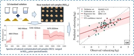
2.1. Experiment Framework

Figure 1 shows the entire study framework. As illustrated, the whole experiment process consists of three steps: (1) soil sampling, producing the NSS_Cd by adding standard Cd solution to background soil, and chemical analysis; (2) spectra measurement and pretreatment; and (3) model construction and validation. In this study, the near stand soil Cd samples (NSS_Cd) are proposed and defined as the samples with expected Cd concentration. The first step aims to collect the field soil samples from two case areas (i.e., Hengyang, Baoding), produce NSS_Cd with the background soil (i.e., unpolluted soil), and measure the Cd concentrations of all these soil samples. The second step, spectra measurement and pretreatment, involves measuring the hyperspectral signals of soil samples with a spectrometer and removing the random noise of the measured spectra. The third step involves the main process of the NSS spectra enhanced modeling strategy: the NSS_Cd prior spectral bands are extracted by the VIP method, and these spectral ranges are used to predict Cd concentration in NCS collected from the two case areas with both the CARS-PLS and PLS model.

2.2. Soil Sampling, Production and Chemical Analysis

2.2.1. Field soil Sampling

Two case areas are, respectively, located in southern Hengyang and northern Baoding in China (Figure 2a). The Hengyang study area is close to the Shuikoushan mining area at the upstream of the Xiangjiang river basin. The main soil type of this area is red soil, which contains Fe-oxides. The historic mining activities had discharged HM into the soil by chimneys exhaust, solid waste accumulation, and sewage [41]. The potential pollution is threatening the surrounding residents’ health. The Baoding study area is an agricultural land in Hebei province. This area is used as orchard and paddy field. Long-term irrigation and fertilization have led to the accumulate of heavy metal. The main soil type is loess.

In the Hengyang area, 57 naturally contaminated samples in topsoil (0–20 cm) were collected within the boundary from 112°35′24″ E to 113°36′37″ E and from 26°32′37″ N to 25°34′12″ N. These soil sampling sites are near the agricultural land, industrial land, and hydrology networks, etc. In the Baoding area, 42 naturally contaminated samples in topsoil (0–20 cm) within the boundary from 116°3′12″ E to 116°3′27″ E and from 38°55′38″ N to 38°36′30″ N were collected. These sampling sites are mainly located in the orchard and paddy field. Detailed spatial distribution of sampling sites are shown in Figure 2b,c. For each sample site, 500 g soil was collected and packed into plastic bags with a label, and the location was recorded by a global position system (GPS).

2.2.2. Near Standard Soil Cd Samples Production

To produce the NSS_Cd with Cd concentration ranges from low to high, the background soil must be unpolluted and homogenized. For this, we selected a high ground site in the neighbor of the Hengyang mining area, which was hardly polluted by mineral slag, sewage, etc. We collected about 30 kg of background soil from the same site. Furthermore, all of the background soil was stirred after plant residues and stones were eliminated.

After the pretreatment, five samples (each sample contains about 100 g) from the different parts of the whole background were used for chemical analysis in order to acquire their basic constituent information. The detailed process was the same as the description in Section 2.2.3. The average pH value of these background soils is 4.17, and the Cd concentration is 0.38 mg/kg, while the soil organic matter (SOM) is 6.78 g/kg. Detailed constituents are presented in Appendix A,

Table A1. pH value and constituents of NSS_Cd background soil and NCS.

Samples Set		pH	SOM (g/kg)	Fe (g/kg)	Cd (mg/kg)	Cu (mg/kg)	Pb (mg/kg)	As (mg/kg)
NSSCd background soil		4.17	6.78	21.03	0.38	16.50	26.10	9.77
Hengyang	Mean	5.49	42.22	50.17	28.85	259.73	2584.57	684.40
	SD	1.49	53.04	48.93	50.72	506.63	3647.29	1166.93
	CV	0.27	1.26	0.98	1.76	1.95	1.41	1.71
Baoding	Mean	8.17	86.42		0.35		123.31	8.85
	SD	0.21	26.76		0.06		46.52	2.70
	CV	0.03	0.31		0.17		0.38	0.31

. To make the expected concentrations of NSS_Cd correspond to a practical situation, it is necessary to consider the statistics of Cd concentrations in the previous investigations (Appendix A,

Table A2. Summary of Cd concentration in previous studies.

Sampling Area	Number of Sampling	Min	Max	Reference
Suburban area	44	0.32	0.51	[34]
Suburban area	93	0.22	0.64	[23]
Mining area	40	0.17	1.74	[61]
Mining area	70	0.17	34	[30]
Mining area	46	0.72	215.83	[3,29]
River sediments	117	0	18	[32]
Freshwater sediments	169	0.011	2.49	[31]
River sediments	150	0.022	0.08	[62]
Delta area	61	0.22	0.54	[10]
Delta area	122	0.081	1.441	[34]
Archaeological soil	11	0.07	0.11	[63]
Tailings polluted area	214	0.05	14.8	[12]

). In general, the Cd concentrations in soil are lower than 2 mg/kg. However, in mining areas, these concentrations are significantly higher and can even reach 200 mg/kg. Thus, the expected Cd concentrations of NSS_Cd were set from 0.5 to 54 mg/kg with the interval at 1 mg/kg. The interval of expected Cd concentrations was set to 0.1–0.2 mg/kg below 2 mg/kg.

Table 1. Cd concentrations expected and measured of near standard soil samples (mg/kg).

Sample No.	1	2	3	4	5	6	7	8	9	10	11	12	13
Expected	0.50	0.60	0.80	1.00	1.10	1.20	1.30	1.40	1.50	1.60	1.70	1.80	2.00
Measured	0.47	0.63	0.80	1.00	1.46	1.58	1.65	1.90	2.0	2.10	2.31	2.31	2.67
Sample No.	14	15	16	17	18	19	20	21	22	23	24	25	26
Expected	3.00	4.00	5.00	6.00	7.00	8.00	9.00	10.00	11.00	12.00	13.00	14.00	15.00
Measured	3.86	5.08	5.76	6.70	8.74	9.65	10.46	12.28	12.98	13.96	15.05	15.34	17.21
Sample No.	27	28	29	30	31	32	33	34	35	36	37	38	39
Expected	16.00	17.00	18.00	19.00	20.00	21.00	22.00	23.00	24.00	25.00	26.00	27.00	28.00
Measured	18.03	18.49	19.46	19.50	22.73	23.83	23.90	25.15	25.80	27.87	28.88	30.25	30.43
Sample No.	40	41	42	43	44	45	46	47	48	49	50	51	52
Expected	29.00	30.00	31.00	32.00	33.00	34.00	35.00	36.00	37.00	38.00	39.00	40.00	41.00
Measured	30.94	32.36	33.22	33.50	35.25	35.46	38.21	38.24	40.36	41.30	42.40	43.58	44.58
Sample No.	53	54	55	56	57	58	59	60	61	62	63	64	65
Expected	42.00	43.00	44.00	45.00	46.00	47.00	48.00	49.00	50.00	51.00	52.00	53.00	54.00
Measured	46.13	47.71	49.43	51.46	52.64	52.95	54.36	54.69	55.89	56.09	56.64	58.69	58.95

shows the final expected Cd concentrations of NSS_Cd.

Following the expected scheme of Table 1, each sample was individually made up of the C mL standard Cd solution (GSBG 62040-90(4801). Concentration, 1000 ug/L; Medium, 10% HCl) and 100 g of background soil and mixed thoroughly. The quantity of Cd solution (C) was calculated by Equation (1) [40]:

$$C={10}^{-3}\times \left(A-S\right)/\rho \times D,$$

(1)

where C represents the volume (mL) of the standard Cd solution adding into background soils samples; D represents the quantity of air-dried background soil samples without plant residues and stones (g), D = 100; A represents the expected concentrations of NSS_Cd (mg/kg) in Table 1; S represents the Cd concentration of the background soil (which is presented in Appendix A, Table A1); $\rho$ is the Cd concentration of standard Cd solution (mg/L), $\rho =1$. After that, all the NSS_Cd were settled for two months until the solution was naturally dried. Finally, this NSS_Cd could be used for the subsequent process.

In the NSS_Cd production process, there were measuring errors of the volume of Cd solution (C) and quantity of background (D). This was especially the case for D; while the soil was moved to the container after weighting, the quality was lost easily because of the residual soul on instruments. So, these factors inevitably lead to a deviation between the expected and actual Cd concentration of NSS_Cd. It was still necessary to verify the Cd concentration of NSS_Cd by chemical analysis.

2.2.3. Laboratory Chemical Analysis

Before the chemical analysis, all the NCS and NSS_Cd were pretreated in the following steps: (1) air-drying in the ventilated and shady place; (2) eliminating the plant residues and stones from the NCS; and (3) grinding by the agate mortar and sieving by using a 100-mesh polyethylene sieve. Then, a few soils were taken out from each sample and digested by the mixed-acid HNO₃-HF-HClO₄ in a microwave digestion instrument. Finally, Cd concentrations of soil samples were determined by atomic absorption spectrophotometry (AAS). The measurement accuracy of the soil Cd concentration is 0.03 mg/kg (GBT23739-2009), and the lowest detectable limit is at 0.005 mg/kg (GB15618-1995). Meanwhile, soil pH value was measured with a pH meter after shaking 10 g in a suspension of soil:water at a ratio of 1:5 for 30 min [42]. The whole process of soil samples chemical analysis was air-dried at the Soil and Fertilizer Institute in Hunan, China. The Cd concentration of NSS_Cd was present in Table 1. Detailed discussion about the difference of the measured values of Cd concentration of NSS_Cd were described in Section 2.2.2.

2.3. Spectra Measurement and Pretreatment

The instrument used for measuring spectra of soil samples in this study was the PSR-3500 spectrometer (Spectral Evolution Inc., Lawrence, MA, USA), covering a spectral range from 350 to 2500 nm. Spectral resolutions of the PSR-3500 spectrometer are 3.5 nm at 700 nm, 10 nm at 1500, and 7 nm at 2100 nm. The measurement process was carried out in a darkroom. After the pretreatment in Section 2.2.3, all the samples were placed on a black cloth in sample number order, while the top was smoothed down by lab spoon before spectra measurement. A 50 W halogen with a 30° zenith angle was used as the unique light source. The distance between the light source and the soil samples was 60 cm. The spectra of samples were calibrated by using a standardized white BaSO₄ panel before measuring every three samples. During the measurement process, the fiber optic probe was placed approximately 3 cm above the target soil sample and had a 45° zenith angle. Finally, each soil sample was scanned five times to measure the spectral reflectance, and the average spectrum was recorded.

For the measured spectra of soil samples, the spectral bands at intervals of 350–400 nm and 2400–2500 nm were, for the first, eliminated due to the low signal-to-noise ratio. Then, Savitzky–Golay smoothing with 15 points and second-order polynomials was adopted to filter and reduce the random noise of spectra. Additionally, outlier spectra caused by factors such as operation mistakes were further identified and removed using the spectral angle method, as these ‘outliers’ are significantly different from the normal soil spectra. The spectral angle is an index to evaluate the similarity between two spectra and can be calculated by the equation as follows:

$${\mathsf{\theta }}_{\mathrm{i}}=\mathrm{arcos}\frac{{{\displaystyle \sum }}_{\mathrm{j}=1}^{\mathrm{p}}{\mathrm{t}}_{\mathrm{j}}{\mathrm{r}}_{\mathrm{ij}}}{\sqrt{{{\displaystyle \sum }}_{\mathrm{j}=1}^{\mathrm{p}}{\mathrm{t}}_{\mathrm{j}}^2}\sqrt{{{\displaystyle \sum }}_{\mathrm{j}=1}^{\mathrm{p}}{\mathrm{r}}_{\mathrm{ij}}^2}},\mathrm{i}=1,2\cdots \mathrm{n},\mathsf{\theta }\in [0,\frac{\mathsf{\pi }}{2}],$$

(2)

where t_j represents the mean spectral reflectance in the j-th band of a set of samples; r_ij represents the spectral reflectance in the j-th band of the i-th sample; and p is the total number of spectral bands. If the θ_i is greater, there is a greater difference between the spectra of the i-th sample and the average spectra. The θ of all samples were analyzed by box plot. The first, third quartiles (Q₁ and Q₃), and the interquartile range (IQR = Q₃ − Q₁) were calculated. The samples which θ range outside the interval (Q₁ − 1.5 IQR, Q₃ + 1.5 IQR) are the outlier, the relevant spectrum can be regarded as error data. These samples were finally eliminated in this study.

2.4. Model Construction and Validation

2.4.1. Prior Spectral Bands Extraction

For the prior spectral bands, they were extracted with the VIP score of the PLS modeling [24,43]. The PLS model can be expressed as Equations (3) and (4) [44]:

$$\mathrm{X}={\mathrm{TP}}^{\mathrm{t}}+\mathrm{E}$$

(3)

$$\mathrm{y}=\mathrm{Tb}+\mathrm{f},$$

(4)

where, X (n × p) represents the spectra reflectance of n samples, p represents the number of bands, T (n × h) is the scores of h latent variables, P (p × h) is the loading matrix, and y (n × 1) is the concentration of HM. b (h × 1) is the regression coefficient of T. E (n × p) and f (n × 1) are the random error matrix. The result of the PLS model is influenced by the number of latent variables (h). The optimal PLS model was determined through the model performance, which is in detail described in Section 2.4.2.

VIP score refers to the variable importance in PLS projections. The idea is to accumulate the importance of each variable j being reflected by w from each component. In general, the variable j should be selected if ${\mathrm{VIP}}_{\mathrm{j}}>1$ [26]. Thus, in this study, the prior spectral bands were selected with this criterion. VIP score can be calculated based on the determined optimal PLS model as Equation (5) [25]:

$${\mathrm{VIP}}_{\mathrm{j}}=\sqrt{\mathrm{p}{{\displaystyle \sum }}_{\mathrm{k}=1}^{\mathrm{h}}(\mathrm{SS}\left({\mathrm{b}}_{\mathrm{k}}{\mathrm{t}}_{\mathrm{k}}\right){\left({\mathrm{w}}_{\mathrm{jk}}/\Vert {\mathrm{w}}_{\mathrm{k}}\Vert \right)}^2)/{{\displaystyle \sum }}_{\mathrm{k}=1}^{\mathrm{h}}\mathrm{SS}\left({\mathrm{b}}_{\mathrm{k}}{\mathrm{t}}_{\mathrm{k}}\right)}$$

(5)

2.4.2. Model Calibration and Validation

The PLS model is the primary method employed to predict soil HM using VNIR spectroscopy technology due to its the ability to process the data in which the number of variables greatly exceeded the number of samples (especially multicollinearity data) [45]. On this basis, as an advanced variable selection technique, CARS can improve the original PLS model [17]. The process of CARS contains the N times iterative sampling of subset bands of spectral. In this study, N was set to 100. Each subset bands of spectral sampling from the NCS based includes the following steps: (1) choosing k subset bands of spectral samples from the calibration set by Monte Carlo to build PLS model and evaluating the importance of each spectral band by normalized weight; (2) reducing the number of model variables (i.e., subset bands of spectral) with the adaptive reweighted sampling method and finalizing the number with exponentially decreasing function; (3) repeating step 1 and step 2 until the sampling times reached N; and (4) determining the optimal variable selection while the root mean square error of leave-one-out cross-validation (RMSECV) is the minimum. Figure 3 presents the process of the CARS variable selection. While the RMSECV is the minimum, the optimal variable selection is determined and it is marked with a vertical line in the third-row subfigures. The CARS algorithm was performed in the libPLS package (download from www.libpls.net, [21], accessed on 26 December 2018). PLS and CARS-PLS models were carried out in MATLAB 2016a.

The NSS spectra enhanced modeling strategy was proposed in this study. The VIP scores of NSS_Cd spectra band were calculated with Equation (5). The NSS prior spectral bands were selected with the criterion “$\mathrm{VIP}>1$”, and these bands were used to predict Cd concentration in NCS. The CARS-PLS and PLS model were carried out the NSS spectra enhanced modeling strategy (CARS-PLS_NSS-VIP-VNIR and PLS_NSS-VIP-VNIR). To verify the effectiveness of the proposed modeling strategy, the conventional method of predicting Cd concentration using the entire VNIR was the contrast experiment (CARS-PLS_VNIR and PLS_VNIR).

To verify the stability of the NSS_Cd spectra enhanced modeling strategy, the calibration and validation set of models were selected every one in five samples (i.e., 1/5 of total samples) while the samples were sorted in ascending Cd concentration. The rest of the soil samples were used as a calibration (i.e., training) set. This method can ensure that the concentration of calibration and validation sets distribute similarly [3]. The number of the validation set can be also set to 1/4, 1/3, and 1/2 of the total samples in the model validation.

As redundant latent variables will result in overfitting, leave-one-out cross-validation was used to determine the optimal number of latent variables (LVs) of PLS according to the following criterion: the later LV will refuse to be added while the improvement of RMSECV is less than 4% [3].

For the precision evaluation of the CARS-PLS_NSS-VIP-VNIR and PLS_NSS-VIP-VNIR models, the determination coefficient (R²), root mean square error of prediction (RMSEP), and the ratio of prediction to deviation (RPD) was used. A reliable model is supposed to have high R², low RMSE, and high RPD. RPD is defined as the ratio of the standard deviation of the data set to RMSEP:

$$\mathrm{RPD}=\mathrm{SD}/\mathrm{RMSEP}$$

(6)

3. Results

3.1. Cd Concentration Statistics of Soil Samples

The statistics of soil samples Cd concentrations are presented in

Table 2. Statistics of Cd concentrations (mg/kg) of different sample sets.

Samples Set	Min	Max	Mean	SD	CV
Hengyang (n = 57)	0.72	215.83	25.07	45.55	1.82
Baoding (n = 42)	0.27	0.50	0.35	0.05	0.15
NSSCd (n = 65)	0.47	58.95	25.91	18.31	0.71

pH value is 5.5, 8.5, and 4.17 for Hengyang, Baoding, and NSS_Cd.

. The minimum and maximum Cd concentrations are 0.72 mg/kg and 215.83 mg/kg in the Hengyang soil samples, and 0.27 mg/kg and 0.50 mg/kg in the Baoding soil samples, respectively. The standard deviation (SD) of samples in Hengyang and Baoding is 45.55 mg/kg and 0.05 mg/kg, respectively. To eliminate the effects of measurement scale and dimension, the coefficient of variation (CV) values, a non-dimensional quantity, was calculated to evaluate the degree of variation of Cd concentration. The Cd concentration CV values of samples in Hengyang and Baoding are 0.78 and 0.15, respectively. For the NSS_Cd, the range of Cd concentration is 0.47–58.95 mg/kg, and the CV value is 0.71. The detailed values are presented in Table 1. With the factor mentioned in Section 2.2.2, the measured values are 10% higher than the expected values. However, they are mainly consistent with the expected values in Table 1, which is acceptable for being used to analyze in model construction.

According to the Environmental Quality Standard for Soils (GB 15618-1995) published by the Ministry of Environmental Protection of China, the tolerable value is 0.3 mg/kg for soils with pH ≤ 6.5 and 0.6 mg/kg for soils with pH ≥ 6.5. The Cd concentrations of all of the soil samples in Hengyang exceed the tolerable value. It indicates that there is serious contamination in Hengyang. In contrast, the Cd concentrations of all of the soil samples in Baoding were below the tolerable value. The data should be normal distribution for modeling, and the Kolmogorov–Smirnov method was used to test the distribution. The Cd concentration of samples in Hengyang is a skewed distribution because of the high value of Cd concentration in several of the samples. Therefore, in the latter, the box-cox transform was used to correct for data distribution. The Cd concentration of samples in Baoding is s normal distribution, which does not require transformation.

3.2. Spectral Response Characteristics of Soil Samples

The spectra of soil samples were presented in Figure 4. According to Figure 4, for all of the samples, there are four main absorptions around 900 nm, 1400 nm, 1900 nm, and 2200 nm. The absorption around 1400 nm and 1900 nm are caused by hydroxyl functional groups of free water [46,47], and the absorption around 2200 nm is caused by the clay lattice Al–OH [48,49,50]. However, there are obvious differences between the spectra curve of three sample sets.

For the NCS in the Hengyang study area, the depth of absorptions is greater than the NCS in Baoding, which is caused by the abundant ferric and aluminum oxide in red soil. Additionally, the spectra of samples in Hengyang are various because the samples were collected from different sites in mine tailing, farmland, factories, etc. The NCS in the Baoding study area were all collected from agricultural land (according to Appendix A Table A1) and all of the degrees of variation of soil constituents are lower than samples in Hengyang. The soil texture is relatively unitary, so the spectral curves are uniform.

Compared to the NCS, the NSS_Cd spectra are more uniform in shape because of the production with the same background soil. All constituents are the same except for the Cd concentration. The Cd concentration is the only factor which influenced the spectra of NSS_Cd, This situation is similar to the samples in Baoding. The increasing trend of spectral reflectance in the visible range and the depth of absorptions are similar to some of the samples in the Hengyang study area. It is probably due to the fact that the soil type of background soil is similar to the NCS in Hengyang.

3.3. Prior Spectral Bands Extraction from NSS_Cd

For NSS_Cd, the optimal precision of predicting Cd concentration is presented as follows: The ${\mathrm{R}}^2$, RMSE with PLS model are 0.78, 9.33, and RPD = 2.05. The model is reliable. The PLS model regression coefficient and VIP score for each band are presented in Figure 5. According to the criterion “VIP > 1” mentioned in Section 2.4.1, the prior spectral bands extracted from NSS_Cd are mainly in the range of 400–570 nm, 940–990 nm, 1390–1430 nm, and 1670–2020 nm. In previous studies, several spectral bands with high correlation to Cd concentration were found, including bands around 540 nm [51], 490–580 nm [31], 1000 nm [29], 1400 nm [52], and 2000 nm [24]. The prior spectral bands of NSS_Cd covers the results in previous studies. The variety of NSS_Cd spectra is almost caused by Cd concentration. Therefore, these prior spectral bands imply general spectral response characteristics and are used to enhance the Cd concentration prediction in NCS.

3.4. Prediction Precision of NSS_Cd Enhanced Model

The RMSECV against the number of LVs is shown in Figure 6, which determines the optimal number of LVs (validation set ratio = 1/5). In Figure 6a, the RMSECV is the local minimum while the number of LVs is 3. With the increase of LVs, the RMSECV is decreased by less than 4%. According to the criterion in Section 2.4.2, the latter added LVs is unnecessary. The optimal number of LVs for Hengyang is 3. In Figure 6b, the RMSECV decreases sharply while the number of LVs increasing to 3 for the CARS-PLS_VNIR model and reached the minimum while LVs is 4 for the CARS-PLS_NSS-VIP-VNIR. For the PLS_NSS-VIP-VNIR and PLS_VNIR, while the 6th LV was added, the decrease of RMSECV is less than 4%. The optimal number of LVs is regarded as 5. The optimal number of LVs can be determined in the same way while the validation ratio changed, and the results are presented in

Table 3. Prediction precision of PLS_NSS-VIP-VNIR, CARS-PLS_NSS-VIP-VNIR, PLS_VNIR, and CARS-PLS_VNIR models.

Sample Set	The Ratio of the Validation Set	Model	LVs	RMSEP	R2p	RPD	Model	LVs	RMSEP	R2p	RPD
Hengyang	1/5 (n = 11)	PLSNSS-VIP-VNIR	3	0.555	0.71	1.95	CARS-PLSNSS-VIP-VNIR	3	0.610	0.65	1.77
	1/4 (n = 14) *		3	0.646	0.60	1.65		3 *	0.656 *	0.59 *	1.62
	1/3 (n = 19)		3	0.565	0.67	1.78		4	0.545	0.69	1.84
	1/2 (n = 28)		3	0.618	0.57	1.55		3	0.651	0.52	1.47
	1/5 (n = 11)	PLSVNIR	3	0.626	0.63	1.72	CARS-PLSVNIR	3	0.790	0.41	1.37
	1/4 (n = 14)		3	0.703	0.53	1.51		3	0.609	0.65	1.75
	1/3 (n = 19)		3	0.651	0.56	1.55		3	0.668	0.53	1.50
	1/2 (n = 28)		3	0.632	0.55	1.51		6	0.661	0.50	1.45
Baoding	1/5 (n = 8)	PLSNSS-VIP-VNIR	5	0.029	0.68	1.90	CARS-PLSNSS-VIP-VNIR	4	0.025	0.76	2.19
	1/4 (n = 10)		5	0.028	0.65	1.79		5	0.036	0.42	1.39
	1/3 (n = 14)		3	0.037	0.38	1.33		5	0.049	0.32	1.27
	1/2 (n = 21) *		5	0.030	0.59	1.60		6 *	0.031 *	0.54 *	1.51 *
	1/5 (n = 8)	PLSVNIR	5	0.033	0.59	1.66	CARS-PLSVNIR	3	0.035	0.54	1.57
	1/4 (n = 10)		3	0.030	0.60	1.68		5	0.041	0.25	1.23
	1/3 (n = 14)		4	0.040	0.30	1.25		3	0.051	0.26	1.21
	1/2 (n = 21)		3	0.032	0.53	1.50		4	0.030	0.59	1.60

The cases that the NSS_Cd enhanced models get higher precision than using entire VNIR were marked with bold font. And the exceptional cases were marked with *.

.

The results of the NSS_Cd enhanced models (PLS_NSS-VIP-VNIR and CARS-PLS_NSS-VIP-VNIR) are presented in Table 3. As a comparison, prediction precision that using the entire VNIR (PLS_VNIR and CARS-PLS_VNIR model) is also presented. The higher precision is marked with bold font. Figure 7 and Figure 8 are the scatter plots of the observed against predicted Cd concentration. The red dots and green dots represent the validation and calibration set respectively. The 95% confidence interval of regression line is marked with a red shaded region.

For the Hengyang sample set, while the validation set ratio is set to 1/5, compared to the PLS_VNIR model, the ${\mathrm{R}}_{\mathrm{p}}^2$, RPD of the PLS_NSS-VIP-VNIR model are improved from 0.63 and 1.72 to 0.71 and 1.95. A similar improvement is also found in comparing the CARS-PLS_NSS-VIP-VNIR and CARS-PLS_VNIR model, the ${\mathrm{R}}_{\mathrm{p}}^2$, RPD are improved from 0.41 and 1.37 to 0.65 and 1.77. For the Baoding sample set, the ${\mathrm{R}}_{\mathrm{p}}^2$, RPD of the PLS_NSS-VIP-VNIR model are improved to from 0.59 and 1.66 to 0.68 and 1.90 compared to the PLS_VNIR model. And the ${\mathrm{R}}_{\mathrm{p}}^2$, RPD of the CARS-PLS_NSS-VIP-VNIR model are improved from 0.54 and 1.57 to 0.76 and 2.19 compared to the CARS-PLS_VNIR model. With the validation set ratio changed to 1/4, 1/3, and 1/2, the NSS_Cd enhanced model still gets higher precision than using the entire VNIR in most cases. However, even if for the exceptional cases (which marked with * in Table 3), the prediction precision is still reliable.

In addition, other sample selection method such as Kennard–Stone (KS) is also widely utilized in soil spectroscopy for selecting calibration [53,54]. The results of the NSS enhanced model which validation set is selected by the KS algorithm are presented in Appendix A,

Table A3. Supplyment result of RF model while the validation set was selected (1) every 1 in 5 samples with the ascending sorted Cd concentration; (2) Kennard-Stone algorithm (1/5 of sample set).

Sample Set	Selected Validation Set	PLSNSS-VIP-VNIR			CARS-PLSNSS-VIP-VNIR			RFNSS-VIP-VNIR
		RMSEP	R2p	RPD	RMSEP	R2p	RPD	RMSEP	R2p	RPD
Hengyang	(1)	0.555	0.71	1.95	0.610	0.65	1.77	0.661	0.59	1.63
	(2)	0.618	0.40	1.36	0.622	0.40	1.35	0.411	0.45	1.42
Baoding	(1)	0.029	0.68	1.90	0.025	0.76	2.19	0.034	0.42	1.42
	(2)	0.050	0.53	1.58	0.053	0.48	1.50	0.059	0.36	1.35

. Comparing to the results in Table 3, the results which validation selected by KS is lower (${\mathrm{R}}_{\mathrm{p}}^2$ is ranged in 0.36–0.53). The KS method can ensure that the distribution of calibration is uniform to the total samples along the spectra. This perhaps leads to the difference distribution of Cd concentration between calibration and validation sets since the sample number is not large enough. Unlike the KS method, the method that selected every one in five samples with the ascending sorted Cd concentration ensure that the distribution of calibration is uniform to the total samples along the Cd concentration.

4. Discussion

To eliminate the influence on spectra caused by heterogeneous soil [35], NSS_Cd were produced to reveal the soil’s Cd spectral response characteristics. Considering the redundant information of the entire VNIR [17], the NSS_Cd prior spectral bands were extracted by VIP scores, which are mainly ranged in 400–570 nm, 940–990 nm, 1390–1430 nm, and 1670–2020 nm. These spectral ranges are the union of spectral response characteristics of Cd concentration in previous studies [24,31,51,52]. Thus, these spectral ranges are more universal.

According to the results of soil Cd concentration prediction, the use of NSS_Cd prior spectral bands can improve the prediction precision of Cd concentration. In Table 3, the ${\mathrm{R}}_{\mathrm{p}}^2$, RPD and RMSE were improved 9%, 16%, and 11% on average. The ${\mathrm{R}}_{\mathrm{p}}^2$ and RPD were improved, most significantly from 0.41 and 1.37 to 0.65 and 1.77 for Hengyang sample set, and improved from 0.54 and 1.57 to 0.76 and 2.19 for the Baoding sample set. The two exceptional cases marked with * in Table 3. For the CARS-PLS_NSS-VIP-VNIR model, the ${\mathrm{R}}_{\mathrm{p}}^2$ were respectively decreased from 0.65 and 0.59 to 0.59 and 0.54 in Hengyang (validation set ratio = 1/4) and Baoding (validation set ratio = 1/2), respectively. The CARS method can be influenced by the variety of training sets when the sample number is not large enough. It perhaps this reason that led to these two exceptional cases. However, the prediction is still reliable in these cases. It indicates that the NSS_Cd enhanced model is effective in general.

Though the band number of NSS_Cd prior spectral bands is significantly less than the entire VNIR, these bands perhaps contain the main spectral information for predicting Cd concentration and have the potential to reveal spectral response characteristics. Some previous studies have proposed that there is redundant information in the entire VNIR, and that using subset bands of spectra represents an effective method for improving soil HM prediction [3].

Additionally, in this study, NSS_Cd prior spectral bands extracted by VIP scores were more effective than the band selected by the CARS method. It was noticed that the precision of the CARS-PLS_VNIR is lower than the PLS_NSS-VIP-VNIR model both for the NCS in Hengyang and Baoding. In some cases, the CARS method was useless for improving precision. For example, the PLS_NSS-VIP-VNIR model gets higher precision than the CARS-PLS_NSS-VIP-VNIR model when the validation set ratio is 1/4 and 1/2, respectively. As a variable selection method, CARS can eliminate uninformative variables based on weight. However, the results of variable selection are perhaps influenced by the spectra variation caused by heterogeneous soil. The spectra bands selected by the CARS method are inconsistent in different areas, which may possibly lead to controversial spectral bands for predicting soil HM as in previous studies. In contrast, the NSS_Cd prior spectral bands are extracted based on the prior knowledge of NSS_Cd spectra, which are more likely to reveal the spectral characteristic of soil Cd. This is the main reason that NSS_Cd prior spectral bands are more effective in predicting Cd concentration than spectra bands selected by the CARS method. Therefore, the NSS_Cd prior spectral bands can be widely applied to predict Cd concentration in different areas.

Moreover, an NSS enhanced model based on machine learning was also carried out. Random forest (RF) is popular in spectral reflectance due to the accuracy of its classifications [55,56]. It is also applicable to regression and used in some cases [57,58,59]. The result of the RF_NSS-VIP-VNIR model is presented in Appendix A, Table A3. However, the precision of the RF_NSS-VIP-VNIR model is lower than the PLS_NSS-VIP-VNIR and CARS-PLS_NSS-VIP-VNIR models. Machine learning is suitable for non-linear regression problems with a large number of samples. However, in this study, due to limitation of the number of samples, machine learning did not perform well. However, for the large number samples, it is worth exploring the capability of the NSS enhance model combined with machine learning for further study.

In this study, although NSS_Cd prior spectral bands can be applied to these two areas, it does not mean that it can be applied to all possible study areas. Because soil type is an important factor which can influence spectra, it is necessary to verify the applicability of the NSS_Cd spectra enhanced modeling strategy on more types of soil. In addition, the mechanism for predicting soil HM concentration using VNIR spectroscopy is based on HM adsorption on Fe-oxides, clays, and SOM. Therefore, while the other constituent concentrations (e.g., SOM, clays, etc.) of background soil are varied, it is uncertain whether the result of prior spectral bands extracted by VIP scores from NSS_Cd will differ from the result in this paper. Moreover, considering the high Cd concentration range of NSS_Cd (0.47–58.95 mg/kg), it is difficult to ensure NSS_Cd prior spectral bands’ reliability for NCS with a low Cd concentration.

For this reason, in further studies, the producing NSS with heterogeneous background soil should be produced to reveal the spectral response characteristic of HM in heterogeneous soil (e.g., the NSS produced based on soil with a high SOM and low SOM concentration). The proposed NSS_Cd spectra enhanced modeling strategy also should be used in more study areas with different soil types to verify its’ transferability [60]. For other types of soil HM, the spectral characteristics also can reveal by this method. These NSS prior spectral bands are significant for the development of sensors for detecting soil HM. It is a promising hyperspectral remote sensing technique for rapidly detecting soil HM concentrations on a large scale.

5. Conclusions

• The NSS_Cd spectra enhanced modeling strategy can effectively predict Cd concentration in different areas.
• NSS_Cd prior spectral bands are important for the selection of spectral response characteristics from VNIR of natural soil samples.
• The VIP method is more helpful to select the key band for predicting Cd concentration than the CARS method.

References

1. Cao, S.; Duan, X.; Zhao, X.; Ma, J.; Dong, T.; Huang, N.; Sun, C.; He, B.; Wei, F. Health Risks from the Exposure of Children to As, Se, Pb and Other Heavy Metals near the Largest Coking Plant in China. Sci. Total Environ. 2014, 472, 1001–1009. [Google Scholar] [CrossRef]
2. Wu, Z.; Chen, Y.; Han, Y.; Ke, T.; Liu, Y. Identifying the Influencing Factors Controlling the Spatial Variation of Heavy Metals in Suburban Soil Using Spatial Regression Models. Sci. Total Environ. 2020, 717, 137212. [Google Scholar] [CrossRef]
3. Zhang, X.; Sun, W.; Cen, Y.; Zhang, L.; Wang, N. Predicting Cadmium Concentration in Soils Using Laboratory and Field Reflectance Spectroscopy. Sci. Total Environ. 2019, 650, 321–334. [Google Scholar] [CrossRef]
4. Jiang, X.; Zou, B.; Feng, H.; Tang, J.; Tu, Y.; Zhao, X. Spatial Distribution Mapping of Hg Contamination in Subclass Agricultural Soils Using GIS Enhanced Multiple Linear Regression. J. Geochem. Explor. 2019, 196, 1–7. [Google Scholar] [CrossRef]
5. Khosravi, V.; Doulati Ardejani, F.; Yousefi, S.; Aryafar, A. Monitoring Soil Lead and Zinc Contents via Combination of Spectroscopy with Extreme Learning Machine and Other Data Mining Methods. Geoderma 2018, 318, 29–41. [Google Scholar] [CrossRef]
6. Achary, M.S.; Satpathy, K.K.; Panigrahi, S.; Mohanty, A.K.; Padhi, R.K.; Biswas, S.; Prabhu, R.K.; Vijayalakshmi, S.; Panigrahy, R.C. Concentration of Heavy Metals in the Food Chain Components of the Nearshore Coastal Waters of Kalpakkam, Southeast Coast of India. Food Control 2017, 72, 232–243. [Google Scholar] [CrossRef]
7. Chen, R.; de Sherbinin, A.; Ye, C.; Shi, G. China’s Soil Pollution: Farms on the Frontline. Science 2014, 344, 691. [Google Scholar] [CrossRef] [PubMed]
8. Zou, B.; Jiang, X.; Duan, X.; Zhao, X.; Zhang, J.; Tang, J.; Sun, G. An Integrated H-G Scheme Identifying Areas for Soil Remediation and Primary Heavy Metal Contributors: A Risk Perspective. Sci. Rep. 2017, 7, 341. [Google Scholar] [CrossRef]
9. Wang, F.; Gao, J.; Zha, Y. Hyperspectral Sensing of Heavy Metals in Soil and Vegetation: Feasibility and Challenges. ISPRS J. Photogramm. Remote Sens. 2018, 136, 73–84. [Google Scholar] [CrossRef]
10. Wu, Y.; Chen, J.; Ji, J.; Gong, P.; Liao, Q.; Tian, Q.; Ma, H. A Mechanism Study of Reflectance Spectroscopy for Investigating Heavy Metals in Soils. Soil Sci. Soc. Am. J. 2007, 71, 918–926. [Google Scholar] [CrossRef]
11. Jiang, Q.; Liu, M.; Wang, J.; Liu, F. Feasibility of Using Visible and Near-Infrared Reflectance Spectroscopy to Monitor Heavy Metal Contaminants in Urban Lake Sediment. Catena 2018, 162, 72–79. [Google Scholar] [CrossRef]
12. Kemper, T.; Sommer, S. Estimate of Heavy Metal Contamination in Soils after a Mining Accident Using Reflectance Spectroscopy. Environ. Sci. Technol. 2002, 36, 2742–2747. [Google Scholar] [CrossRef] [PubMed]
13. Tan, K.; Wang, H.; Zhang, Q.; Jia, X. An Improved Estimation Model for Soil Heavy Metal(Loid) Concentration Retrieval in Mining Areas Using Reflectance Spectroscopy. J. Soils Sediments 2018, 18, 2008–2022. [Google Scholar] [CrossRef]
14. Tu, Y.L.; Zou, B.; Jiang, X.L.; Tao, C.; Feng, H.H. Hyperspectral Remote Sensing Based Modeling of Cu Content in Mining Soil. Spectrosc. Spectr. Anal. 2018, 38, 575–581. [Google Scholar]
15. Yousefi, G.; Homaee, M.; Norouzi, A.A. Estimating Soil Heavy Metals Concentration at Large Scale Using Visible and Near-Infrared Reflectance Spectroscopy. Env. Monit. Assess 2018, 190, 513. [Google Scholar] [CrossRef]
16. Tan, K.; Ma, W.; Chen, L.; Wang, H.; Du, Q.; Du, P.; Yan, B.; Liu, R.; Li, H. Estimating the Distribution Trend of Soil Heavy Metals in Mining Area from HyMap Airborne Hyperspectral Imagery Based on Ensemble Learning. J. Hazard. Mater. 2021, 401, 123288. [Google Scholar] [CrossRef] [PubMed]
17. Li, H.; Liang, Y.; Xu, Q.; Cao, D. Key Wavelengths Screening Using Competitive Adaptive Reweighted Sampling Method for Multivariate Calibration. Anal. Chim. Acta 2009, 648, 77–84. [Google Scholar] [CrossRef]
18. Hong, Y.; Chen, Y.; Yu, L.; Liu, Y.; Liu, Y.; Zhang, Y.; Liu, Y.; Cheng, H. Combining Fractional Order Derivative and Spectral Variable Selection for Organic Matter Estimation of Homogeneous Soil Samples by VIS–NIR Spectroscopy. Remote Sens. 2018, 10, 479. [Google Scholar] [CrossRef] [Green Version]
19. Huang, X.; Luo, Y.-P.; Xu, Q.-S.; Liang, Y.-Z. Elastic Net Wavelength Interval Selection Based on Iterative Rank PLS Regression Coefficient Screening. Anal. Methods 2017, 9, 672–679. [Google Scholar] [CrossRef]
20. Sun, W.; Zhang, X. Estimating Soil Zinc Concentrations Using Reflectance Spectroscopy. Int. J. Appl. Earth Obs. Geoinf. 2017, 58, 126–133. [Google Scholar] [CrossRef]
21. Sun, W.; Zhang, X.; Sun, X.; Sun, Y.; Cen, Y. Predicting Nickel Concentration in Soil Using Reflectance Spectroscopy Associated with Organic Matter and Clay Minerals. Geoderma 2018, 327, 25–35. [Google Scholar] [CrossRef]
22. Liu, Y.; Chen, Y. Estimation of Total Iron Content in Floodplain Soils Using VNIR Spectroscopy—A Case Study in the Le’an River Floodplain, China. Int. J. Remote Sens. 2012, 33, 5954–5972. [Google Scholar] [CrossRef]
23. Choe, E.; van der Meer, F.; van Ruitenbeek, F.; van der Werff, H.; de Smeth, B.; Kim, K.-W. Mapping of Heavy Metal Pollution in Stream Sediments Using Combined Geochemistry, Field Spectroscopy, and Hyperspectral Remote Sensing: A Case Study of the Rodalquilar Mining Area, SE Spain. Remote Sens. Environ. 2008, 112, 3222–3233. [Google Scholar] [CrossRef]
24. Cheng, H.; Shen, R.; Chen, Y.; Wan, Q.; Shi, T.; Wang, J.; Wan, Y.; Hong, Y.; Li, X. Estimating Heavy Metal Concentrations in Suburban Soils with Reflectance Spectroscopy. Geoderma 2019, 336, 59–67. [Google Scholar] [CrossRef]
25. Chong, I.-G.; Jun, C.-H. Performance of Some Variable Selection Methods When Multicollinearity Is Present. Chemom. Intell. Lab. Syst. 2005, 78, 103–112. [Google Scholar] [CrossRef]
26. Mehmood, T.; Liland, K.H.; Snipen, L.; Sæbø, S. A Review of Variable Selection Methods in Partial Least Squares Regression. Chemom. Intell. Lab. Syst. 2012, 118, 62–69. [Google Scholar] [CrossRef]
27. Pallottino, F.; Stazi, S.R.; D’Annibale, A.; Marabottini, R.; Allevato, E.; Antonucci, F.; Costa, C.; Moscatelli, M.C.; Menesatti, P. Rapid Assessment of As and Other Elements in Naturally-Contaminated Calcareous Soil through Hyperspectral VIS-NIR Analysis. Talanta 2018, 190, 167–173. [Google Scholar] [CrossRef]
28. Shi, T.; Liu, H.; Wang, J.; Chen, Y.; Fei, T.; Wu, G. Monitoring Arsenic Contamination in Agricultural Soils with Reflectance Spectroscopy of Rice Plants. Environ. Sci. Technol. 2014, 48, 6264–6272. [Google Scholar] [CrossRef] [PubMed]
29. Zou, B.; Long, T.Y.; Jiang, X.L.; Tao, C.; Zhou, M.; Xiong, L.W. Estimation of Cd Content in Soil Using Combined Laboratory and Field DS Spectroscopy. Spectrosc. Spectr. Anal. 2019, 39, 3223–3231. [Google Scholar]
30. Lü, J.; Jiao, W.-B.; Qiu, H.-Y.; Chen, B.; Huang, X.-X.; Kang, B. Origin and Spatial Distribution of Heavy Metals and Carcinogenic Risk Assessment in Mining Areas at You’xi County Southeast China. Geoderma 2018, 310, 99–106. [Google Scholar] [CrossRef]
31. Siebielec, G.; McCarty, G.W.; Stuczynski, T.I.; Reeves, J.B. Near- and Mid-Infrared Diffuse Reflectance Spectroscopy for Measuring Soil Metal Content. J. Environ. Qual. 2004, 33, 2056–2069. [Google Scholar] [CrossRef] [Green Version]
32. Malley, D.F.; Williams, P.C. Use of Near-Infrared Reflectance Spectroscopy in Prediction of Heavy Metals in Freshwater Sediment by Their Association with Organic Matter. Environ. Sci. Technol. 1997, 31, 3461–3467. [Google Scholar] [CrossRef]
33. Moros, J.; de Vallejuelo, S.F.-O.; Gredilla, A.; de Diego, A.; Madariaga, J.M.; Garrigues, S.; de la Guardia, M. Use of Reflectance Infrared Spectroscopy for Monitoring the Metal Content of the Estuarine Sediments of the Nerbioi-Ibaizabal River (Metropolitan Bilbao, Bay of Biscay, Basque Country). Environ. Sci. Technol. 2009, 43, 9314–9320. [Google Scholar] [CrossRef]
34. Song, Y.; Li, F.; Yang, Z.; Ayoko, G.A.; Frost, R.L.; Ji, J. Diffuse Reflectance Spectroscopy for Monitoring Potentially Toxic Elements in the Agricultural Soils of Changjiang River Delta, China. Appl. Clay Sci. 2012, 64, 75–83. [Google Scholar] [CrossRef]
35. Horta, A.; Malone, B.; Stockmann, U.; Minasny, B.; Bishop, T.F.A.; McBratney, A.B.; Pallasser, R.; Pozza, L. Potential of Integrated Field Spectroscopy and Spatial Analysis for Enhanced Assessment of Soil Contamination: A Prospective Review. Geoderma 2015, 241–242, 180–209. [Google Scholar] [CrossRef] [Green Version]
36. Ferrer, M.L.; Lawrence, C.; Demirjian, B.G.; Kivelson, D.; Alba-Simionesco, C.; Tarjus, G. Supercooled Liquids and the Glass Transition: Temperature as the Control Variable. J. Chem. Phys. 1998, 109, 8010–8015. [Google Scholar] [CrossRef]
37. Pelta, R.; Ben-Dor, E. Assessing the Detection Limit of Petroleum Hydrocarbon in Soils Using Hyperspectral Remote-Sensing. Remote Sens. Environ. 2019, 224, 145–153. [Google Scholar] [CrossRef]
38. Zhang, S.; Li, J.; Wang, S.; Huang, Y.; Li, Y.; Chen, Y.; Fei, T. Rapid Identification and Prediction of Cadmium-Lead Cross-Stress of Different Stress Levels in Rice Canopy Based on Visible and Near-Infrared Spectroscopy. Remote Sens. 2020, 12, 469. [Google Scholar] [CrossRef] [Green Version]
39. Jiang, X.L.; Zou, B.; Tu, Y.L.; Feng, H.H.; Chen, X. Quantitative Estimation of Cd Concentrations of Type Standard Soil Samples Using Hyperspectral Data. Spectrosc. Spectr. Anal. 2018, 38, 3254–3260. [Google Scholar]
40. Zou, B.; Jiang, X.; Feng, H.; Tu, Y.; Tao, C. Multisource Spectral-Integrated Estimation of Cadmium Concentrations in Soil Using a Direct Standardization and Spiking Algorithm. Sci. Total Environ. 2020, 701, 134890. [Google Scholar] [CrossRef]
41. Wei, C.; Wang, C.; Yang, L. Characterizing Spatial Distribution and Sources of Heavy Metals in the Soils from Mining-Smelting Activities in Shuikoushan, Hunan Province, China. J. Environ. Sci. 2009, 21, 1230–1236. [Google Scholar] [CrossRef]
42. Briki, M.; Ji, H.; Li, C.; Ding, H.; Gao, Y. Characterization, Distribution, and Risk Assessment of Heavy Metals in Agricultural Soil and Products around Mining and Smelting Areas of Hezhang, China. Env. Monit. Assess 2015, 187, 767. [Google Scholar] [CrossRef] [PubMed]
43. Xu, D.; Chen, S.; Viscarra Rossel, R.A.; Biswas, A.; Li, S.; Zhou, Y.; Shi, Z. X-ray Fluorescence and Visible near Infrared Sensor Fusion for Predicting Soil Chromium Content. Geoderma 2019, 352, 61–69. [Google Scholar] [CrossRef]
44. Wold, S.; Sjöström, M.; Eriksson, L. PLS-Regression: A Basic Tool of Chemometrics. Chemom. Intell. Lab. Syst. 2001, 58, 109–130. [Google Scholar] [CrossRef]
45. Shi, T.; Chen, Y.; Liu, Y.; Wu, G. Visible and Near-Infrared Reflectance Spectroscopy—An Alternative for Monitoring Soil Contamination by Heavy Metals. J. Hazard. Mater. 2014, 265, 166–176. [Google Scholar] [CrossRef]
46. Shepherd, K.D.; Walsh, M.G. Development of Reflectance Spectral Libraries for Characterization of Soil Properties. Soil Sci. Soc. Am. J. 2002, 66, 988–998. [Google Scholar] [CrossRef]
47. Stoner, E.R.; Baumgardner, M.F. Characteristic Variations in Reflectance of Surface Soils. Soil Sci. Soc. Am. J. 1981, 45, 1161–1165. [Google Scholar] [CrossRef] [Green Version]
48. Ben-Dor, E.; Banin, A. Near-Infrared Analysis as a Rapid Method to Simultaneously Evaluate Several Soil Properties. Soil Sci. Soc. Am. J. 1995, 59, 364–372. [Google Scholar] [CrossRef]
49. Clark, R.N.; King, T.V.V.; Klejwa, M.; Swayze, G.A.; Vergo, N. High Spectral Resolution Reflectance Spectroscopy of Minerals. J. Geophys. Res. 1990, 95, 12653. [Google Scholar] [CrossRef] [Green Version]
50. Viscarra Rossel, R.A.; McGlynn, R.N.; McBratney, A.B. Determining the Composition of Mineral-Organic Mixes Using UV–Vis–NIR Diffuse Reflectance Spectroscopy. Geoderma 2006, 137, 70–82. [Google Scholar] [CrossRef]
51. Gu, Y.W.; Li, S.; Gao, W.; Wei, H. Hyperspectral Estimation of the Cadmium Content in Leaves of Brassica Rapa Chinesis Based on the Spectral Parameters. Acta Ecol. Sin. 2015, 35, 4445–4453. [Google Scholar]
52. Kooistra, L.; Wehrens, R.; Leuven, R.S.E.W.; Buydens, L.M.C. Possibilities of Visible–near-Infrared Spectroscopy for the Assessment of Soil Contamination in River Floodplains. Anal. Chim. Acta 2001, 446, 97–105. [Google Scholar] [CrossRef]
53. Kennard, R.W.; Stone, L.A. Computer Aided Design of Experiments. Technometrics 1969, 11, 137–148. [Google Scholar] [CrossRef]
54. Nawar, S.; Mouazen, A.M. Optimal Sample Selection for Measurement of Soil Organic Carbon Using On-Line Vis-NIR Spectroscopy. Comput. Electron. Agric. 2018, 151, 469–477. [Google Scholar] [CrossRef]
55. Breiman, L. Random Forests. Mach. Learn. 2001, 45, 5–32. [Google Scholar] [CrossRef] [Green Version]
56. Belgiu, M.; Drăguţ, L. Random Forest in Remote Sensing: A Review of Applications and Future Directions. ISPRS J. Photogramm. Remote Sens. 2016, 114, 24–31. [Google Scholar] [CrossRef]
57. Tan, K.; Wang, H.; Chen, L.; Du, Q.; Du, P.; Pan, C. Estimation of the Spatial Distribution of Heavy Metal in Agricultural Soils Using Airborne Hyperspectral Imaging and Random Forest. J. Hazard. Mater. 2020, 382, 120987. [Google Scholar] [CrossRef] [PubMed]
58. Pyo, J.; Hong, S.M.; Kwon, Y.S.; Kim, M.S.; Cho, K.H. Estimation of Heavy Metals Using Deep Neural Network with Visible and Infrared Spectroscopy of Soil. Sci. Total Environ. 2020, 741, 140162. [Google Scholar] [CrossRef]
59. Zhou, W.; Yang, H.; Xie, L.; Li, H.; Huang, L.; Zhao, Y.; Yue, T. Hyperspectral Inversion of Soil Heavy Metals in Three-River Source Region Based on Random Forest Model. CATENA 2021, 202, 105222. [Google Scholar] [CrossRef]
60. Tao, C.; Wang, Y.; Cui, W.; Zou, B.; Zou, Z.; Tu, Y. A Transferable Spectroscopic Diagnosis Model for Predicting Arsenic Contamination in Soil. Sci. Total Environ. 2019, 669, 964–972. [Google Scholar] [CrossRef]
61. Song, L.; Jian, J.; Tan, D.-J.; Xie, H.-B.; Luo, Z.-F.; Gao, B. Estimate of Heavy Metals in Soil and Streams Using Combined Geochemistry and Field Spectroscopy in Wan-Sheng Mining Area, Chongqing, China. Int. J. Appl. Earth Obs. Geoinf. 2015, 34, 1–9. [Google Scholar] [CrossRef]
62. Hu, Y.; Qi, S.; Wu, C.; Ke, Y.; Chen, J.; Chen, W.; Gong, X. Preliminary Assessment of Heavy Metal Contamination in Surface Water and Sediments from Honghu Lake, East Central China. Front. Earth Sci. 2012, 6, 39–47. [Google Scholar] [CrossRef]
63. Xu, M.X.; Wu, S.H.; Zhou, S.L.; Liao, F.Q.; Cheng, Z. Hyperspectral Reflectance Models for Retrieving Heavy Metal Content:Application in the Archaeological Soil. J. Infrared Millim. Waves 2011, 30, 109–114. [Google Scholar] [CrossRef]
Figure 1. Flow chart of Cd concentration prediction based on NCS enhanced by prior spectral bands extracted from NSSCd.
Remotesensing 13 02657 g001
Figure 2. (a) Two case areas located in the painted province of China. (b,c) are the locations of soil sampling sites in Hengyang and Baoding, respectively.
Remotesensing 13 02657 g002
Figure 3. CARS variable selection of Hengyang, Baoding samples set using prior spectral bands of NSSCd: Left-hand column (a,c,e) and right-hand column (b,d,f) show the results of Hengyang and Baoding samples set. (a,b) show the number of sampled variables; (c,d) the RMSECV; and (e,f) the regression coefficients path.
Remotesensing 13 02657 g003
Figure 4. The spectra of different sample sets: (a) Hengyang; (b) Baoding; and (c) NSSCd.
Remotesensing 13 02657 g004
Figure 5. Regression coefficients and VIP scores of the PLS model based on NSSCd.
Remotesensing 13 02657 g005
Figure 6. RMSECV for the Cd concentration against the number of LVs of PLS and CARS-PLS for different sample sets: (a) Hengyang and (b) Baoding (validation ratio = 1/5).
Remotesensing 13 02657 g006
Figure 7. Scatter plots of the observed against predicted Cd concentration of Hengyang sample set: (a) PLSNSS-VIP-VNIR; (b) CARS-PLSNSS-VIP-VNIR; (c) PLSVNIR; and (d) CARS-PLSVNIR (validation ratio = 1/5).
Remotesensing 13 02657 g007
Figure 8. Scatter plots of the observed against predicted Cd concentration of Baoding sample set: (a) PLSNSS-VIP-VNIR; (b) CARS-PLSNSS-VIP-VNIR; (c) PLSVNIR; and (d) CARS-PLSVNIR (validation ratio = 1/4).
Remotesensing 13 02657 g008