Abstract
This study presents mathematical analysis and numerical modeling for the estimation of measurement errors of height estimation over the sea surface for a precision radar altimeter installed in a low altitude flying vehicle. Reflective properties of the electromagnetic signals from the sea surface are determined by the local backscattering patterns of the sea surface illuminated. The height estimation of the flying vehicle from the received echo signals at the output of its tracking system is the sum of three factors: the first factor is the height to the average sea level the second is the bias of the estimation of the height, which is time-varying and depends on the slope of large-scale roughness; the third is the terms related to the surface topography. For the calculation of the estimation errors of the height measurement of a low altitude precision radar altimeter, a reasonable approximation of the large roughness of the sea surface by a deterministic function is necessary. In this study, we performed the derivation of the estimation function and the analysis of the limiting accuracy of the height measurement using the calculation of the estimation errors in spectral domain method describing the large-scale sea surface roughness. The results obtained for the limiting accuracy of a flying vehicle at low altitude above the sea surface, allows to obtain reasonable system parameters minimizing height errors of the flight altitude.
1. Introduction
The radar altimetry measuring the flight altitude is widely used in airborne and spaceborne remote sensing [1,2,3,4,5,6,7,8,9,10,11]. The principles of radar altimetry are very close to radio range finding, but it has a number of specific features associated primarily with the location objects, which are, in general, extended, rough and diverse surfaces. For precision radar altimeters (PRAs), the features of the reflected wideband LFM (Linear Frequency Modulation) signals from the sea surface illuminated from high altitudes such as satellites, are presented in detail in [5,12,13] and others. Height of the altimeter H0 is generally understood as the distance from PRA to the average calm sea surface level. A phenomenological approach method is used to analyze the characteristics of echo signals reflected from the sea surface. The backscattering pattern is assumed Gaussian in this model. All the sea surface statistics are presented in the illuminated surface [1,2,12,14].
As we showed in our previous research [15], for altitudes of the flying vehicles less than, for example, 500 m, the analysis of the characteristics of radio signals reflected from statistically uneven sea surfaces based on the stationary representation of phenomenological model becomes incorrect. It is because the size of the area illuminated on the sea surface is considerable with the correlation radius of the sea surface roughness. Consequently, the reflected signals are formed by the reflections from single large-scale roughness and many smaller roughness of the surface on its large ones. This is a typical case of an unsteady state. Under this condition, the formation of the height estimation in PRA can be carried out with respect to a large-scale relief. Moreover, the local backscattering pattern, in contrast to other known concepts of the backscattering pattern, depends on time and it is also a function, not only of the surface, but of the relative position of the flying vehicle to the sea surface. Its width is determined by the statistical characteristics of small roughness of the surface on the large waves. In this case, the estimate of the height of the PRA depends on random functions that describe large sea surface roughness and their slopes. The operation feature of a PRA flying at low altitudes estimates the vertical profile of large-scale topography as shown in Figure 1, which is illustrated in our previous article [15].

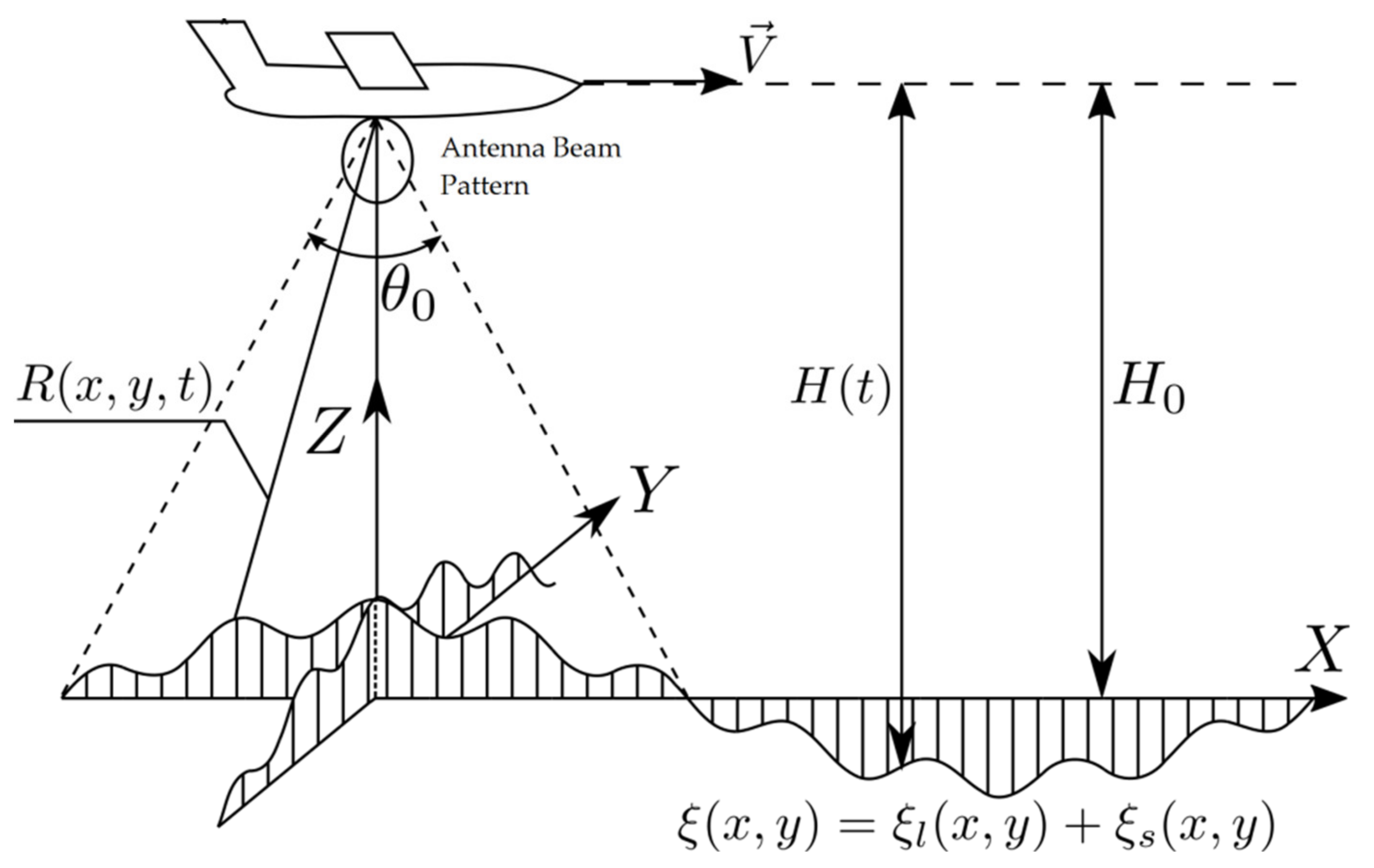
Figure 1.
Vertical profile of a large-scale topography of the sea surface, where H0 is the distance from PRA to the average calm sea surface level, H(t) is the height over sea surface which is time-varying and depends on the slope of large-scale roughness, ξ(t) is the approximation of the large roughness of the sea surface, R(x, y, t) is the slant range from PRA to the sea surface, θ0 is the PRA antenna pattern beamwidth, V is the vehicle velocity. Flying at low altitudes, the radar altimeter provides real-time estimation of the sea wave heights [15].
2. Effect of Local Backscattering Pattern of the Sea Surface on Reflected Signal of PRA at Low Altitudes
The surface is defined as a superposition of large and small roughness that model large wind waves (or swell waves) and small wind waves (or ripples) on the large wave surface:
To find the expression for the voltage at the input of the discriminator, we assume that the number of small irregularities within the irradiated surface is large, and the two-dimensional law of distribution of small irregularities is normal with variance .
Then the final expressions for the voltage values at the input of the discriminator [15]:
where A is the scale factor, G(s,t) is the PRA antenna pattern, R0 is the distance to the average level of the surface, , is the autocorrelation function of the probing signal, ds is the elementary site on the surface, t is the time, c is the speed of light, Glbp is the local backscattering pattern, which is defined by expression
ls is the spatial correlation interval of the small irregularities, is an effective width of the main lobe of the local backscattering pattern, which is determined by the statistical characteristics of small irregularities.
Figure 2 shows the dependence of the local backscattering pattern on time and the surface profile for different widths of the backscattering pattern. The local backscattering pattern is not only a function of sea surface reflective properties but also a function of time. It depends on the relative position of the flying vehicle from the sea surface, as well as on the presence of small ripples on the sea surface [15].
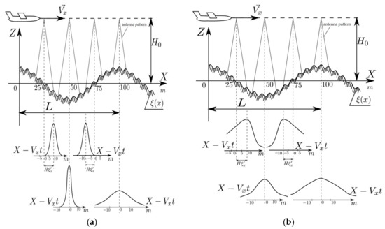
Figure 2.
The dependence of the LBP on time and the profile of the sea surface for different widths of the backscattering pattern Δθlbp at H = 100 m, Vx = 200 m/s, ξ0 = 2 m, L = 100 m, ξ(x) = ξ0 cos(2πx/L): (a) Δθlbp = 0.1 rad; (b) Δθlbp = 0.34 rad.
3. Formulation of the Height Estimate in a Precision Radar Altimeter
Using (2), we find an expression of the discriminator tracking system for height estimation:
where is ambiguity function of square of the envelope of the autocorrelation function of the LFM signal and the reference pulse at frequency shift; is the current detuning of the height estimation in the discriminator, is the distance between the reference signals.
Thus, the discriminator characteristic of PRA, which depends on time and slope of the surface, changes randomly during the flight. At the tracking point we can equalize (4) to zero and obtain the integral equation
With the integral method of signal processing (“centroid”), when reference pulses are much wider than the reflected signals and the mutual uncertainty function slowly changes from , the following approximation is used
Taking into account (6), we transform the integral Equation (5) to the following form:
where is a height estimation.
Solving (7) with respect to , we obtain
Expression (8) defines the algorithm of formulating a height estimation expression with signal integration processing. Due to that the integrands depend on random functions describing large roughness and their slopes, direct calculation of (8) in the general case is impossible.
To analyze the expression of PRA, we consider a special case. Let the derivative of large roughness be constant within the illumination spot. We use antenna pattern approximation to calculate (8):
Substituting (9) into (8) and considering that the following expression is obtained:
In (10) is the bias of the estimate of the height, time-varying, depending on the slopes of major roughness
where is the effective beam width taking into account antenna pattern and local backscattering pattern, and is the component of the height estimation related to surface topography
where .
From (10) height estimation at the output of the tracking system of the PRA is the sum of three factors: the first is the height to the average level; the second is the bias of the estimate of the height, time-varying, depending on the slopes of major roughness; the third is the component related to surface topography.
4. Description of the Sea Surface Roughness
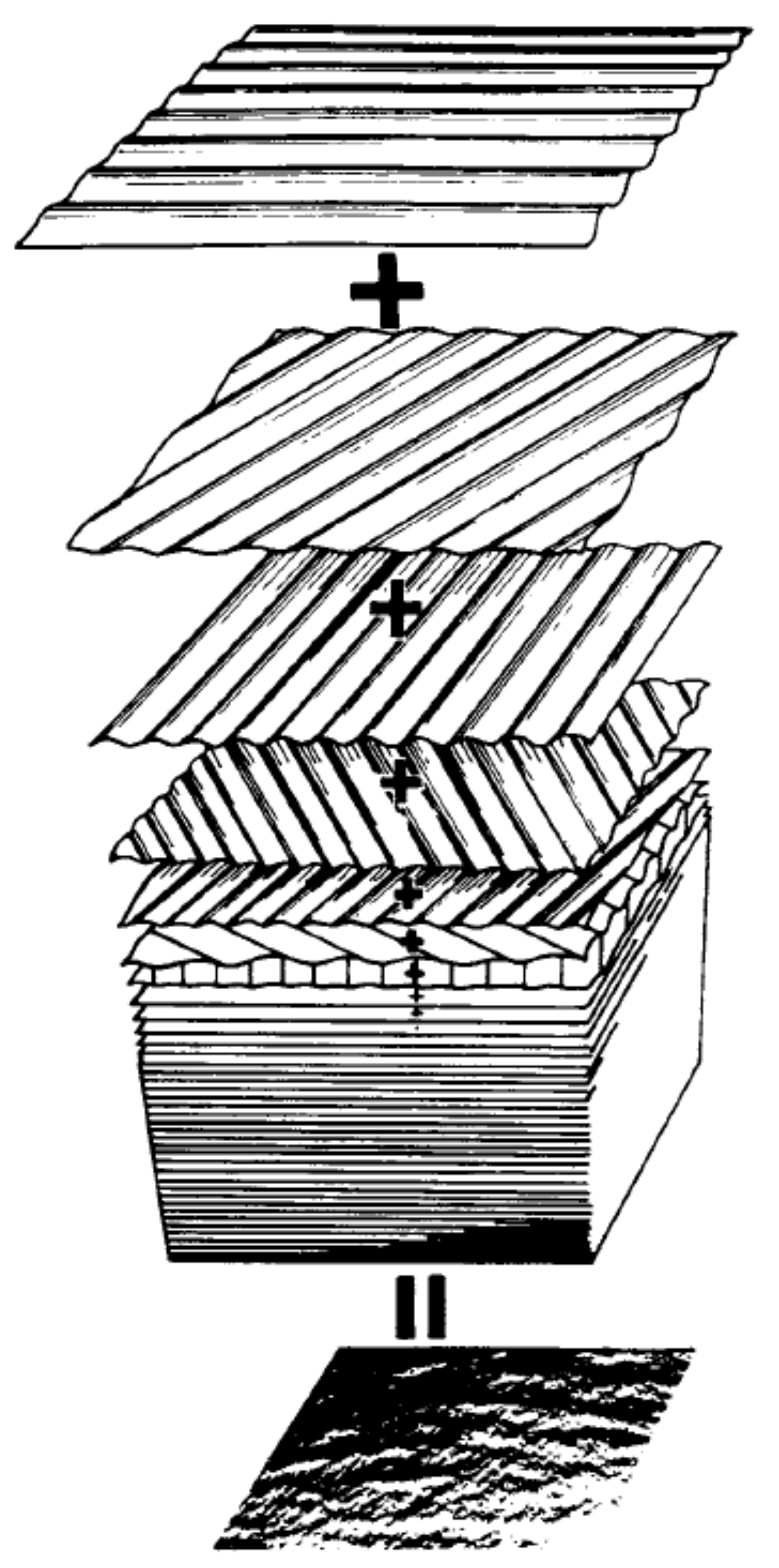
The problem of describing the sea surface roughness can be solved using the principle of superposition (Figure 3), the overlay of simple harmonic waves. Such a superposition underlies the spectral method for sea wave research.

Figure 3.
An illustration of the principle of superposition of sea waves harmonics.
The task of describing an irregular sea surface is solved using the superposition principle represented as the sum of large number of elementary waves [16,17]:
where the sea surface, in this case, is subject to the laws of statistics. It is assumed that the rough sea surface with fully developed waves is locally uniform, stationary, subject to the normal distribution law and has the property of ergodicity. The function S(ω,θ) is a spectral function of two-dimensional energy spectrum.
Among many approximation expressions for the spectra of sea waves, there is a widely used group of so-called exponential spectra. Often used “Joint North Sea Wave Project” (JONSWAP) where the spectrum has the following form [18,19]:
where
The parameter γ is usually 3.3, but for more accurate mathematical calculations the value can be calculated depending on the significant wave height Hm and the repetition period of sea waves Tp:
and lies in the range from 1 to 7.
Frequency spectrum specifies the fluctuations of the sea surface at a fixed point and, therefore, cannot give any information about the distribution of elementary waves energy depending on their direction of propagation. Therefore, frequency-angular spectrum of waves , where function S(ω) describes the distribution of wave energy in frequencies, and the function Q(ω,θ) is responsible for angular distribution, is commonly used.
The cos2l θ function is usually taken as a mathematical model of angular spectrum . It is easy to use, although it has not been confirmed experimentally. Sometimes its extended version is used [20]:
where , The exponent l depends on the wind strength and frequency but known approximations of these dependences differ significantly. For spectrum of wind waves l = 1~4, and for swell l = 6.
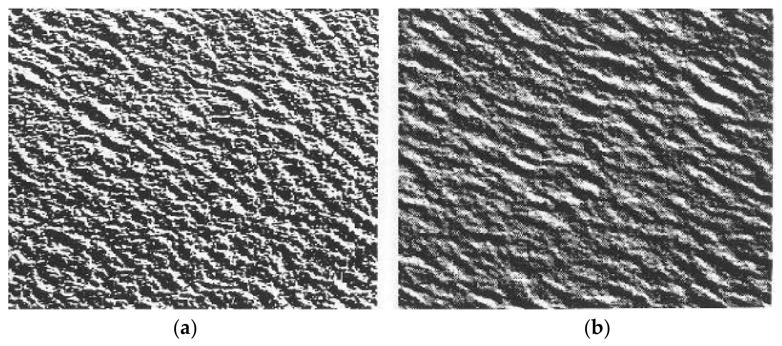
The JONSWAP spectrum has proven itself well for describing developed wind waves, however, it describes only large-scale waves, therefore, the high-frequency part is worked out much worse than the low-frequency one (Figure 4). The real process of wave formation includes, in addition to wind waves, waves of various nature, among which there are swell waves as well. In other words, the formation of waves on the sea surface depends on a very large number of factors, some of which we may not even know yet.

Figure 4.
(a) Photo of the sea surface at the Norwegian coast, (b) the result of sea wave simulation using JONSWAP spectra and angular spectrum cos2lθ [21].
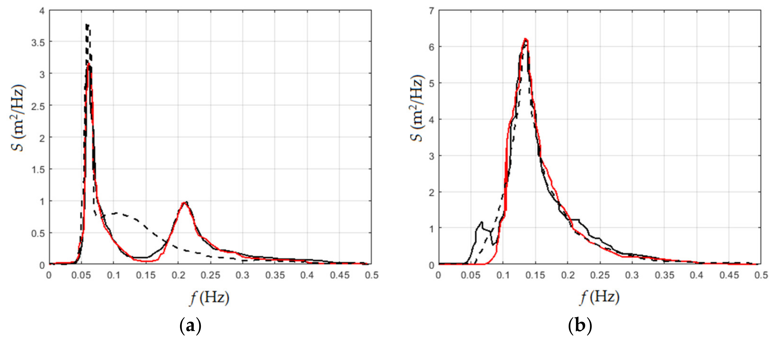
In modern science, the calculation of the sea surface is performed using a two-humped spectrum of sea waves. The imposition of swell waves on the wind component generates two “humps” in the form of sea wave spectrum, as shown in Figure 5.
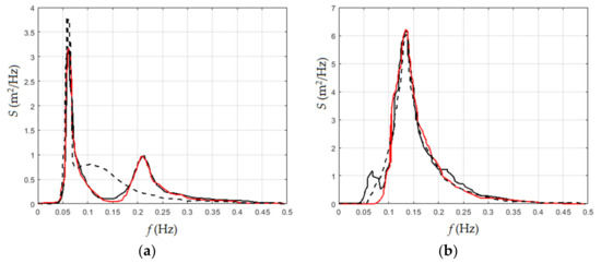
Figure 5.
Various types of double-humped spectra: (a) it is with swell dominance on the left and (b) with wind-driven waves on the right.
The general structure of the spectrum has the form
where is a function that describes the shape of a “hump” in the form of a JONSWAP spectrum.
In accordance with the spectral model selected, the approximation of the sea surface will be written as:
where θp is the angle of the wind propagation direction.
5. Calculation of Limiting Accuracy of Height Measurement in Sea Wave Spectrum Domain
For the calculation of the estimation error, i.e., limiting accuracy of PRA height measurement of a flying vehicle at low over the sea surface, we need reasonable approximations for the large-scale roughness of the sea surface with a deterministic function . In this research, we used the spectral representation of the sea surface instead of a harmonic function approach.
To numerically implement the estimation of the PRA altitude, the operations of differentiation and integration of the expression for the approximation of the sea surface should be performed at x = y = 0. Then the x derivative of the selected sea surface approximation ξx(t) has the following form:
And for y:
The integral included in the (12) is also required to calculate.
As a result, we have the following expression for the height estimation
True altitude of the flying vehicle is determined from the expression
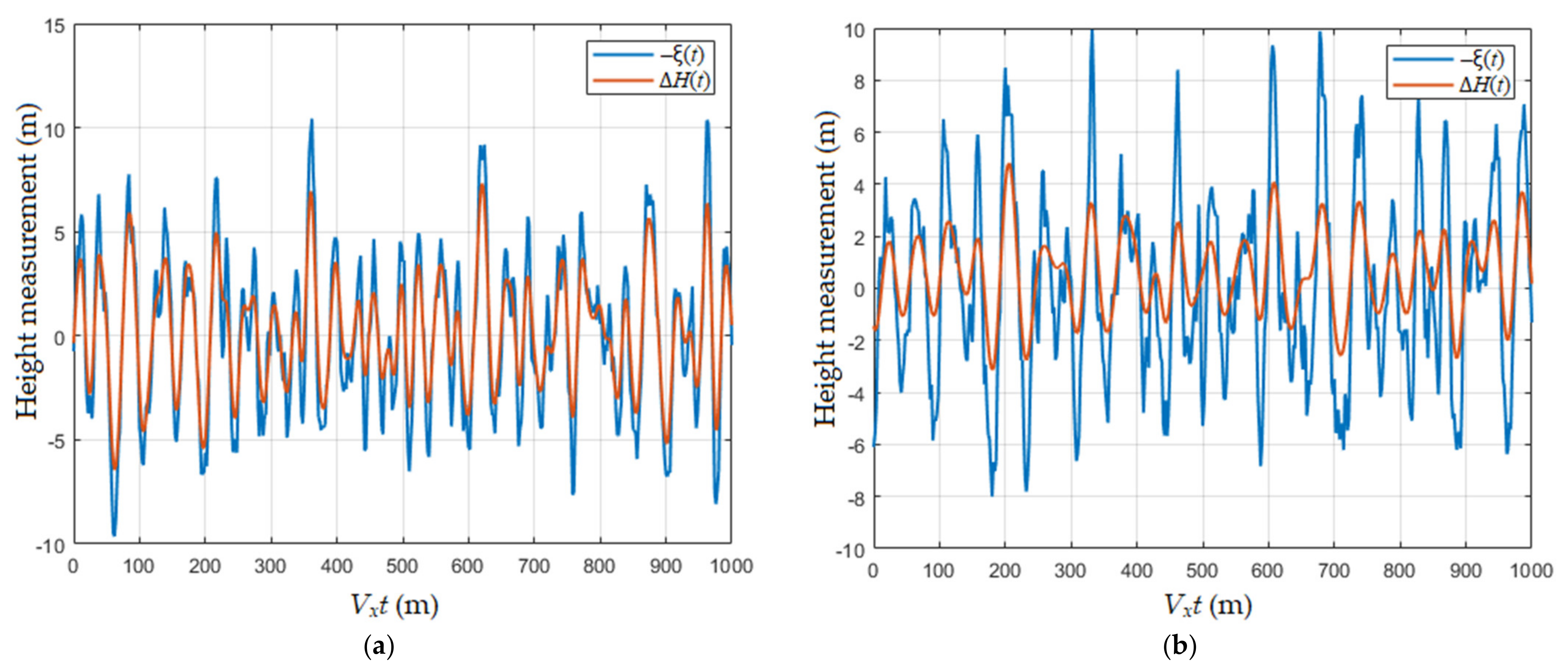
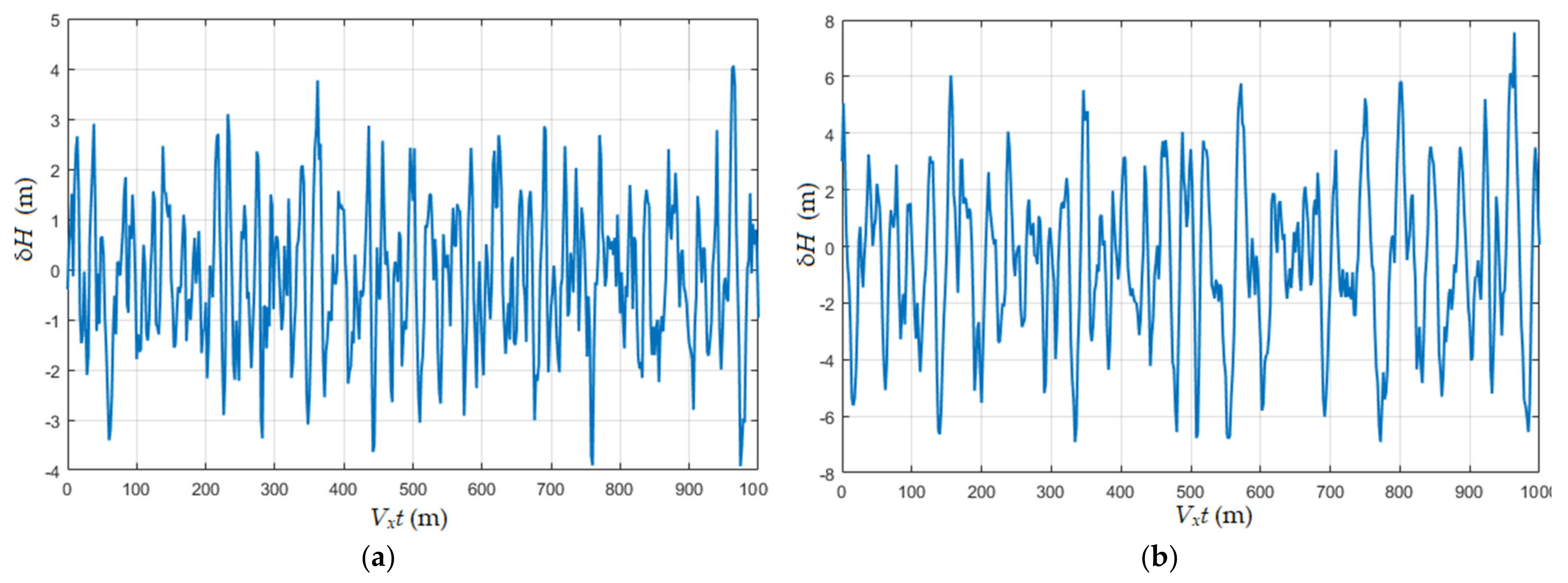
Comparing H(t) and H*(t), we could derive results for the limiting accuracy of the PRA operating at low altitudes above the sea surface, as shown in Figure 6 and Figure 7, where Uw is wind speed, ΔH(t) = H*(t) − H0 and , limiting accuracy.
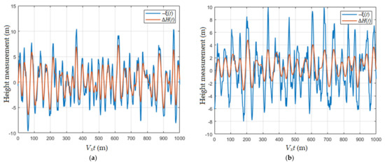
Figure 6.
Increment of the estimation ΔH(t) due to the relief with respect to the sea surface profile (with a minus sign) for Vx = 200 m/s, Vy = 0 m/s, Uw = 20 m/s, θ0 = 0.3 rad: (a) H0 = 50 m; (b) H0 = 100 m.
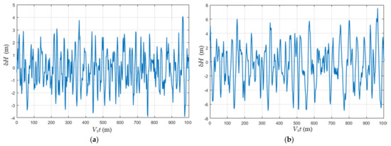
Figure 7.
Limiting accuracy of height measurement for Vx = 200 m/s, Vy = 0 m/s, Uw = 20 m/s, θ0 = 0.3 rad: (a) H0 = 50 m; (b) H0 = 100 m.
6. Conclusions
When the PRA flying at low altitudes during its surface profile measurement, the reflective property of the sea surface is expressed as a function of , which also depends on time and relative position of the flying vehicle to the sea surface in contract to the well-known concepts of backscattering pattern; and its effective beam width is determined by the statistical characteristics of small-scale roughness on the surface of large wind waves; and the location of the maximum of the local backscattering pattern is determined by the derivative of the large-scale roughness of the sea surface, and when the backscattering pattern is wide, the symmetry of the local backscattering pattern on the slopes of the topography is not maintained; all of which are obtained and concluded in our previous research [15].
The direct calculation of the height estimate of the PRA altitude during its signal processing stage is difficult since the integrands in (8) are determined by the random functions which describe large-scale roughness of the sea surface and their slopes.
The height estimation at the output of the tracking system of the PRA is the sum of three factors: the first is the height to the average sea level; the second is the bias from the height, which is time-varying and depends on the slopes of large-scale roughness; the third is the component related to the sea surface topography.
For a quantitative calculation of the estimation error of the height measurement of a flying PRA at low altitudes, a reasonable approximation for the large-scale roughness of the sea surface by the deterministic function is required.
Two-humped frequency spectrum and angular spectrum of the form cos2l θ are used for the approximation of the large-scale roughness.
Analysis of the results shows that as the width of the antenna beam pattern increases by means of flight altitude increasing, the width of the local backscattering pattern and the sea illumination area are increased, which lead to the increase of the estimation error. In this scenario, the systematic error tends to grow unlimitedly, and the random component tends to be constant equal to the standard deviation of the wave height, i.e., the PRA smooths the sea surface roughness.
The approximation developed in this study does not consider small-scale roughness associated with the surface viscosity of the liquid on the sea surface of large wind waves. Therefore, the values of the narrow local backscattering pattern from small-scale roughness in this case were set artificially. Since the inclusion of ripples on waves was not fully covered in this study, it will make sense to consider this issue separately in future works.
The results obtained from this study for the analysis of limiting accuracy of a PRA in a flying vehicle at low altitude above the sea surface, allows to obtain reasonable system parameter values, which minimize the measurement errors of the flight altitude.
Author Contributions
Conceptualization A.I.B. and M.-H.K.; Formal analysis: A.I.B. and A.A.K.; Methodology A.I.B. and A.V.R.; Software A.A.K. and A.V.R.; Supervision A.I.B., A.A.K. and M.-H.K.; Writing A.I.B. and M.-H.K.; Funding A.I.B., A.A.K. and M.-H.K. All authors have read and agreed to the published version of the manuscript.
Funding
This work was financially supported by: RFBR and MCESSM, according to the research project No. 19-57-44001; Basic Science Research Program through the National Research Foundation of Korea (NRF) funded by the Ministry of Education (2021R1A2C2006025), Korea.
Conflicts of Interest
The authors declare no conflict of interest.
References
- Fu, L.-L.; Cazenane, A. Satellite Altimetry and Earth Sciences: A Handbook of Techniques and Applications; Academic: San Diego, CA, USA, 2001. [Google Scholar]
- Zhukovsky, A.P.; Onoprienko, E.I.; Chizhov, V.I. Theoretical Fundamentals of Radio Altimetry; Soviet Radio: Moscow, Russia, 1979. (In Russian) [Google Scholar]
- Baskakov, A.I.; Dzutyaeva, T.S.; Lukashenko, U.I. Radar Remote Sensing of Objects and Environments Research; Akademia Publishing Centre: Moscow, Russia, 2011. (In Russian) [Google Scholar]
- Berger, T. Satellite altimetry using ocean backscatter. IRE Trans. Antennas Propag. 1972, 20, 295–309. [Google Scholar] [CrossRef]
- Baskakov, A.I.; Gagarin, S.P.; Kalinkevitch, A.A.; Kutuza, B.G.; Terekhov, V.A. Simultaneous radiometric and radar altimetric measurements of sea microwave signatures. IEEE J. Ocean. Eng. 1984, 9, 325–328. [Google Scholar] [CrossRef]
- Rodríguez-Morales, F.; Li, J.; Leuschen, C.; Hvidegaard, S.M.; Forsberg, R. Airborne Altimetry Measurements in the Arctic Using a Compact Multi-Band Radar System: Initial Results. In Proceedings of the IGARSS 2020—2020 IEEE International Geoscience and Remote Sensing Symposium, Waikoloa, HI, USA, 26 September–2 October 2020; pp. 3019–3022. [Google Scholar] [CrossRef]
- Halimi, A.; Mailhes, C.; Tourneret, J.; Thibaut, P.; Boy, F. A Semi-Analytical Model for Delay/Doppler Altimetry and Its Estimation Algorithm. IEEE Trans. Geosci. Remote Sens. 2013, 52, 4248–4258. [Google Scholar] [CrossRef] [Green Version]
- Richard, J.; Phalippou, L.; Robert, F.; Stenou, N.; Thouvenot, E.; Sengenes, P. An advanced concept of radar altimetry over oceans with improved performances and ocean sampling: AltiKa. In Proceedings of the 2007 IEEE International Geoscience and Remote Sensing Symposium, Barcelona, Spain, 23–28 July 2007; pp. 3537–3540. [Google Scholar] [CrossRef]
- Egido, A.; Smith, W.H.F. Fully Focused SAR Altimetry: Theory and Applications. IEEE Trans. Geosci. Remote Sens. 2016, 55, 392–406. [Google Scholar] [CrossRef]
- Christophe, F.; Frederic, F.; Eric, M.; Pierre-Louis, F.; Gayane, F.; Pierre, B.; Lionel, J. Spaceborne altimetry and scatterometry backscattering coefficients at C- and Ku-band over West Africa. In Proceedings of the 2014 IEEE Geoscience and Remote Sensing Symposium, Quebec City, QC, Canada, 13–18 July 2014; pp. 3327–3330. [Google Scholar] [CrossRef]
- Dong, X.; Zhang, Y.; Zhai, W.; Shi, X. Spaceborne Interferometric Imaging Radar Altimeter Simulator for Measurement of Global Oceanic Topography. In Proceedings of the 2019 International Radar Conference (RADAR), Toulon, France, 23–27 September 2019; pp. 1–5. [Google Scholar] [CrossRef]
- Min-Ho, H.; Ka, A.; Baskakov, I.; Kononov, A.A. Autocorrelation function of return waveforms in high precision spaceborne radar altimeters employing chip transmit pulse. IEICE Trans. Commun. 2007, 90, 3237–3245. [Google Scholar]
- Baskakov, A.I. The study of the possibility of using signals with linear frequency modulation to assess the excitement of the sea surface. News of higher educational institutions. Radiophysics 1978, XXI, 710–713. (In Russian) [Google Scholar]
- Garnakeryan, A.A.; Sosunov, A.S. Sea Surface Radar; Rostov University: Rostov-on-Don, Russia, 1978. (In Russian) [Google Scholar]
- Ka, M.; Baskakov, A.I.; Artemenko, A. Effect of the local backscattering pattern of the sea surface to the reflected signal of a precision airborne radar altimeter at low altitude. IEEE Geosci. Remote Sens. Lett. 2016, 13, 1246–1249. [Google Scholar] [CrossRef]
- Abuzyarov, Z.K. Sea Surface and Its Forecasting; Gidrometeoizdat: Moscow, Russia, 1981. (In Russian) [Google Scholar]
- Naderi, M.; Pätzold, M. Design and analysis of a one-dimensional sea surface simulator using the sum-of-sinusoids principle. In Proceedings of the OCEANS 2015—MTS/IEEE Washington, Washington, DC, USA, 19–22 October 2015; pp. 1–7. [Google Scholar] [CrossRef]
- Shpektorov, A.G.; Ha, M.T. Modeling the forces and moments of sea waves. Izv. SPbGETU LETI 2013, 2, 43–48. (In Russian) [Google Scholar]
- Mao, Y.; Guo, L.; Ding, H. Numerical simulation for the sea echo spectrum of OTHR radar based on JONSWAP sea spectrum. In Proceedings of the 2011 IEEE International Conference on Microwave Technology & Computational Electromagnetics, Beijing, China, 22–25 May 2011; pp. 369–371. [Google Scholar] [CrossRef]
- Goda, Y. Random Seas and Design of Maritime Structures; University of Tokyo Press: Tokyo, Japan, 1985. [Google Scholar]
- Danièle, H.; Kimmo, K.; Krogstad, H.E.; Susanne, L.; Monbaliu, J.A.J.; Wy-att, L.R. Measuring and Analysing the Directional Spectra of Ocean Waves; Office for Official Publications of the Europeaan Communities: Luxembourg, 2005. [Google Scholar]

Publisher’s Note: MDPI stays neutral with regard to jurisdictional claims in published maps and institutional affiliations. |
© 2021 by the authors. Licensee MDPI, Basel, Switzerland. This article is an open access article distributed under the terms and conditions of the Creative Commons Attribution (CC BY) license (https://creativecommons.org/licenses/by/4.0/).